Bacteria–bacteriophage cycles facilitate Cholera outbreak cycles: an indirect Susceptible-Infected-Recovered-Bacteria- Phage (iSIRBP) model-based mathematical study

Abstract

Cholera is an acute enteric infectious disease caused by the Gram-negative bacterium Vibrio cholerae. Despite a huge body of research, the precise nature of its transmission dynamics has yet to be fully elucidated. Mathematical models can be useful to better understand how an infectious agent can spread and be properly controlled. We develop a compartmental model describing a human population, a bacterial population as well as a phage population. We show that there might be eight equilibrium points, one of which is a disease free equilibrium point. We carry out numerical simulations and sensitivity analyses and we show that the presence of phage can reduce the number of infectious individuals. Moreover, we discuss the main implications in terms of public health management and control strategies.

Keywords:

• Cholera
• bacteriophage
• phage
• basic reproduction number

1. Introduction

Cholera is an acute enteric infectious disease caused by the Gram-negative bacterium Vibrio cholerae (V. cholerae), which spreads by water or food contaminated with feces. It causes diarrhea, which can lead to dehydration that might lead to death within hours if it untreated [7]. Its effect is more dangerous among individuals who have insufficient access to safe water and proper sanitation; it is also more dramatic in areas where basic environmental infrastructures are disrupted or have been destroyed. The World Health Organization (WHO) estimated that there are from 1.3 to 4 million cholera cases and 21,000 to 143,000 deaths due to cholera yearly [19]. However, in countries with adequate health care, cholera imposes a much less dramatic burden.

The precise nature of the cholera transmission dynamics is not clear yet, despite a huge body of research and the many efforts of the scientific community. For example, [4] discussed the response of men to infection with V. cholerae. In [17], Snow's communication model of cholera was proposed. [9] discussed the role of blue-green algae in maintaining endemicity and seasonality of cholera in Bangladesh. [6] proposed that a viable but non-culturable V. cholerae O1 strain can revert to a cultivable state in the human intestine [6], and in [8], the authors discussed a critical element in the ability of V. cholerae to cause outbreaks and epidemics.

It is of paramount importance to understand how V. cholerae can transmit through men. This would enable researchers and public health authorities to monitor the evolution of the outbreak and help put into effect adequate intervention measures that limit the effects of cholera spreading.

Mathematical models of infection transmission dynamics are extremely useful in better understanding how an infectious agent can spread and how can be effectively managed and controlled. More specifically, mathematical modelling of cholera has a long history; through the decades, many models have been devised and proposed. However, few of them have incorporated indirect transmission of the disease. Among these, the major models that employ ordinary differential equations are those built upon improved and branched off versions of the Cappasso and Paveri–Fontana model [3] and the Codeco model [5]. For example, these models include those proposed by [8,10–12,14,18].

The model employed in this project is an extension of the work by [12], which considers the role of the bacteriophage, host and pathogen on the infection's sustainability. The bacteria population is assumed to be divided into two subgroups: non-pathogenic and pathogenic strains. This assumption is due to the fact that the pili protein is produced only by pathogenic strains and is necessary to anchor the bacteria to the wall of the gastrointestinal tract, so that infection can develop. It is during this crucial process that the phage targets the pili protein. The pili and toxin genes are activated by the same bacterial switch, so that toxin is produced during bacterial colonization of the gastrointestinal tract. Noting that only virulent strains of V. cholerae can produce toxin, this biological process is insured thanks to the phage and the bacterium transfer CTX (a genetic sequence that produces the toxin) through a very specific mechanism, see [1].

In the present paper, we find and discuss eight potentially equilibria, one of which is a free equilibrium point. We discuss the major epidemiological properties of the model, perform mathematical simulations and carry out sensitivity analysis to test the robustness of our proposed model.

2. Model formulation

Our model describes the cholera transmission taking into account host, pathogen and bacteriophage dynamics. Here, the phage population is divided into two groups: non-pathogenic and pathogenic strains. In the compartmental model presented, the host population follows a Susceptible-Infectious-Recovered (SIR) framework with S + I + R = N, where N is the total population size, which is kept constant. The bacteria population is described by the compartments and , while P represents the bacteriophage population. Observe that the interaction between bacteria and bacteriophage follows the well-known predator-prey relationship. Hence, we use Holling 1 predation term , where θ is a constant of proportionality, is the conversion rate from non-pathogenic strain to pathogenic strain, induced by phage. is the half saturation constant of predation (the bacteria level at which predation occurs at half the maximum rate). The populations' dynamics is represented by the following system of ordinary differential equations: (1) defines the incidence term, where is the pathogenic bacteria density-dependent component. The indirect part of the incident term is defined as Human contamination of the water supply through infected feces contributes to both bacteria and phage levels and is called shedding and it depends on both bacteria shedding of the infected individuals (a biological quantity) and the level of sanitation in the environment (an environmental assessment). Bacteria and phage shedding rates may not be the same, so the rate for the bacteria is ξ and that for the phage is , where ϕ is constant. The list of model parameters values and their description are seen in Table 1. The ranges of the parameters values were obtained from [4] and [10].

Table 1. Model parameter values, their description and associated units.

Parameter	Description	Values	Unit
r	Maximum per capita pathogen growth efficiency	0.3−14.3
K	Pathogen carrying capacity		Cell
H	Half-saturation pathogen density		Cell
a	Maximum rate of infection	0.1
ξ	Pathogen shed rate	0−100
μ	Human recovery rate	0.1
N	Total population		Persons
c	MID
β	Phage burst size	80−100	Virions
	Maximum per capita phage absorption rate	0-0.025	Cell
	Maximum per capita phage absorption rate	0-0.025	Cell
d	Phage death rate	0.5-7.9
ϕ	Mean phage shed rate		Virions
	Half saturation bacteria predation density		Cell

3. Forward invariance

We would like to identify a forwardly invariant set in which solutions of system (1(1) ) will be bounded.

From the first equation of system (1(1) ), we see that . Thus for t>0. From the second equation of system (1(1) ), we see that if I = 0, then . Since by definition, and for t>0, we get that . If R = 0, then form the third equation of system (1(1) ), we get , and hence . As S + I + R = N, we must have .

Clearly, if P = 0, then , and hence .

If , then from Equation (6) of system (1(1) ) we get that , thus . Similarly, if , then from Equation (4) we have , and hence .

To find an upper bound for , let . Then Set . Now, If B = 0, then . Moreover, has two real roots, namely and Clearly, .

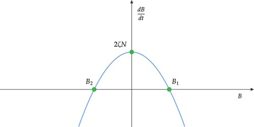
The graph of is shown in Figure 1. Since , we conclude that . Thus is bounded above.

Figure 1. The graph of .

Since , and both are non-negative, we get .

Finally, to find an upper bound for , the following lemma is needed.

Lemma 3.1

Define positive constants such that . Then for all values of B, the following is true:

To show that is bounded above, let . Then Let . Then .

Now, by solving the ordinary differential equation , we get that for some constant c. Consequently, we get We summarize the previous results is in the following proposition:

Proposition 3.2

Let . Then the set defines a forward invariant region of system (1(1) ), where and .

4. Equilibria with no shedding and their stability

In this section, we determine the equilibrium points of the model system when , and then perform stability analysis of the equilibria. Since is a non-smooth function, to ease our analysis, we study the dynamics of the system when separately.

4.1. Existence of equilibria

Substituting in system (1(1) ) and noticing that R = N−S−I, the third equation is then not necessary. Thus system (1(1) ) reduces to (2) To analyse the types of solutions that this model could produce, a steady-state analysis was performed. The algebraic analysis is provided in the Supplementary Material.

Case 1: If the pathogenic bacteria level is below or equal to the minimum infectious dose, then . Hence system (2(2) ) becomes (3) Then system (3(3) ) has four disease-free equilibrium points which are listed below:

1. always exists.

2. always exists, where m is a non-negative constant such that if , then , and if K>c, then .

   Special cases of are:

   1. .

   2. where .

3. exists if . In this case, is such that if , then , and if K>c, then , so that .

4. The interior point exits if the following conditions hold:

   1. .

   2. . Note that the existence of and is contrary.

   3. .

   4. .

   5. .

Case 2: If the pathogenic bacteria level is above the minimum infectious dose, then , leaving us with the following system: (4) Let . Then, one can easily check that if , and hence if

. Consequently, Solving the last three equations of system (4(4) ), we get the following equilibrium points:

1. exists if K>c.

   In this case, m is a positive constant such that if K>c, then .

   Special case of is where K>c.

2. exists if .

   In this case, is such , so that

   .

3. The interior point exits if the following conditions are hold:

   1. .

   2. . Note that the existence of and is contrary.

   3. .

   4. .

   5. .

4.2. Stability of equilibria

Depending on the pathogenic bacteria level, the linearization of system (2(2) ) has two forms, one for system (3(3) ) when , denoted by J, and one for system (4(4) ) when , denoted by .

The stability of the equilibria are stated in Theorem 4.1 and that of the equilibria are stated in Theorem 4.2.

Let Then, we have

Theorem 4.1

The equilibrium point is always unstable. The equilibrium point might be stable if , and consequently the equilibrium point might be stable if and the equilibrium point might be stable if . That is, might be unstable if exists. The equilibrium point if exists, is always unstable.

Proof.

Set: and . Then the Jacobian matrix for model system (3(3) ) is given as follows:

Let be the Jacobian matrix evaluated at , .

From the Jacobian matrix , it is found that its eigenvalues are and r. Since r>0, then is always unstable.

From the Jacobian matrix , it is found that its eigenvalues are and . Hence, might be stable if the following condition holds: Considering the special case , we get the following eigenvalues: . Thus if , then might be stable, and if , then might be unstable.

When considering the equilibrium point , we found that the eigenvalues corresponding to are: and . So, might be stable if , which is equivalent to say that might be stable if . But if exists, then and hence, might be unstable whenever exists.

From the Jacobian matrix , it is found that none of the eigenvalues is zero, and one of the eigenvalue is . Now, if , then But in order for to be positive, we must have . Thus we conclude that , and hence is unstable whenever it exists.

Theorem 4.2

The equilibrium point might be stable if where the equilibrium point might be stable if . The equilibrium point if exists, is always unstable.

Proof.

Set: and . Then the Jacobian matrix for model system (4(4) ) is given as follows:

Let be the Jacobian matrix evaluated at , .

From the Jacobian matrix , it is found that the eigenvalues are: and . Hence, might be stable if .

Considering the equilibrium point , we get the following eigenvalues: and . Hence, might be stable if

From the Jacobian matrix , it is found that none of the eigenvalues is zero and one of the eigenvalues is , which was shown in the proof of Theorem (4.1) to be positive. Thus , if exists, is unstable.

5. Equilibria with shedding and their stability

In this section, we determine the equilibrium points of the model system when , and then perform stability analysis of the equilibria.

5.1. Existence of equilibria

Noting that as R = N−S−I the third equation of system (1(1) ) is not necessary, leaving us with the following system: (5) If , then we will have the same equilibrium points and as in Section 4.1, with the same conditions.

If , then , and hence at steady state system (5(5) ) reduces to (6) Then system (6(6) ) has one equilibrium point, namely which exists if the following condition holds: where , and , with . , where The proof of the existence of is provided in the Supplementary Material.

5.2. Stability of equilibria

For the equilibrium points we lack exact expressions for the equilibrium quantities, and so the local stability is difficult to be found analytically.

6. Sensitivity analysis

The objective of this section is to discuss the sensitivity of the peak value and time to model parameters. The ranges of the parameters values were obtained from [4] and [10]. We assume that recovered patient immediately become susceptible. We equally assume that within the period of our studies, deaths and births are equal. Thus our system reduces to the following system: (7) Using the normalized forward sensitivity index, we study the sensitivity of the parameters of System (7(7) ) to cholera outbreak peak and peak time. The normalized forward sensitivity index: (8) where is the quantity being considered (peak value or peak time) and p is a parameter which depends upon. Sensitivity indices can be positive or negative which indicates the nature of the relationship, and it is the magnitude that ranks the strength of the relationship as compared to the other parameters. Because we do not have an explicit formula for the quantities we are interested in (outbreak peak, outbreak peak time and the endemic steady state), we estimate using the central difference approximation: We choose of p. plugging all these in (8(8) ) we get Figure 2 contains the sensitivity of the outbreak peak and the outbreak peak time to the parameters of the model.

Figure 2. The sensitivity of the magnitude of outbreak peak and peak time to the parameters: (a) the sensitivity of the outbreak peak to the parameters while (b) the sensitivity of the outbreak peak time to the parameters.

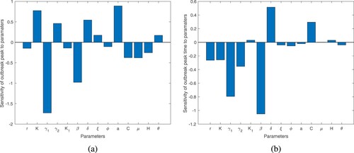
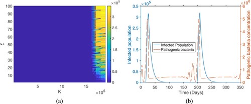
Figure 3 shows reservoir related parameters: phage attack rate and phage burst size have the strongest relationships to the magnitude of the outbreak peak and outbreak peak time. The figure shows that if the phage attack rate and burst sizes are large, the magnitude of the outbreak peak value will be small and the time at which it occurs will be large. This indicates that phage-bacteria predator prey like cycles may have a key role to play in driving cholera outbreak cycles. Looking at the two parameters that can be controlled by policy-makers, these are K and ξ. The carrying capacity K has a large influence on the dynamics of the system. It has one of the largest sensitivity indices, being many times greater than that of the shedding rate ξ. Figure a shows the sensitivity indices of the outbreak to these two important parameters. The figure shows that the outbreak peak value increase as K but almost has no response to the variation in ξ. This further emphasizes the importance of paying attention to the dynamics in the reservoir in order to control and prevent outbreaks. The figure shows that if there are good sanitation practices that prevent shedding, but without taking care of the dynamics in the reservoir the bacteria-phage dynamics may still be able to cause outbreak in human population. This is clearly illustrated in the figure. In Figure b we plot the time course dynamics of infected population (left y-axis) and pathogenic bacteria population (right y-axis). The parameter values are chosen in such a way that we have two outbreaks every year. In such a situation, the figure illustrates that the bacteria population peaks before the human population. This indicates that the bacteria–bacteriophage cycles in the reservoir may be driving the outbreak cycles in the human population.

Figure 3. Microscopic cycles in the reservoir drives the macroscopic cycles in human population. (a) Sensitivity of the out break peak to K and ξ. K varies from 100 to and ξ varies from 1 to 100. (b) Time course dynamics of the infected population and pathogenic phage level in the reservoir.

Our finding that the bacteria–bacteriophage cycles in the reservoir may be driving the outbreak cycles in the human population has important practical implications in terms of public health policies. Our model confirms and expands empirical and theoretical proofs that lytic bacteriophages are one of the major drivers of cholera infection, shedding light on the complex interplay between the host, pathogen and phages [15]. Cholera is one of the infectious diseases for which ecological factors and indirect transmission routes play a major role, together with those infections caused by pathogens like rotavirus, hantavirus, Legionella, Schistosoma, Cryptosporidium or Giardia. Devising mathematical models which incorporate bacteriophages can shed light on the epidemiological features of cholera and provide a better understanding of it. The seasonal self-limiting pattern of cholera epidemics can be explained taking into account the phage predation behaviour of the V. cholerae during the late stages of the outbreak, which are usually characterized by significant phage shedding in stools. Bacteriophages are able to tune/modulate the bacterial infectivity and, as such, to lead to the collapse/quenching of the outbreak, with a very low probability of a phage-resistant variant to take-over [16]. Advancements in the understanding of phages/bacteria interactions could potentially lead to the development of tools for monitoring and even predicting (forecasting/now-casting) of cholera outbreaks. For instance, it has been suggested that phage monitoring in acquatic environments and reservoirs could be a feasible strategy for controlling and mitigating against the burden imposed by cholera [16]. Moreover, recent discoveries have shown that cocktails based on a number of virulent bacteriophages can effectively prevent V. cholerae infection [20]. Phage therapy appears to be a promising pharmacological tool to counteract cholera transmission, given the organizational difficulties to implement mass vaccination campaigns in low-resource contexts as well as the lack of drugs and the issue imposed by multi-drug resistance [2,13]. In conclusion, mathematical models could play a significant role in elucidating the mechanisms of such a therapy, helping physicians optimize it [10]. As such, further research is warranted.

7. Conclusion

Cholera is an acute enteric infectious disease which imposes a relevant societal and clinical burden in developing countries, characterized by inadequate access to water, sanitation and lacking of proper healthcare facilities. Despite a huge body of research, the precise nature of cholera transmission dynamics has yet to be fully elucidated. Mathematical models can be useful to better understand how an infectious agent can spread and be properly controlled. In the present paper, we developed a compartmental model describing a human population, a bacterial population as well as a phage population. We showed that there might be up to eight equilibrium points; one of which is a disease free equilibrium point. We carried out numerical simulations and sensitivity analyses and we showed that the presence of phages can significantly reduce the number of infectious individuals. Moreover, we discussed the main implications in terms of public health management and control strategies. Our results agree with empirical and theoretical proofs that lytic bacteriophages are one of the major drivers of cholera infection [15]. Our findings support [16]'s suggestion that phage monitoring in acquatic environments and reservoirs could be a feasible strategy for controlling and mitigating cholera outbreaks. Moreover, our results suggest that phages could be used to efficiently treat V. cholerae infections. This is in line with the findings in [2,10,13,20]. Our proposed model can inform public health policies in low-resource settings, helping health policy- and decision-makers implement evidence-informed programs aimed at targeting cholera outbreaks and epidemics. Moreover, our model can be further expanded and refined, inspiring further research in the field.

Disclosure statement

No potential conflict of interest was reported by the author(s).

Additional information

Funding

J.D.K. acknowledges support from Canada's International Development Research Centre (IDRC) (Grant No. 109559-001). The main idea of this paper came from a conversation JDK had with Hao Wang and Edwin Pos.

References

- Bacteriophage makes Vibrio Cholerae deadly, Lab Med. 28(1) (1997), pp. 8–9.
- S. Bhandare, J. Colom, A. Baig, J.M. Ritchie, H. Bukhari, M.A. Shah, B.L. Sarkar, J. Su, B. Wren, P. Barrow, and R.J. Atterbury, Reviving phage therapy for the treatment of cholera, J. Infect. Dis. 219(5) (2019), pp. 786–794.
- V. Capasso and S.L. Paveri-Fontana, A mathematical model for the 1973 cholera epidemic in the European Mediterranean region, Rev. Epidemiol. Sante. Publique. 27(2) (1979), pp. 121–132.
- R.A. Cash, S.I. Music, J.P. Libonati, M.J. Snyder, R.P. Wenzel, and R.B. Hornick, Response of man to infection with Vibrio cholerae. I. Clinical, serologic, and bacteriologic responses to a known inoculum, J. Infect. Dis. 129(1) (1974), pp. 45–52.
- C.T. Codeo, Endemic and epidemic dynamics of cholera: the role of the aquatic reservoir, BMC Infect. Dis. 1(1) (2001), pp. 1–14.
- R.R. Colwell, P. Brayton, D. Herrington, B. Tall, A. Huq, and M.M. Levine, Viable but non-culturable Vibrio cholerae O1 revert to a cultivable state in the human intestine, World J. Microbiol. Biotechnol. 12(1) (1996), pp. 28–31.
- R.A. Finkelstein, Cholera, Vibrio cholerae O1 and O139, and other pathogenic vibrios 4th ed., Medical Microbiology, 1996.
- D.M. Hartley, J.G. Morris Jr, and D.L. Smith, Hyperinfectivity: a critical element in the ability of V. cholerae to cause epidemics? PLoS Med. 3(1) (2006), pp. e7.
- M.S. Islam, B.S. Drasar, and R.B. Sack, Probable role of blue-green algae in maintaining endemicity and seasonality of cholera in Bangladesh: A hypothesis, J. Diarrhoeal. Dis. Res. 12(4) (1994), pp. 245–256.
- M.A. Jensen, S.M. Faruque, J.J. Mekalanos, and B.R. Levin, Modeling the role of bacteriophage in the control of cholera outbreaks, PNAS 103(12) (2006), pp. 4652–4657.
- R. I. Joh, H. Wang, H. Weiss, and J. S. Weitz, Dynamics of indirectly transmitted infectious diseases with immunological threshold, Bull. Math. Biol. 71(4) (2009), pp. 845–862.
- J.D. Kong, W. Davis, and H. Wang, Dynamics of a cholera transmission model with immunological threshold and natural phage control in reservoir, Bull. Math. 76(8) (2014), pp. 2025–2051.
- J.F. Miller, Bacteriophage and the evolution of epidemic cholera, Infect. Immun. 71(6) (2003), pp. 2981–2982.
- Z. Mukandavire, S. Liao, J. Wang, H. Gaff, D.L. Smith, and J.G. Morris, Estimating the reproductive numbers for the 2008–2009 cholera outbreaks in Zimbabwe, PNAS 108(21) (2011), pp.8767–8772.
- E.J. Nelson, J.B. Harris, J.G. Morris, S.B. Calderwood, and A. Camilli, Cholera transmission: the host, pathogen and bacteriophage dynamic, Nat. Rev. Microbiol. 7(10) (2009), pp. 693–702.
- C.A. Silva-Valenzuela and A. Camilli, Niche adaptation limits bacteriophage predation of Vibrio cholerae in a nutrient-poor aquatic environment, PNAS 116(5) (2019), pp. 1627–1632.
- J. Snow, On the Mode of Communication of Cholera, John Churchill, London, 1855.
- J.P. Tian and J. Wang, Global stability for cholera epidemic models, Math. Biosci. 232(1) (2011), pp. 31–41.
- World Health Organization, Cholera. Available at https://www.who.int/news-room/fact-sheets/detail/cholera.
- M. Yen, L.S. Cairns, and A. Camilli, A cocktail of three virulent bacteriophages prevents Vibrio cholerae infection in animal models, Nat. Commun. 8(1) (2017), pp. 1–7.