Hopf bifurcation in delayed nutrient-microorganism model with network structure

Abstract

In this paper, we introduce and deal with the delayed nutrient-microorganism model with a random network structure. By employing time delay τ as the main critical value of the Hopf bifurcation, we investigate the direction of the Hopf bifurcation of such a random network nutrient-microorganism model. Noticing that the results of the direction of the Hopf bifurcation in a random network model are rare, we thus try to use the method of multiple time scales (MTS) to derive amplitude equation and determine the direction of the Hopf bifurcation. It is showed that the delayed random network nutrient-microorganism model can exhibit a supercritical or subcritical Hopf bifurcation. Numerical experiments are performed to verify the validity of the theoretical analysis.

Keywords:

• Nutrient-microorganism model
• Hopf bifurcation
• amplitude equation
• random network

1. Introduction

The existence of the Hopf bifurcation in ecological systems is a hot investigation field, since its practical significance in biological control. Therefore, there are many results concerning the Hopf bifurcation in ecological systems that have been reported, see Refs. [5–7,12]. One of the most important results induced by the Hopf bifurcation is periodic solutions, including spatially homogeneous and spatially non-homogeneous periodic solutions. As a result, it is necessary to study or determine the stability of the periodic solution. As we know, there are two common techniques to study the direction of the Hopf bifurcation in a delayed differential equation, they are centre manifold reduction (CMR) and MTS, see Refs. [2,8,11].

It is noticed that there are few results about the direction of the Hopf bifurcation in a delayed reaction-diffusion system with network structure have been reported [9,10], where the direction of the Hopf bifurcation is determined by employing the method of CMR. However, different from the technique is adopted in [9,10], we mainly attempt to use MTS to compute amplitude equation, and determine the direction of the Hopf bifurcation in a delayed nutrient-microorganism model with random network structure. More precisely, the system we consider takes the form (1) $\begin{array}{r}\{\begin{array}{l}{\displaystyle \frac{\mathrm{d}{u}_i}{\mathrm{d}t}=d_1\sum _{j=1}^N{\mathrm{\Delta }}_{ij}{u}_i+\beta u_i(\frac{u_i{v}_i}{u_i+K}-1),}\\ {\displaystyle \frac{\mathrm{d}{v}_i}{\mathrm{d}t}=d_2\sum _{j=1}^N{\mathrm{\Delta }}_{ij}{v}_i+\alpha -v_i(t-\tau )-\frac{u_i^2{v}_i}{u_i+K},}\\ {\displaystyle u_i(0)>0,v_i(0)>0.}\end{array}\end{array}$(1) This model is called nutrient-microorganism system in the sediment, and first proposed by Baurmann and Feudel in [1](continuous form). All parameters $d_1,d_2,\alpha ,\beta ,K$ in (1(1) $\begin{array}{r}\{\begin{array}{l}{\displaystyle \frac{\mathrm{d}{u}_i}{\mathrm{d}t}=d_1\sum _{j=1}^N{\mathrm{\Delta }}_{ij}{u}_i+\beta u_i(\frac{u_i{v}_i}{u_i+K}-1),}\\ {\displaystyle \frac{\mathrm{d}{v}_i}{\mathrm{d}t}=d_2\sum _{j=1}^N{\mathrm{\Delta }}_{ij}{v}_i+\alpha -v_i(t-\tau )-\frac{u_i^2{v}_i}{u_i+K},}\\ {\displaystyle u_i(0)>0,v_i(0)>0.}\end{array}\end{array}$(1) ) are positive constants; $\tau \ge 0$ is time delay, it implies that some time delay is required for microorganism to consume nutrient in the sediment.

For system (1(1) $\begin{array}{r}\{\begin{array}{l}{\displaystyle \frac{\mathrm{d}{u}_i}{\mathrm{d}t}=d_1\sum _{j=1}^N{\mathrm{\Delta }}_{ij}{u}_i+\beta u_i(\frac{u_i{v}_i}{u_i+K}-1),}\\ {\displaystyle \frac{\mathrm{d}{v}_i}{\mathrm{d}t}=d_2\sum _{j=1}^N{\mathrm{\Delta }}_{ij}{v}_i+\alpha -v_i(t-\tau )-\frac{u_i^2{v}_i}{u_i+K},}\\ {\displaystyle u_i(0)>0,v_i(0)>0.}\end{array}\end{array}$(1) ), we assume that it is defined on an undirected network with N nodes and there are no self-loops; $u_i$ and $v_i$ are the densities of the microorganism and the nutrient on node i, respectively; $\mathbf{\Delta }$ is the $N\times N$ discrete Laplacian matrix of network with its elements ${\mathrm{\Delta }}_{ij}=k_i{\delta }_{ij}-L_{ij}$, where $\mathbf{L}$ is the adjacency matrix encoding the network connection, this indicates it satisfies $L_{ij}=1$ if there is a link connecting from patch i to patch j. If not, $L_{ij}=0$ when there is no any link connecting from patch i to patch j, and ${\delta }_{ij}$ is the Kronecker's delta [4]. Moreover, the degree of the ith node is defined by $k_i=\sum _{j=1}^N{L}_{ij}$, and the connection probability between node i and node j for $i\ne j$ is $p(0\le p\le 1)$.

This paper is structured as follows. In Section 2, we establish the existence results of the Hopf bifurcation of the model (1). In Section 3, the amplitude equation of the Hopf bifurcation is deduced. As a result, the supercritical or the subcritical Hopf bifurcation can be yield by analysing the amplitude equation. We perform the numerical simulations to verify the theoretical analysis in Section 4, and some discussions are made in Section 5.

2. Existence of the Hopf bifurcation

In this section, we give some conditions to ensure the existence of the Hopf bifurcation of the networked model (1). To this end, we first consider the existence and stability of positive equilibria for model (1).

Lemma 2.1

[3]

The possible positive equilibria of model (1) can be found as follows

(i)	if $\alpha <1+2\sqrt{K}$, model (1) has no positive equilibrium;
(ii)	if $\alpha >1+2\sqrt{K}$, model (1) has two positive equilibria $E_1^{\ast }=(u_1^{\ast },v_1^{\ast })$ and $E_2^{\ast }=(u_2^{\ast },v_2^{\ast })$. Here $v_1^{\ast }=\alpha -u_1^{\ast },v_2^{\ast }=\alpha -u_2^{\ast }$ and $u_1^{\ast }=\frac{1}{2}(\alpha -1+\sqrt{(\alpha -1{)}^2-4K}),u_2^{\ast }=\frac{1}{2}(\alpha -1-\sqrt{(\alpha -1{)}^2-4K}),$
(iii)	if $\alpha =1+2\sqrt{K}$, model (1) has one positive equilibrium $E_3^{\ast }=(u_3^{\ast },v_3^{\ast })=(\sqrt{K},1+\sqrt{K})$.

Lemma 2.2

[3]

When diffusion and delay are absent, the following statements are valid.

(i)	If $\alpha =1+2\sqrt{K}$, the positive equilibrium $E_3^{\ast }$ is unstable when $\beta >2+\frac{1}{\sqrt{K}}$;
(ii)	If $\alpha >1+2\sqrt{K}$, the positive equilibrium $E_2^{\ast }$ is unstable and the positive equilibrium $E_1^{\ast }$ is locally asymptotically stable when $\beta <{\beta }_0^H$ and unstable when $\beta >{\beta }_0^H$, where ${\beta }_0^H=\frac{\alpha u_1^{\ast }}{K}$.

Thereby, in view of Lemma 2.1 and Lemma 2.2, we only focus on the dynamical behaviours near $E_1^{\ast }$, and we denote it by $E_1^{\ast }\triangleq E_{\ast }=(u_{\ast },v_{\ast })$ for simplicity. Now, we shall perform the linear stability analysis of system (1) near the positive equilibrium $E_{\ast }=(u_{\ast },v_{\ast })$. For this purpose, let $\mathrm{\Gamma }{u}_i=u_i-u_{\ast }$ and $\mathrm{\Gamma }{v}_i=v_i-v_{\ast }$ be the small perturbations, then the linear system of (1) evaluated at $E_{\ast }=(u_{\ast },v_{\ast })$ can be written as follows (2) $\begin{array}{r}\left(\begin{array}{c}\mathrm{\Gamma }{\dot{u}}_i\\ \mathrm{\Gamma }{\dot{v}}_i\end{array}\right)=J_1\left(\begin{array}{c}\mathrm{\Gamma }{u}_i\\ \mathrm{\Gamma }{v}_i\end{array}\right)+J_2\left(\begin{array}{c}\mathrm{\Gamma }{u}_{i\tau }\\ \mathrm{\Gamma }{v}_{i\tau }\end{array}\right)+D\left(\begin{array}{c}\sum _{j=1}^N{\mathrm{\Delta }}_{ij}\mathrm{\Gamma }{u}_j\\ \sum _{j=1}^N{\mathrm{\Delta }}_{ij}\mathrm{\Gamma }{v}_j\end{array}\right),\end{array}$(2) where $u_i=u_i(t),u_{i\tau }=u_{i\tau }(t-\tau )$ and $J_1=\left(\begin{array}{cc}{\displaystyle \frac{\beta K}{u_{\ast }+K}}& {\displaystyle \frac{\beta u_{\ast }}{v_{\ast }}}\\ -1-{\displaystyle \frac{K}{u_{\ast }+K}}& -{\displaystyle \frac{u_{\ast }}{v_{\ast }}}\end{array}\right),J_2=\left(\begin{array}{cc}0& 0\\ 0& -1\end{array}\right),D=\left(\begin{array}{cc}{d}_1& 0\\ 0& d_2\end{array}\right).$Let $0={\mathrm{\Lambda }}_1>{\mathrm{\Lambda }}_2>\cdot \cdot \cdot >{\mathrm{\Lambda }}_N$ be the eigenvalues of the discrete Laplacian matrix $\mathbf{\Delta }$, and suppose that ${\mathfrak{L}}_{\varphi }=\{{\varphi }_i{\}}_{i=1}^N$ is the subspace generated by the eigenfunctions associated to the topological eigenvalue ${\mathrm{\Lambda }}_i$. Then, the general solution of system (2) can be rewritten as $\left(\begin{array}{c}\mathrm{\Gamma }{u}_i\\ \mathrm{\Gamma }{v}_i\end{array}\right)=\sum _{i=1}^N\left(\begin{array}{c}{\xi }_1\\ {\xi }_2\end{array}\right){\varphi }_i{e}^{{\lambda }_{i}t},$with $\sum _{j=1}^N{\mathrm{\Delta }}_{ij}{\varphi }_j={\mathrm{\Lambda }}_i{\varphi }_i$. Inserting them into (2), one has $\left(\begin{array}{cc}{\displaystyle \frac{\beta K}{u_{\ast }+K}}+d_1{\mathrm{\Lambda }}_i& {\displaystyle \frac{\beta u_{\ast }}{v_i^{\ast }}}\\ -1-{\displaystyle \frac{K}{u_{\ast }+K}}& -{\displaystyle \frac{u_{\ast }}{v_{\ast }}}-e^{-{\lambda }_i\tau }+d_2{\mathrm{\Lambda }}_i\end{array}\right)\left(\begin{array}{c}{\xi }_1\\ {\xi }_2\end{array}\right)={\lambda }_i\left(\begin{array}{c}{\xi }_1\\ {\xi }_2\end{array}\right).$It then follows that (3) $\begin{array}{r}{\lambda }_i^2+{\mathcal{A}}_{{\mathrm{\Lambda }}_i}{\lambda }_i+({\lambda }_i+{\mathcal{B}}_{{\mathrm{\Lambda }}_i})e^{-{\lambda }_i\tau }+{\mathcal{C}}_{{\mathrm{\Lambda }}_i}=0,\end{array}$(3) where $\begin{array}{rl}& {\mathcal{A}}_{{\mathrm{\Lambda }}_i}=-(d_1+d_2){\mathrm{\Lambda }}_i+\frac{u_{\ast }}{v_{\ast }}-\frac{\beta K}{u_{\ast }+K},\\ & {\mathcal{B}}_{{\mathrm{\Lambda }}_i}=-d_1{\mathrm{\Lambda }}_i-\frac{\beta K}{u_{\ast }+K},\\ & {\mathcal{C}}_{{\mathrm{\Lambda }}_i}=d_1{d}_2{\mathrm{\Lambda }}_i^2-(\frac{u_{\ast }{d}_1}{v_{\ast }}-\frac{d_2\beta K}{u_{\ast }+K}){\mathrm{\Lambda }}_i+\frac{\beta u_{\ast }}{v_{\ast }}.\end{array}$Let $\lambda =i\omega (\omega >0)$ be the solution of Equation (3), we have ${\omega }^4+({\mathcal{A}}_{{\mathrm{\Lambda }}_i}^2-2{\mathcal{C}}_{{\mathrm{\Lambda }}_i}-1){\omega }^2+{\mathcal{C}}_{{\mathrm{\Lambda }}_i}^2-{\mathcal{B}}_{{\mathrm{\Lambda }}_i}^2=0.$Thereby, if one of the conditions in the following $\begin{array}{rl}({\mathcal{H}}_0)& {\mathcal{C}}^2-{\mathcal{B}}^2<0,\\ ({\mathcal{H}}_1)& {\mathcal{C}}^2-{\mathcal{B}}^2=0,{\mathcal{A}}^2-2\mathcal{C}-1<0,\\ ({\mathcal{H}}_2)& {\mathcal{C}}^2-{\mathcal{B}}^2>0,{\mathcal{A}}^2-2\mathcal{C}-1<0,({\mathcal{A}}^2-2\mathcal{C}-1{)}^2-4({\mathcal{C}}^2-{\mathcal{B}}^2)=0,\end{array}$is satisfied, one yields (4) $\begin{array}{r}{\omega }_{{\mathrm{\Lambda }}_i}^2=\frac{1}{2}(1+2{\mathcal{C}}_{{\mathrm{\Lambda }}_i}-{\mathcal{A}}_{{\mathrm{\Lambda }}_i}^2+\sqrt{({\mathcal{A}}_{{\mathrm{\Lambda }}_i}^2-2{\mathcal{C}}_{{\mathrm{\Lambda }}_i}-1{)}^2-4({\mathcal{C}}_{{\mathrm{\Lambda }}_i}^2-{\mathcal{B}}_{{\mathrm{\Lambda }}_i}^2)}).\end{array}$(4) We thus obtain the critical value τ of the Hopf bifurcation is (5) $\begin{array}{r}{\tau }_{{\mathrm{\Lambda }}_i}^j=\{\begin{array}{l}{\displaystyle \frac{1}{{\omega }_{{\mathrm{\Lambda }}_i}}}\arccos \left\{{\displaystyle \frac{({\mathcal{B}}_{{\mathrm{\Lambda }}_i}-{\mathcal{A}}_{{\mathrm{\Lambda }}_i}){\omega }_{{\mathrm{\Lambda }}_i}^2-{\mathcal{B}}_{{\mathrm{\Lambda }}_i}{\mathcal{C}}_{{\mathrm{\Lambda }}_i}}{{\omega }_{{\mathrm{\Lambda }}_i}^2+{\mathcal{B}}_{{\mathrm{\Lambda }}_i}^2}}\right\}+{\displaystyle \frac{2j\pi }{{\omega }_{{\mathrm{\Lambda }}_i}}},\sin {\omega }_{{\mathrm{\Lambda }}_i}{\tau }_{{\mathrm{\Lambda }}_i}^j>0,\\ {\displaystyle \frac{-1}{{\omega }_{{\mathrm{\Lambda }}_i}}}\arccos \left\{{\displaystyle \frac{({\mathcal{B}}_{{\mathrm{\Lambda }}_i}-{\mathcal{A}}_{{\mathrm{\Lambda }}_i}){\omega }_{{\mathrm{\Lambda }}_i}^2-{\mathcal{B}}_{{\mathrm{\Lambda }}_i}{\mathcal{C}}_{{\mathrm{\Lambda }}_i}}{{\omega }_{{\mathrm{\Lambda }}_i}^2+{\mathcal{B}}_{{\mathrm{\Lambda }}_i}^2}}\right\}+{\displaystyle \frac{2(j+1)\pi }{{\omega }_{{\mathrm{\Lambda }}_i}}},\sin {\omega }_{{\mathrm{\Lambda }}_i}{\tau }_{{\mathrm{\Lambda }}_i}^j<0,\end{array}\end{array}$(5) where $j\in {\mathbb{N}}_0=\{0,1,2,\dots \}$. In addition, a straightforward calculation shows that $\begin{array}{rl}\mathbf{R}\mathbf{e}{\left\{{\left(\frac{\text{d}\lambda }{\text{d}\tau }\right)}^{-1}\right\}}_{\tau ={\tau }_{{\mathrm{\Lambda }}_i}^j}& =\mathbf{R}\mathbf{e}{\{\frac{({\mathcal{A}}_{{\mathrm{\Lambda }}_i}+2\lambda )e^{\lambda \tau }+1}{\lambda (\lambda +{\mathcal{B}}_{{\mathrm{\Lambda }}_i})}-\frac{\tau }{\lambda }\}}_{\tau ={\tau }_{{\mathrm{\Lambda }}_i}^j}\\ & =\mathbf{R}\mathbf{e}{\left\{\frac{({\mathcal{A}}_{{\mathrm{\Lambda }}_i}+2\lambda )e^{\lambda \tau }+1}{\lambda (\lambda +{\mathcal{B}}_{{\mathrm{\Lambda }}_i})}\right\}}_{\tau ={\tau }_{{\mathrm{\Lambda }}_i}^j}\\ & =\mathbf{R}\mathbf{e}\left\{\frac{({\mathcal{A}}_{{\mathrm{\Lambda }}_i}+2i{\omega }_{{\mathrm{\Lambda }}_i})(\cos {\omega }_{{\mathrm{\Lambda }}_i}{\tau }_{{\mathrm{\Lambda }}_i}^j+i\sin {\omega }_{{\mathrm{\Lambda }}_i}{\tau }_{{\mathrm{\Lambda }}_i}^j)+1}{i{\omega }_{{\mathrm{\Lambda }}_i}(i{\omega }_{{\mathrm{\Lambda }}_i}+{\mathcal{B}}_{{\mathrm{\Lambda }}_i})}\right\}\\ & =\frac{{\mathcal{A}}_{{\mathrm{\Lambda }}_i}^2-2{\mathcal{C}}_{{\mathrm{\Lambda }}_i}-1+2{\omega }_{{\mathrm{\Lambda }}_i}^2}{{\omega }_{{\mathrm{\Lambda }}_i}^2+{\mathcal{B}}_{{\mathrm{\Lambda }}_i}^2}\\ & =\frac{\sqrt{({\mathcal{A}}_{{\mathrm{\Lambda }}_i}^2-2C_{{\mathrm{\Lambda }}_i}-1{)}^2-4({\mathcal{C}}_{{\mathrm{\Lambda }}_i}^2-{\mathcal{B}}_{{\mathrm{\Lambda }}_i}^2)}}{{\omega }_{{\mathrm{\Lambda }}_i}^2+{\mathcal{B}}_{{\mathrm{\Lambda }}_i}^2}\\ & >0.\end{array}$Moreover, note that $\text{Sign}\left\{\mathbf{R}\mathbf{e}{\left\{{\left(\frac{\text{d}\lambda }{\text{d}\tau }\right)}^{-1}\right\}}_{\tau ={\tau }_{{\mathrm{\Lambda }}_i}^j}\right\}=\text{Sign}\left\{\mathbf{R}\mathbf{e}{\left\{\frac{\text{d}\lambda }{\text{d}\tau }\right\}}_{\tau ={\tau }_{{\mathrm{\Lambda }}_i}^j}\right\},$this implies that the transversality condition of the Hopf bifurcation is satisfied. Combine this with (5(5) $\begin{array}{r}{\tau }_{{\mathrm{\Lambda }}_i}^j=\{\begin{array}{l}{\displaystyle \frac{1}{{\omega }_{{\mathrm{\Lambda }}_i}}}\arccos \left\{{\displaystyle \frac{({\mathcal{B}}_{{\mathrm{\Lambda }}_i}-{\mathcal{A}}_{{\mathrm{\Lambda }}_i}){\omega }_{{\mathrm{\Lambda }}_i}^2-{\mathcal{B}}_{{\mathrm{\Lambda }}_i}{\mathcal{C}}_{{\mathrm{\Lambda }}_i}}{{\omega }_{{\mathrm{\Lambda }}_i}^2+{\mathcal{B}}_{{\mathrm{\Lambda }}_i}^2}}\right\}+{\displaystyle \frac{2j\pi }{{\omega }_{{\mathrm{\Lambda }}_i}}},\sin {\omega }_{{\mathrm{\Lambda }}_i}{\tau }_{{\mathrm{\Lambda }}_i}^j>0,\\ {\displaystyle \frac{-1}{{\omega }_{{\mathrm{\Lambda }}_i}}}\arccos \left\{{\displaystyle \frac{({\mathcal{B}}_{{\mathrm{\Lambda }}_i}-{\mathcal{A}}_{{\mathrm{\Lambda }}_i}){\omega }_{{\mathrm{\Lambda }}_i}^2-{\mathcal{B}}_{{\mathrm{\Lambda }}_i}{\mathcal{C}}_{{\mathrm{\Lambda }}_i}}{{\omega }_{{\mathrm{\Lambda }}_i}^2+{\mathcal{B}}_{{\mathrm{\Lambda }}_i}^2}}\right\}+{\displaystyle \frac{2(j+1)\pi }{{\omega }_{{\mathrm{\Lambda }}_i}}},\sin {\omega }_{{\mathrm{\Lambda }}_i}{\tau }_{{\mathrm{\Lambda }}_i}^j<0,\end{array}\end{array}$(5) ) we claim that the delayed network model (1) undergoes the Hopf bifurcation at $E_{\ast }$ when $\tau ={\tau }_{{\mathrm{\Lambda }}_i}^j$ for $0={\mathrm{\Lambda }}_1>{\mathrm{\Lambda }}_2>\cdot \cdot \cdot >{\mathrm{\Lambda }}_N$ and $j\in {\mathbb{N}}_0$. Especially, the delayed network model (1) admits a Hopf bifurcation at $E_{\ast }$ when $\tau ={\tau }_0^0$, and in this case the periodic solution bifurcated from the Hopf bifurcation is spatially homogeneous.

3. Direction of the Hopf bifurcation

In this section, we shall employ MTS to derive amplitude equations and determine the direction of the Hopf bifurcation. We first define ${\tau }_0^0\triangleq {\tau }_{\ast },{\omega }_0\triangleq {\omega }_{\ast }$ and $\tau \to t/\tau$, where ${\omega }_0$ and ${\tau }_0^0$ can be found in (4(4) $\begin{array}{r}{\omega }_{{\mathrm{\Lambda }}_i}^2=\frac{1}{2}(1+2{\mathcal{C}}_{{\mathrm{\Lambda }}_i}-{\mathcal{A}}_{{\mathrm{\Lambda }}_i}^2+\sqrt{({\mathcal{A}}_{{\mathrm{\Lambda }}_i}^2-2{\mathcal{C}}_{{\mathrm{\Lambda }}_i}-1{)}^2-4({\mathcal{C}}_{{\mathrm{\Lambda }}_i}^2-{\mathcal{B}}_{{\mathrm{\Lambda }}_i}^2)}).\end{array}$(4) ) and (5(5) $\begin{array}{r}{\tau }_{{\mathrm{\Lambda }}_i}^j=\{\begin{array}{l}{\displaystyle \frac{1}{{\omega }_{{\mathrm{\Lambda }}_i}}}\arccos \left\{{\displaystyle \frac{({\mathcal{B}}_{{\mathrm{\Lambda }}_i}-{\mathcal{A}}_{{\mathrm{\Lambda }}_i}){\omega }_{{\mathrm{\Lambda }}_i}^2-{\mathcal{B}}_{{\mathrm{\Lambda }}_i}{\mathcal{C}}_{{\mathrm{\Lambda }}_i}}{{\omega }_{{\mathrm{\Lambda }}_i}^2+{\mathcal{B}}_{{\mathrm{\Lambda }}_i}^2}}\right\}+{\displaystyle \frac{2j\pi }{{\omega }_{{\mathrm{\Lambda }}_i}}},\sin {\omega }_{{\mathrm{\Lambda }}_i}{\tau }_{{\mathrm{\Lambda }}_i}^j>0,\\ {\displaystyle \frac{-1}{{\omega }_{{\mathrm{\Lambda }}_i}}}\arccos \left\{{\displaystyle \frac{({\mathcal{B}}_{{\mathrm{\Lambda }}_i}-{\mathcal{A}}_{{\mathrm{\Lambda }}_i}){\omega }_{{\mathrm{\Lambda }}_i}^2-{\mathcal{B}}_{{\mathrm{\Lambda }}_i}{\mathcal{C}}_{{\mathrm{\Lambda }}_i}}{{\omega }_{{\mathrm{\Lambda }}_i}^2+{\mathcal{B}}_{{\mathrm{\Lambda }}_i}^2}}\right\}+{\displaystyle \frac{2(j+1)\pi }{{\omega }_{{\mathrm{\Lambda }}_i}}},\sin {\omega }_{{\mathrm{\Lambda }}_i}{\tau }_{{\mathrm{\Lambda }}_i}^j<0,\end{array}\end{array}$(5) ), respectively. Now, a rewritten form of the networked system (1) can be read as (6) $\begin{array}{r}{\dot{\mathbf{U}}}_i=\tau {\mathbf{L}}_t{\mathbf{U}}_i+\tau {\mathbf{L}}_{\tau }{\mathbf{U}}_{i\tau }+\tau \mathbf{F}({\mathbf{U}}_i),\end{array}$(6) where we set ${\mathbf{U}}_i=(u_i,v_i{)}^T,{\mathbf{U}}_{i\tau }=(u_{i\tau }(t-1),v_{i\tau }(t-1){)}^T$, and ${\mathbf{L}}_t=\left(\begin{array}{cc}{d}_1\sum _{j=1}^N{\mathrm{\Delta }}_{ij}+a_{11}& a_{12}\\ a_{21}& d_2\sum _{j=1}^N{\mathrm{\Delta }}_{ij}+a_{22}\end{array}\right),{\mathbf{L}}_{\tau }=\left(\begin{array}{cc}0& 0\\ 0& -1\end{array}\right),$with $a_{11}=\frac{\beta K}{u_{\ast }+K},a_{12}=\frac{\beta u_{\ast }}{v_{\ast }},a_{21}=-1-\frac{K}{u_{\ast }+K},a_{22}=-\frac{u_{\ast }}{v_{\ast }}.$In addition, the nonlinear term $\mathbf{F}({\mathbf{U}}_i)=(F^{(1)}(U_i),F^{(2)}(U_i){)}^T$ takes the form $\begin{array}{rl}{F}^{(1)}(U_i)& =f_{u_i{u}_i}{u}_i^2+f_{u_i{v}_i}{u}_i{v}_i+f_{u_i{u}_i{u}_i}{u}_i^3+f_{u_i{u}_i{v}_i}{u}_i^2{v}_i+\mathcal{O}(4),\\ F^{(2)}(U_i)& =g_{u_i{u}_i}{u}_i^2+g_{u_i{v}_i}{u}_i{v}_i+g_{u_i{u}_i{u}_i}{u}_i^3+g_{u_i{u}_i{v}_i}{u}_i^2{v}_i+\mathcal{O}(4),\end{array}$with $\begin{array}{rl}{f}_{u_i{u}_i}& =\frac{\beta v_{\ast }{K}^2}{(u_{\ast }+K{)}^3},f_{u_i{u}_i{u}_i}=-\frac{\beta v_{\ast }{K}^2}{(u_{\ast }+K{)}^4},\\ f_{u_i{u}_i{v}_i}& =\frac{\beta K^2}{(u_{\ast }+K{)}^3},f_{u_i{v}_i}=\frac{\beta u_{\ast }(u_{\ast }+2K)}{(u_{\ast }+K{)}^2},\\ g_{u_i{u}_i{u}_i}& =\frac{v_{\ast }{K}^2}{(u_{\ast }+K{)}^4},g_{u_i{u}_i}=-\frac{v_{\ast }{K}^2}{(u_{\ast }+K{)}^3},\\ g_{u_i{u}_i{v}_i}& =-\frac{K^2}{(u_{\ast }+K{)}^3},g_{u_i{v}_i}=-\frac{u_{\ast }(u_{\ast }+2K)}{(u_{\ast }+K{)}^2}.\end{array}$To employ the technique of MTS, let ε be a small perturbation parameter. Then introducing the time scales $T_0=t,T_2={\epsilon }^{2}t$, this induces that (7) $\begin{array}{r}\frac{\mathrm{\partial }}{\mathrm{\partial }t}=\frac{\mathrm{\partial }}{\mathrm{\partial }{T}_0}+{\epsilon }^2\frac{\mathrm{\partial }}{\mathrm{\partial }{T}_2}.\end{array}$(7) Solution ${\mathbf{U}}_i$ can be decribed as (8) $\begin{array}{rl}{\mathbf{U}}_i(T_0,T_2)=\left(\begin{array}{c}{u}_i(T_0,T_2)\\ v_i(T_0,T_2)\end{array}\right)& =\epsilon \left(\begin{array}{c}{u}_i^{(1)}(T_0,T_2)\\ v_i^{(1)}(T_0,T_2)\end{array}\right)+{\epsilon }^2\left(\begin{array}{c}{u}_i^{(2)}(T_0,T_2)\\ v_i^{(2)}(T_0,T_2)\end{array}\right)\\ & +{\epsilon }^3\left(\begin{array}{c}{u}_i^{(3)}(T_0,T_2)\\ v_i^{(3)}(T_0,T_2)\end{array}\right)+\mathcal{O}(4).\end{array}$(8) We thus obtain a fact that (9) $\begin{array}{rl}{U}_{i\tau }(T_0-1,T_2)=\left(\begin{array}{c}{u}_{i\tau }(T_0-1,T_2)\\ v_{i\tau }(T_0-1,T_2)\end{array}\right)& =\sum _{j=1}^3{\epsilon }^j\left(\begin{array}{c}{u}_{i\tau }^{(j)}(T_0-1,T_2)\\ v_{i\tau }^{(j)}(T_0-1,T_2)\end{array}\right)\\ & -{\epsilon }^3\frac{\mathrm{\partial }}{\mathrm{\partial }{T}_2}\left(\begin{array}{c}{u}_{i\tau }^{(1)}(T_0-1,T_2)\\ v_{i\tau }^{(1)}(T_0-1,T_2)\end{array}\right)+\cdots .\end{array}$(9) By a similar manner, we can write the nonlinear term $\mathbf{F}$ as follows (10) $\begin{array}{r}\mathbf{F}={\epsilon }^2{\mathbf{F}}^{(2)}+{\epsilon }^3{\mathbf{F}}^{(3)}+\mathcal{O}({\epsilon }^4),\end{array}$(10) where ${\mathbf{F}}^{(2)}=\left(\begin{array}{c}{f}_{u_i{u}_i}{\left(u_i^{(1)}\right)}^2+f_{u_i{v}_i}{u}_i^{(1)}{v}_i^{(1)}\\ g_{u_i{u}_i}{\left(u_i^{(1)}\right)}^2+g_{u_i{v}_i}{u}_i^{(1)}{v}_i^{(1)}\end{array}\right),$and $F^{(3)}=\left(\begin{array}{c}2f_{u_i{u}_i}{u}_i^{(1)}{u}_i^{(2)}+f_{u_i{v}_i}(u_i^{(1)}{v}_i^{(2)}+u_i^{(2)}{v}_i^{(1)})\\ +f_{u_i{u}_i{u}_i}{\left(u_i^{(1)}\right)}^3+f_{u_i{u}_i{v}_i}{\left(u_i^{(1)}\right)}^2{v}_i^{(1)}\\ 2g_{u_i{u}_i}{u}_i^{(1)}{u}_i^{(2)}+g_{u_i{v}_i}(u_i^{(1)}{v}_i^{(2)}+u_i^{(2)}{v}_i^{(1)})\\ +g_{u_i{u}_i{u}_i}{\left(u_i^{(1)}\right)}^3+g_{u_i{u}_i{v}_i}{\left(u_i^{(1)}\right)}^2{v}_i^{(1)}\end{array}\right),$Next, we introduce the small perturbation of the Hopf bifurcation parameter $\tau ={\tau }_{\ast }+{\epsilon }^2\delta$ with $\delta >0$. Keep this in mind, denote ${\mathbf{L}}_t{|}_{\tau ={\tau }_{\ast }}={\mathbf{L}}_t^{\ast },{\mathbf{L}}_{\tau }{|}_{\tau ={\tau }_{\ast }}={\mathbf{L}}_{\tau }^{\ast }$ and put (7)-(10) into (6), one has

$\mathcal{O}(\epsilon )$: (11) $\begin{array}{r}\frac{\mathrm{\partial }}{\mathrm{\partial }{T}_0}\left(\begin{array}{c}{u}_i^{(1)}\\ v_i^{(1)}\end{array}\right)-{\tau }_{\ast }{\mathbf{L}}_t^{\ast }\left(\begin{array}{c}{u}_i^{(1)}\\ v_i^{(1)}\end{array}\right)-{\tau }_{\ast }{\mathbf{L}}_{\tau }^{\ast }\left(\begin{array}{c}{u}_{i\tau }^{(1)}\\ v_{i\tau }^{(1)}\end{array}\right)=\mathbf{0}.\end{array}$(11) $\mathcal{O}({\epsilon }^2)$: (12) $\begin{array}{r}\frac{\mathrm{\partial }}{\mathrm{\partial }{T}_0}\left(\begin{array}{c}{u}_i^{(2)}\\ v_i^{(2)}\end{array}\right)-{\tau }_{\ast }{\mathbf{L}}_t^{\ast }\left(\begin{array}{c}{u}_i^{(2)}\\ v_i^{(2)}\end{array}\right)-{\tau }_{\ast }{\mathbf{L}}_{\tau }^{\ast }\left(\begin{array}{c}{u}_{i\tau }^{(2)}\\ v_{i\tau }^{(2)}\end{array}\right)={\tau }_{\ast }{\mathbf{F}}^{(2)}.\end{array}$(12) $\mathcal{O}({\epsilon }^3)$: (13) $\begin{array}{rl}& \frac{\mathrm{\partial }}{\mathrm{\partial }{T}_0}\left(\begin{array}{c}{u}_i^{(3)}\\ v_i^{(3)}\end{array}\right)-{\tau }_{\ast }{\mathbf{L}}_t^{\ast }\left(\begin{array}{c}{u}_i^{(3)}\\ v_i^{(3)}\end{array}\right)-{\tau }_{\ast }{\mathbf{L}}_{\tau }^{\ast }\left(\begin{array}{c}{u}_{i\tau }^{(3)}\\ v_{i\tau }^{(3)}\end{array}\right)\\ & =-\frac{\mathrm{\partial }}{\mathrm{\partial }{T}_2}\left(\begin{array}{c}{u}_i^{(1)}\\ v_i^{(1)}\end{array}\right)-{\tau }_{\ast }{\mathbf{L}}_{\tau }^{\ast }\frac{\mathrm{\partial }}{\mathrm{\partial }{T}_2}\left(\begin{array}{c}{u}_{i\tau }^{(1)}\\ v_{i\tau }^{(1)}\end{array}\right)+\delta {\mathbf{L}}_t^{\ast }\left(\begin{array}{c}{u}_i^{(1)}\\ v_i^{(1)}\end{array}\right)\\ & +\delta {\mathbf{L}}_{\tau }^{\ast }\left(\begin{array}{c}{u}_{i\tau }^{(1)}\\ v_{i\tau }^{(1)}\end{array}\right)+{\tau }_{\ast }{\mathbf{F}}^{(3)}.\end{array}$(13) Considering the solution of perturbation Equation (11(11) $\begin{array}{r}\frac{\mathrm{\partial }}{\mathrm{\partial }{T}_0}\left(\begin{array}{c}{u}_i^{(1)}\\ v_i^{(1)}\end{array}\right)-{\tau }_{\ast }{\mathbf{L}}_t^{\ast }\left(\begin{array}{c}{u}_i^{(1)}\\ v_i^{(1)}\end{array}\right)-{\tau }_{\ast }{\mathbf{L}}_{\tau }^{\ast }\left(\begin{array}{c}{u}_{i\tau }^{(1)}\\ v_{i\tau }^{(1)}\end{array}\right)=\mathbf{0}.\end{array}$(11) ) near the Hopf mode, we have (14) $\begin{array}{r}\left(\begin{array}{c}{u}_i^{(1)}\\ v_i^{(1)}\end{array}\right)=H(T_2)\mathbf{p}{e}^{i{\omega }_{\ast }{\tau }_{\ast }{T}_0}+\overline{H}(T_2)\overline{\mathbf{p}}{e}^{-i{\omega }_{\ast }{\tau }_{\ast }{T}_0},\end{array}$(14) where we assume that $H(T_2)$ is the complex amplitude and $\mathbf{p}=\left(\begin{array}{c}1\\ {\displaystyle \frac{i{\omega }_{\ast }-a_{11}}{a_{12}}}\end{array}\right)\triangleq \left(\begin{array}{c}{p}_{11}\\ p_{12}\end{array}\right).$We thus obtain $\begin{array}{rl}& {\left(u_i^{(1)}\right)}^2=H^2(T_2)e^{2i{\omega }_{\ast }{\tau }_{\ast }{T}_0}+2|H(T_2){|}^2+{\overline{H}}^2(T_2)e^{-2i{\omega }_{\ast }{\tau }_{\ast }{T}_0},\\ & u_i^{(1)}{v}_i^{(1)}=p_{12}{H}^2(T_2)e^{2i{\omega }_{\ast }{\tau }_{\ast }{T}_0}+2Re\{p_{12}\}|H(T_2){|}^2+{\overline{p}}_{12}{\overline{H}}^2(T_2)e^{-2i{\omega }_{\ast }{\tau }_{\ast }{T}_0}.\end{array}$This means that the perturbation Equation (12(12) $\begin{array}{r}\frac{\mathrm{\partial }}{\mathrm{\partial }{T}_0}\left(\begin{array}{c}{u}_i^{(2)}\\ v_i^{(2)}\end{array}\right)-{\tau }_{\ast }{\mathbf{L}}_t^{\ast }\left(\begin{array}{c}{u}_i^{(2)}\\ v_i^{(2)}\end{array}\right)-{\tau }_{\ast }{\mathbf{L}}_{\tau }^{\ast }\left(\begin{array}{c}{u}_{i\tau }^{(2)}\\ v_{i\tau }^{(2)}\end{array}\right)={\tau }_{\ast }{\mathbf{F}}^{(2)}.\end{array}$(12) ) has a particular solution with the form (15) $\begin{array}{rl}\left(\begin{array}{c}{u}_i^{(2)}\\ v_i^{(2)}\end{array}\right)& =H^2(T_2)\left(\begin{array}{c}{q}_{11}\\ q_{12}\end{array}\right)e^{2i{\omega }_{\ast }{\tau }_{\ast }{T}_0}+\left(\begin{array}{c}{q}_{21}\\ q_{22}\end{array}\right)|H(T_2){|}^2\\ & +{\overline{H}}^2(T_2)\left(\begin{array}{c}{\overline{q}}_{11}\\ {\overline{q}}_{12}\end{array}\right)e^{-2i{\omega }_{\ast }{\tau }_{\ast }{T}_0},\end{array}$(15) where the vectors $(q_{11},q_{12}{)}^T$ and $(q_{21},q_{22}{)}^T$ are unknown. Thence, to determine them we should insert (15(15) $\begin{array}{rl}\left(\begin{array}{c}{u}_i^{(2)}\\ v_i^{(2)}\end{array}\right)& =H^2(T_2)\left(\begin{array}{c}{q}_{11}\\ q_{12}\end{array}\right)e^{2i{\omega }_{\ast }{\tau }_{\ast }{T}_0}+\left(\begin{array}{c}{q}_{21}\\ q_{22}\end{array}\right)|H(T_2){|}^2\\ & +{\overline{H}}^2(T_2)\left(\begin{array}{c}{\overline{q}}_{11}\\ {\overline{q}}_{12}\end{array}\right)e^{-2i{\omega }_{\ast }{\tau }_{\ast }{T}_0},\end{array}$(15) ) into (12(12) $\begin{array}{r}\frac{\mathrm{\partial }}{\mathrm{\partial }{T}_0}\left(\begin{array}{c}{u}_i^{(2)}\\ v_i^{(2)}\end{array}\right)-{\tau }_{\ast }{\mathbf{L}}_t^{\ast }\left(\begin{array}{c}{u}_i^{(2)}\\ v_i^{(2)}\end{array}\right)-{\tau }_{\ast }{\mathbf{L}}_{\tau }^{\ast }\left(\begin{array}{c}{u}_{i\tau }^{(2)}\\ v_{i\tau }^{(2)}\end{array}\right)={\tau }_{\ast }{\mathbf{F}}^{(2)}.\end{array}$(12) ). Then equating like terms of $e^{2i{\omega }_{\ast }{\tau }_{\ast }{T}_0}{H}^2(T_2)$ and $|H(T_2){|}^2$, we have $\begin{array}{rl}{q}_{11}& =\frac{a_{12}(g_{u_i{u}_i}+p_{12}{g}_{u_i{v}_i})+(2i{\omega }_{\ast }-a_{22}+e^{-2i{\omega }_{\ast }{\tau }_{\ast }})(f_{u_i{u}_i}+p_{12}{f}_{u_i{v}_i})}{(2i{\omega }_{\ast }-a_{11})(2i{\omega }_{\ast }-a_{22}+e^{-2i{\omega }_{\ast }{\tau }_{\ast }})-a_{12}{a}_{21}},\\ q_{12}& =\frac{(2i{\omega }_{\ast }-a_{11})q_{11}-(f_{u_i{u}_i}+p_{12}{f}_{u_i{v}_i})}{a_{12}},\\ q_{21}& =\frac{2a_{12}(g_{u_i{u}_i}+\mathbf{R}\mathbf{e}\{p_{12}\}{g}_{u_i{v}_i})-2(a_{22}-1)(f_{u_i{u}_i}+\mathbf{R}\mathbf{e}\{p_{12}\}{f}_{u_i{v}_i})}{a_{11}(a_{22}-1)-a_{12}{a}_{21}},\\ q_{22}& =-\frac{a_{11}{q}_{21}+2(f_{u_i{u}_i}+\mathbf{R}\mathbf{e}\{p_{12}\}{f}_{u_i{v}_i})}{a_{12}}.\end{array}$As a result, it follows from (14(14) $\begin{array}{r}\left(\begin{array}{c}{u}_i^{(1)}\\ v_i^{(1)}\end{array}\right)=H(T_2)\mathbf{p}{e}^{i{\omega }_{\ast }{\tau }_{\ast }{T}_0}+\overline{H}(T_2)\overline{\mathbf{p}}{e}^{-i{\omega }_{\ast }{\tau }_{\ast }{T}_0},\end{array}$(14) ) and (15(15) $\begin{array}{rl}\left(\begin{array}{c}{u}_i^{(2)}\\ v_i^{(2)}\end{array}\right)& =H^2(T_2)\left(\begin{array}{c}{q}_{11}\\ q_{12}\end{array}\right)e^{2i{\omega }_{\ast }{\tau }_{\ast }{T}_0}+\left(\begin{array}{c}{q}_{21}\\ q_{22}\end{array}\right)|H(T_2){|}^2\\ & +{\overline{H}}^2(T_2)\left(\begin{array}{c}{\overline{q}}_{11}\\ {\overline{q}}_{12}\end{array}\right)e^{-2i{\omega }_{\ast }{\tau }_{\ast }{T}_0},\end{array}$(15) ) that $\begin{array}{rl}{u}_i^{(1)}{u}_i^{(2)}& =q_{11}{H}^3(T_2)e^{3i{\omega }_{\ast }{\tau }_{\ast }{T}_0}+(q_{21}+q_{11})H(T_2)|H(T_2){|}^2{e}^{i{\omega }_{\ast }{\tau }_{\ast }{T}_0}\\ & +({\overline{q}}_{21}+{\overline{q}}_{11})\overline{H}(T_2)|H(T_2){|}^2{e}^{-i{\omega }_{\ast }{\tau }_{\ast }{T}_0}+{\overline{q}}_{11}{\overline{H}}^3(T_2)e^{3i{\omega }_{\ast }{\tau }_{\ast }{T}_0},\\ u_i^{(1)}{v}_i^{(2)}& =q_{12}{H}^3(T_2)e^{3i{\omega }_{\ast }{\tau }_{\ast }{T}_0}+(q_{22}+q_{12})H(T_2)|H(T_2){|}^2{e}^{i{\omega }_{\ast }{\tau }_{\ast }{T}_0}\\ & +({\overline{q}}_{22}+{\overline{q}}_{12})\overline{H}(T_2)|H(T_2){|}^2{e}^{-i{\omega }_{\ast }{\tau }_{\ast }{T}_0}+{\overline{q}}_{12}{\overline{H}}^3(T_2)e^{3i{\omega }_{\ast }{\tau }_{\ast }{T}_0},\\ u_i^{(2)}{v}_i^{(1)}& =q_{11}{p}_{12}{H}^3(T_2)e^{3i{\omega }_{\ast }{\tau }_{\ast }{T}_0}+(q_{21}{p}_{12}+q_{11}{\overline{p}}_{12})H(T_2)|H(T_2){|}^2{e}^{i{\omega }_{\ast }{\tau }_{\ast }{T}_0}\\ & +{\overline{q}}_{11}{\overline{p}}_{12}{\overline{H}}^3(T_2)e^{-3i{\omega }_{\ast }{\tau }_{\ast }{T}_0}+({\overline{q}}_{21}{\overline{p}}_{12}+{\overline{q}}_{11}{p}_{12})\overline{H}(T_2)|H(T_2){|}^2{e}^{-i{\omega }_{\ast }{\tau }_{\ast }{T}_0},\\ v_i^{(1)}{v}_i^{(2)}& =q_{12}{p}_{12}{H}^3(T_2)e^{3i{\omega }_{\ast }{\tau }_{\ast }{T}_0}+(q_{22}{p}_{12}+q_{12}{\overline{p}}_{12})H(T_2)|H(T_2){|}^2{e}^{i{\omega }_{\ast }{\tau }_{\ast }{T}_0}\\ & +{\overline{q}}_{12}{\overline{p}}_{12}{\overline{H}}^3(T_2)e^{-3i{\omega }_{\ast }{\tau }_{\ast }{T}_0}+({\overline{q}}_{22}{\overline{p}}_{12}+{\overline{q}}_{12}{p}_{12})\overline{H}(T_2)|H(T_2){|}^2{e}^{-i{\omega }_{\ast }{\tau }_{\ast }{T}_0},\\ (u_i^{(1)}{)}^3& =H^3(T_2)e^{3i{\omega }_{\ast }{\tau }_{\ast }{T}_0}+3H(T_2)|H(T_2){|}^2{e}^{i{\omega }_{\ast }{\tau }_{\ast }{T}_0}+3\overline{H}(T_2)|H(T_2){|}^2{e}^{-i{\omega }_{\ast }{\tau }_{\ast }{T}_0}\\ & +{\overline{H}}^3(T_2)e^{-3i{\omega }_{\ast }{\tau }_{\ast }{T}_0},\\ (u_i^{(1)}{)}^2{v}_i^{(1)}& =p_{12}{H}^3(T_2)e^{3i{\omega }_{\ast }{\tau }_{\ast }{T}_0}+({\overline{p}}_{12}+2p_{12})H(T_2)|H(T_2){|}^2{e}^{i{\omega }_{\ast }{\tau }_{\ast }{T}_0}\\ & +{\overline{p}}_{12}{\overline{H}}^3(T_2)e^{-3i{\omega }_{\ast }{\tau }_{\ast }{T}_0}+(2{\overline{p}}_{12}+p_{12})\overline{H}(T_2)|H(T_2){|}^2{e}^{-i{\omega }_{\ast }{\tau }_{\ast }{T}_0}.\end{array}$Now inserting all of them and (14(14) $\begin{array}{r}\left(\begin{array}{c}{u}_i^{(1)}\\ v_i^{(1)}\end{array}\right)=H(T_2)\mathbf{p}{e}^{i{\omega }_{\ast }{\tau }_{\ast }{T}_0}+\overline{H}(T_2)\overline{\mathbf{p}}{e}^{-i{\omega }_{\ast }{\tau }_{\ast }{T}_0},\end{array}$(14) )–(15(15) $\begin{array}{rl}\left(\begin{array}{c}{u}_i^{(2)}\\ v_i^{(2)}\end{array}\right)& =H^2(T_2)\left(\begin{array}{c}{q}_{11}\\ q_{12}\end{array}\right)e^{2i{\omega }_{\ast }{\tau }_{\ast }{T}_0}+\left(\begin{array}{c}{q}_{21}\\ q_{22}\end{array}\right)|H(T_2){|}^2\\ & +{\overline{H}}^2(T_2)\left(\begin{array}{c}{\overline{q}}_{11}\\ {\overline{q}}_{12}\end{array}\right)e^{-2i{\omega }_{\ast }{\tau }_{\ast }{T}_0},\end{array}$(15) ) into the perturbation (13(13) $\begin{array}{rl}& \frac{\mathrm{\partial }}{\mathrm{\partial }{T}_0}\left(\begin{array}{c}{u}_i^{(3)}\\ v_i^{(3)}\end{array}\right)-{\tau }_{\ast }{\mathbf{L}}_t^{\ast }\left(\begin{array}{c}{u}_i^{(3)}\\ v_i^{(3)}\end{array}\right)-{\tau }_{\ast }{\mathbf{L}}_{\tau }^{\ast }\left(\begin{array}{c}{u}_{i\tau }^{(3)}\\ v_{i\tau }^{(3)}\end{array}\right)\\ & =-\frac{\mathrm{\partial }}{\mathrm{\partial }{T}_2}\left(\begin{array}{c}{u}_i^{(1)}\\ v_i^{(1)}\end{array}\right)-{\tau }_{\ast }{\mathbf{L}}_{\tau }^{\ast }\frac{\mathrm{\partial }}{\mathrm{\partial }{T}_2}\left(\begin{array}{c}{u}_{i\tau }^{(1)}\\ v_{i\tau }^{(1)}\end{array}\right)+\delta {\mathbf{L}}_t^{\ast }\left(\begin{array}{c}{u}_i^{(1)}\\ v_i^{(1)}\end{array}\right)\\ & +\delta {\mathbf{L}}_{\tau }^{\ast }\left(\begin{array}{c}{u}_{i\tau }^{(1)}\\ v_{i\tau }^{(1)}\end{array}\right)+{\tau }_{\ast }{\mathbf{F}}^{(3)}.\end{array}$(13) ), one obtains (16) $\begin{array}{r}\frac{\mathrm{\partial }}{\mathrm{\partial }{T}_0}\left(\begin{array}{c}{u}_i^{(3)}\\ v_i^{(3)}\end{array}\right)-{\tau }_{\ast }{\mathbf{L}}_t^{\ast }\left(\begin{array}{c}{u}_i^{(3)}\\ v_i^{(3)}\end{array}\right)-{\tau }_{\ast }{\mathbf{L}}_{\tau }^{\ast }\left(\begin{array}{c}{u}_{i\tau }^{(3)}\\ v_{i\tau }^{(3)}\end{array}\right)=\mathbf{w}{e}^{i{\omega }_{\ast }{\tau }_{\ast }{T}_0}+\mathbf{N}\mathbf{S}\mathbf{T}+c.c.,\end{array}$(16) where $c.c.$ is the conjugation term, $\mathbf{N}\mathbf{S}\mathbf{T}$ represents the non-secular term and $\mathbf{w}=(w^{(1)},w^{(2)}{)}^T$ with $\begin{array}{rl}{w}^{(1)}& =-\frac{\mathrm{\partial }H(T_2)}{\mathrm{\partial }{T}_2}+\delta (a_{11}+a_{12}{p}_{12})H(T_2)+{\tau }_{\ast }{\psi }_{1}H(T_2)|H(T_2){|}^2,\\ w^{(2)}& =({\tau }_{\ast }{e}^{-i{\omega }_{\ast }{\tau }_{\ast }}-1)p_{12}\frac{\mathrm{\partial }H(T_2)}{\mathrm{\partial }{T}_2}+\delta (a_{21}+a_{22}{p}_{12}-p_{12}{e}^{-i{\omega }_{\ast }{\tau }_{\ast }})H(T_2)\\ & +{\tau }_{\ast }{\psi }_{2}H(T_2)|H(T_2){|}^2,\end{array}$where $\begin{array}{rl}{\psi }_1& =(q_{21}+q_{11})f_{u_i{u}_i}+(q_{22}+q_{12}+q_{21}{p}_{12}+q_{11}{\overline{p}}_{12})f_{u_i{v}_i}\\ & +3f_{u_i{u}_i{u}_i}+({\overline{p}}_{12}+2p_{12})f_{u_i{u}_i{v}_i},\\ {\psi }_2& =(q_{21}+q_{11})g_{u_i{u}_i}+(q_{22}+q_{12}+q_{21}{p}_{12}+q_{11}{\overline{p}}_{12})g_{u_i{v}_i}\\ & +3g_{u_i{u}_i{u}_i}+({\overline{p}}_{12}+2p_{12})g_{u_i{u}_i{v}_i}.\end{array}$Then perturbation Equation (16(16) $\begin{array}{r}\frac{\mathrm{\partial }}{\mathrm{\partial }{T}_0}\left(\begin{array}{c}{u}_i^{(3)}\\ v_i^{(3)}\end{array}\right)-{\tau }_{\ast }{\mathbf{L}}_t^{\ast }\left(\begin{array}{c}{u}_i^{(3)}\\ v_i^{(3)}\end{array}\right)-{\tau }_{\ast }{\mathbf{L}}_{\tau }^{\ast }\left(\begin{array}{c}{u}_{i\tau }^{(3)}\\ v_{i\tau }^{(3)}\end{array}\right)=\mathbf{w}{e}^{i{\omega }_{\ast }{\tau }_{\ast }{T}_0}+\mathbf{N}\mathbf{S}\mathbf{T}+c.c.,\end{array}$(16) ) possesses its solution when the Fredholm alternative condition is satisfied. It implies that the following orthogonal condition should be satisfied (17) $\begin{array}{r}⟨\left(\begin{array}{c}{p}_{11}^{\ast }\\ p_{12}^{\ast }\end{array}\right),\left(\begin{array}{c}{w}^{(1)}\\ w^{(2)}\end{array}\right)⟩=0,\end{array}$(17) where we take $p_{11}^{\ast }=\frac{e^{-i{\omega }_{\ast }{\tau }_{\ast }}-i{\omega }_{\ast }-a_{22}}{e^{-i{\omega }_{\ast }{\tau }_{\ast }}-2i{\omega }_{\ast }-a_{11}-a_{22}},$and $p_{12}^{\ast }=\frac{a_{12}}{e^{-i{\omega }_{\ast }{\tau }_{\ast }}-2i{\omega }_{\ast }-a_{11}-a_{22}},$the inner product satisfies $<a,b>={\overline{a}}^{T}b$. Then using (17(17) $\begin{array}{r}⟨\left(\begin{array}{c}{p}_{11}^{\ast }\\ p_{12}^{\ast }\end{array}\right),\left(\begin{array}{c}{w}^{(1)}\\ w^{(2)}\end{array}\right)⟩=0,\end{array}$(17) ) and noticing ${\overline{p}}_{11}^{\ast }+p_{12}{\overline{p}}_{12}^{\ast }=1$, we obtain (18) $\begin{array}{r}\frac{\mathrm{\partial }H(T_2)}{\mathrm{\partial }{T}_2}=\delta {\eta }_{1}H(T_2)+{\eta }_{2}H(T_2)|H(T_2){|}^2,\end{array}$(18) where we denote ${\eta }_1=\frac{(a_{11}+a_{12}{p}_{12}){\overline{p}}_{11}^{\ast }+(a_{21}+a_{22}{p}_{12}-p_{12}{e}^{-i{\omega }_{\ast }{\tau }_{\ast }}){\overline{p}}_{12}^{\ast }}{1-p_{12}{\overline{p}}_{12}^{\ast }{\tau }_{\ast }{e}^{-i{\omega }_{\ast }{\tau }_{\ast }}},{\eta }_2=\frac{{\tau }_{\ast }({\psi }_1{\overline{p}}_{11}^{\ast }+{\psi }_2{\overline{p}}_{12}^{\ast })}{1-p_{12}{\overline{p}}_{12}^{\ast }{\tau }_{\ast }{e}^{-i{\omega }_{\ast }{\tau }_{\ast }}}.$In what follows, for the purpose of investigating the Hopf bifurcation near $\tau ={\tau }_{\ast }$, we shall find the amplitude equation on the centre manifold, it is useful for investigating the Hopf bifurcation. To this end, let $H(T_2)=z{e}^{-i{\omega }_{\ast }{\tau }_{\ast }{T}_2}$ with z = x + iy, then it follows from (18(18) $\begin{array}{r}\frac{\mathrm{\partial }H(T_2)}{\mathrm{\partial }{T}_2}=\delta {\eta }_{1}H(T_2)+{\eta }_{2}H(T_2)|H(T_2){|}^2,\end{array}$(18) ) that (19) $\begin{array}{r}\{\begin{array}{l}{\displaystyle \dot{x}=-{\omega }_{\ast }{\tau }_{\ast }y+\delta (\mathbf{R}\mathbf{e}\{{\eta }_1\}x-\mathbf{I}\mathbf{m}\{{\eta }_1\}y)+(\mathbf{R}\mathbf{e}\{{\eta }_2\}x-\mathbf{I}\mathbf{m}\{{\eta }_2\}y)(x^2+y^2),}\\ {\displaystyle \dot{y}={\omega }_{\ast }{\tau }_{\ast }y+\delta (\mathbf{R}\mathbf{e}\{{\eta }_1\}y-\mathbf{I}\mathbf{m}\{{\eta }_1\}x)+(\mathbf{R}\mathbf{e}\{{\eta }_2\}y-\mathbf{I}\mathbf{m}\{{\eta }_2\}x)(x^2+y^2),}\end{array}\end{array}$(19) where $\mathbf{R}\mathbf{e}\{\bullet \}$ and $\mathbf{I}\mathbf{m}\{\bullet \}$ represent the real part and imaginary part of •. Now, we let $x=\rho \cos \theta$ and $y=\rho \sin \theta$, then (19(19) $\begin{array}{r}\{\begin{array}{l}{\displaystyle \dot{x}=-{\omega }_{\ast }{\tau }_{\ast }y+\delta (\mathbf{R}\mathbf{e}\{{\eta }_1\}x-\mathbf{I}\mathbf{m}\{{\eta }_1\}y)+(\mathbf{R}\mathbf{e}\{{\eta }_2\}x-\mathbf{I}\mathbf{m}\{{\eta }_2\}y)(x^2+y^2),}\\ {\displaystyle \dot{y}={\omega }_{\ast }{\tau }_{\ast }y+\delta (\mathbf{R}\mathbf{e}\{{\eta }_1\}y-\mathbf{I}\mathbf{m}\{{\eta }_1\}x)+(\mathbf{R}\mathbf{e}\{{\eta }_2\}y-\mathbf{I}\mathbf{m}\{{\eta }_2\}x)(x^2+y^2),}\end{array}\end{array}$(19) ) becomes (20) $\begin{array}{r}\{\begin{array}{l}\dot{\rho }=\rho (\delta K_1+K_2{\rho }^2)+\mathcal{O}({\rho }^4),\\ \dot{\theta }={\omega }_{\ast }{\tau }_{\ast }+\mathcal{O}(|\delta |,{\rho }^2),\end{array}\end{array}$(20) where $K_1=\mathbf{R}\mathbf{e}\{{\eta }_1\}$ and $K_2=\mathbf{R}\mathbf{e}\{{\eta }_2\}$.

By virtue of (20(20) $\begin{array}{r}\{\begin{array}{l}\dot{\rho }=\rho (\delta K_1+K_2{\rho }^2)+\mathcal{O}({\rho }^4),\\ \dot{\theta }={\omega }_{\ast }{\tau }_{\ast }+\mathcal{O}(|\delta |,{\rho }^2),\end{array}\end{array}$(20) ), we have the following results about the direction of the Hopf bifurcation.

Theorem 3.1

The direction of the Hopf bifurcation depends on (20(20) $\begin{array}{r}\{\begin{array}{l}\dot{\rho }=\rho (\delta K_1+K_2{\rho }^2)+\mathcal{O}({\rho }^4),\\ \dot{\theta }={\omega }_{\ast }{\tau }_{\ast }+\mathcal{O}(|\delta |,{\rho }^2),\end{array}\end{array}$(20) ). More precisely

(i)	if $K_1{K}_2>0$, then there is no Hopf bifurcation in the networked model (1);
(ii)	if $K_1{K}_2<0$, then the Hopf bifurcation exists, and $K_1$ determines the direction of the Hopf bifurcation. Namely, (ii-a) it is supercritical when $K_1>0$, and periodic solution bifurcated from the Hopf bifurcation is stable; (ii-b) it is subcritical when $K_1<0$, and periodic solution bifurcated from the Hopf bifurcation is unstable;

Proof.

It is easy to verify that (20(20) $\begin{array}{r}\{\begin{array}{l}\dot{\rho }=\rho (\delta K_1+K_2{\rho }^2)+\mathcal{O}({\rho }^4),\\ \dot{\theta }={\omega }_{\ast }{\tau }_{\ast }+\mathcal{O}(|\delta |,{\rho }^2),\end{array}\end{array}$(20) ) has a unique positive equilibrium (corresponding to the Hopf bifurcation) $\rho =\sqrt{\frac{-\delta K_1}{K_2}}$, and thus its existence condition is $K_1{K}_2<0$. It indicates (i) is true. Moreover, Equation (20(20) $\begin{array}{r}\{\begin{array}{l}\dot{\rho }=\rho (\delta K_1+K_2{\rho }^2)+\mathcal{O}({\rho }^4),\\ \dot{\theta }={\omega }_{\ast }{\tau }_{\ast }+\mathcal{O}(|\delta |,{\rho }^2),\end{array}\end{array}$(20) ) has a unique eigenvalue, say λ, and $\lambda =-2\delta K_1$. By employing linear stability analysis theory, we know that (ii) is valid. The proof is completed.

4. Numerical simulations

In this section, we main verify the effectiveness of Theorem 3.1 by numerical simulations. We assume that the numbers of the node are 100, namely we take N = 100 in the random network model (1). Moreover, we fix the connecting probability p = 0.35 between different nodes $u_i$ and $u_j$ for $i\ne j$. We now choose the parameters in system (1) are $\alpha =1.5,\beta =2.5,K=0.05,d_1=2$ and $d_2=0.5$, then one obtains the positive equilibrium $E_{\ast }=(0.3618,1.1585),{\omega }_{\ast }=1.5364,{\tau }_{\ast }=1.1585,{\eta }_1=0.5465+1.2577i$ and ${\eta }_2=-0.3240-16.3341i$. This means that $K_1=\mathbf{R}\mathbf{e}\{{\eta }_1\}=0.5465>0$ and $K_1{K}_2=-0.1771<0$ are satisfied in Theorem 3.1.

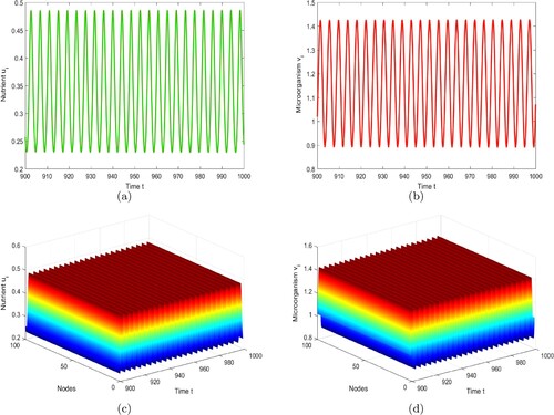
Figure 1 shows that the distribution of solutions $u_i(1\le i\le 100)$ with the development of moments. When taking time delay $0.95=\tau <{\tau }_{\ast }$, we find that the positive equilibrium $E_{\ast }$ is locally asymptotically stable, see Figure 2. Figure 3 suggests that there is a supercritical Hopf bifurcation, and the periodic solution with the spatial homogeneity bifurcated from the Hopf bifurcation is stable in the delayed network model (1), where we choose $1.1587=\tau >{\tau }_{\ast }$. As such, the results in Theorem 3.1 are valid.

Figure 1. The distribution of solution $u_i$ with the numbers $i=1,2,\dots 100$ and the connection probability p = 0.35.

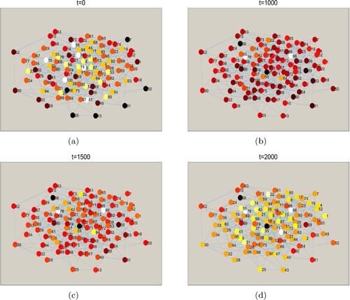
Figure 2. Positive equilibrium $E_{\ast }$ is stable when taking $0.95=\tau <{\tau }_{\ast }$ and the probability p = 0.35.

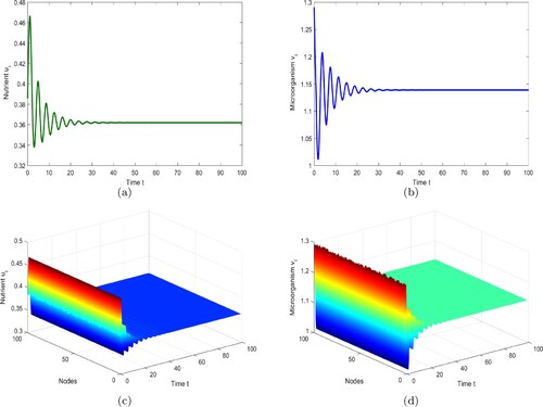
Figure 3. The delayed network model (1) admits a stable spatially homogeneous periodic solution when choosing $1.1587=\tau >{\tau }_{\ast }$ and the probability p = 0.35.

5. Conclusions

We deal with a nutrient-microorganism model with time delay and random network structure in this paper. By employing time delay τ as the critical parameter of the Hopf bifurcation, we explore its occurrence conditions. For the direction of the Hopf bifurcation, we try to adopt MTS to derive amplitude equation near $\tau ={\tau }_{\ast }$, it is found that the sign of $K_1{K}_2$ determines the existence of the Hopf bifurcation. Namely the Hopf bifurcation exists when $K_1{K}_2<0$, and there is no Hopf bifurcation when $K_1{K}_2>0$. Moreover, the sign of $K_1$ determines the direction of the Hopf bifurcation with hypothesis $K_1{K}_2<0$. More precisely, the Hopf bifurcation is supercritical (resp. subcritical) and the periodic solution is stable (resp. unstable) when $K_1>0$ (resp. $K_1<0$). Numerical simulations indicate that our theoretical analysis is valid, and compared with the works done in [9,10] we claim that MTS is a easier technique to determine the direction of the Hopf bifurcation in a delayed network model than CMR. For more interesting results about this networked model, for example, resonant/nonresonant Hopf bifurcation, will be further considered.

Disclosure statement

No potential conflict of interest was reported by the author(s).

Additional information

Funding

This work was supported by the National Natural Science Foundation of China [grant number 11971032], and Young Talent Support Project of Henan [grant number 2020HYTP012].

References

- M. Baurmann and U. Feudel, Turing patterns in a simple model of a nutrient-microorganism system in the sediment, Ecol. Complex. 1 (2004), pp. 77–94.
- M. Bentounsi, I. Agmour, and N. Achtaich, The Hopf bifurcation and stability of delayed predator-prey system, Comput. Appl. Math. 37(5) (2018), pp. 5702–5714.
- M.X. Chen, R.C. Wu, B. Liu, and L.P. Chen, Hopf-Hopf bifurcation in the delayed nutrient-microorganism model, Appl. Math. Model. 86 (2020), pp. 460–483.
- Y. Ide, H. Izuhara, and T. Machidac, Turing instability in reaction diffusion models on complex networks, Physica A. 457 (2016), pp. 331–347.
- A. Kumar and B. Dubey, Modeling the effect of fear in a prey-predator system with prey refuge and gestation delay, Int. J. Bifurcat. Chaos. 29(14) (2019), pp. 1950195.
- Y.Q. Liu, D.F. Duan, and B. Niu, Spatiotemporal dynamics in a diffusive predator prey model with group defense and nonlocal competition, Appl. Math. Lett. 103 (2020), pp. 106175.
- K. Manna and M. Banerjee, Stability of Hopf-bifurcating limit cycles in a diffusion-driven prey-predator system with Allee effect and time delay, Math. Biosci. Eng. 16(4) (2019), pp. 2411–2446.
- B. Roy, S.K. Roy, and D.B. Gurung, Holling-Tanner model with Beddington-DeAngelis functional response and time delay introducing harvesting, Math. Comput. Simul. 142 (2017), pp. 1–14.
- Y.L. Shi, Z.H. Liu, and C.R. Tian, Hopf bifurcation in an activator-inhibitor system with network, Appl. Math. Lett. 98 (2019), pp. 22–28.
- C.R. Tian, Z. Ling, and L. Zhang, Delay-driven spatial patterns in a network-organized semiarid vegetation model, Appl. Math. Comput. 367 (2020), pp. 124778.
- T.H. Zhang, Y.L. Song, and H. Zang, The stability and Hopf bifurcation analysis of a gene expression model, J. Math. Anal. Appl. 395 (2012), pp. 103–113.
- H.Y. Zhao and D.Y. Wu, Point to point traveling wave and periodic traveling wave induced by Hopf bifurcation for a diffusive predator-prey system, Discrete Cont. Dyn. Syst. S. 13(11) (2020), pp. 3271–3284.