Dynamic analysis and optimal control of a class of SISP respiratory diseases

Abstract

In this paper, the actual background of the susceptible population being directly patients after inhaling a certain amount of PM${}_{2.5}$ is taken into account. The concentration response function of PM${}_{2.5}$ is introduced, and the SISP respiratory disease model is proposed. Qualitative theoretical analysis proves that the existence, local stability and global stability of the equilibria are all related to the daily emission $P_0$ of PM${}_{2.5}$ and PM${}_{2.5}$ pathogenic threshold K. Based on the sensitivity factor analysis and time-varying sensitivity analysis of parameters on the number of patients, it is found that the conversion rate β and the inhalation rate η has the largest positive correlation. The cure rate γ of infected persons has the greatest negative correlation on the number of patients. The control strategy formulated by the analysis results of optimal control theory is as follows: The first step is to improve the clearance rate of PM${}_{2.5}$ by reducing the PM${}_{2.5}$ emissions and increasing the intensity of dust removal. Moreover, such removal work must be maintained for a long time. The second step is to improve the cure rate of patients by being treated in time. After that, people should be reminded to wear masks and go out less so as to reduce the conversion rate of susceptible people becoming patients.

Keywords:

• Respiratory disease
• PM${}_{2.5}$ emissions
• PM${}_{2.5}$ pathogenic threshold
• sensitivity analysis
• optimal control

MSC:

• 34A40
• 34C10
• 34D23
• 92B05

Highlights

• The significantdifference between this paper and other respiratory diseases models lies in that a compartment of air pollutant (PM${}_{2.5}$) is added. At the same time, the emission and pathogenic amount of PM${}_{2.5}$ are introduced, and the  emmission threshold value and pathogenic amount is given through theoretical analysis and numerical simulation. It has very important practical value for the development of public health and environmental protection.

• It is worth noting that the existence, local stability and global stability of the equilibria are all related to the daily emission $P_0$ of PM${}_{2.5}$ and PM${}_{2.5}$ pathogenic threshold K. This indicates that the emission of PM${}_{2.5}$ and the pathogenic threshold have a great impact on the transmission dynamics of respiratory diseases, which further confirms the correctness of our consideration in the model.

• This paper also proposes an optimal control strategy for the prevention and control of respiratory diseases. The first step is to improve the PM${}_{2.5}$ clearance rate. Moreover, such removal work must be maintained for a long time. The second step is to improve the cure rate. After that is to reduce the conversion rate.

1. Introduction

The rapid development of the economy has promoted the process of industrialization in China, but at the same time, it also causes serious damage to the ecological environment, and the air pollution problem has become more and more serious [22, 24, 31, 32, 44]. Meanwhile, the impact of air pollution particles on human health has also become a public health problem. Air pollution particulate matter is the fifth-ranked health risk factor in the 2017 Global Burden of Disease Assessment [7, 14]. As is known to all, the fine particulate matter (PM${}_{2.5}$) is an important part of the air pollution particulate matter. It can carry toxic and harmful substances, floating in the air for a long time, has a long transportation distance. It will enter the human body along with the breath, even into the alveoli and blood, making the respiratory system and other systems damage, leading to the occurrence of respiratory diseases and other diseases [5, 9, 12, 53]. PM${}_{2.5}$ monitoring data of major cities in China in 2016 are shown in Figure 1 [40]. It can be seen that PM${}_{2.5}$ monitoring concentration in some areas of Hebei Province is too high, indicating that local air pollution is relatively serious, the prevention and control of respiratory diseases in this region is still grim.

Figure 1. PM${}_{2.5}$ concentration in major cities in China in 2016. The data came from a WHO report in September 2020 [40].

At present, the pathogenesis, transmission rules and prevention strategies of human respiratory diseases caused by air pollution have been investigated and studied by many scholars through mathematical modelling and combining with actual data [4, 11, 16, 36]. At the same time, many epidemiological studies have shown that PM${}_{2.5}$ can avoid the nose hair, and the function of filtration by trachea cilia cells, along with the deep breathing into the respiratory tract. In addition, it can be in direct contact with human lung tissue cells, and it is difficult to fall off when adsorbed in the alveolar, causing the deposition of particulate matter. Through direct stimulation, it causes mechanical damage to the airway mucosal epithelial cells and alveolar wall, destroys the respiratory defense barrier, increases the susceptibility of the body (especially in the elderly and children with poor resistance), and aggravates the inflammatory response of respiratory diseases. In short, PM${}_{2.5}$ may cause harm to human health and even cause disease by oxide stimulation, physical and chemical reaction and mutagenesis [2, 10, 41, 49]. Therefore, it has become a hot topic to study the impact of PM${}_{2.5}$ on respiratory diseases through mathematical modelling at present.

Under normal circumstances, because of factory emissions, automobile pollution, winter heating and other reasons, air pollutants will continue to exist in the natural environment, causing harm to people's health. But the tiny particles that float in the air and can enter the lungs don't necessarily cause respiratory problems when inhaled by the body. Respiratory disease outbreaks occur only if the PM${}_{2.5}$ concentration inhaled by humans is higher than a certain critical threshold that makes susceptible people ill [23]. This critical pathogenic threshold may be caused by the clearance of the innate immune system. This kind of situation is similar to the case that the number of pathogens ingested by human beings must be higher than the critical threshold causing the infection of susceptible individuals in order to lead to the outbreak of infectious diseases [17]. In recent years, mathematical infectious disease models have been established by many scholars of introducing immune threshold or pathogen concentration threshold function to analyse the influence of such threshold on the dynamic behaviour [20, 52]. Currently, only the association between increased PM${}_{2.5}$ concentrations and increased risk of respiratory diseases has been studied in the extensive epidemiological literatures [9, 42, 54]. The specific size of PM${}_{2.5}$ pathogenic threshold and its impact on the incidence and transmission of respiratory diseases has not been explored in detail. Therefore, the concentration response function $\frac{P}{K+P}$ related to PM${}_{2.5}$ is drawn into in this paper, and a respiratory disease model with PM${}_{2.5}$ pathogenic threshold is installed and analysed.

Industrial sources, coal sources, motor vehicle sources, dust sources, biomass combustion sources, open sources are the main sources of PM${}_{2.5}$ emissions in China. These sources will emit a large amount of PM${}_{2.5}$ into the natural environment every day, which will not only affect the atmospheric environment and the ecosystem, but also cause great harm to human health [27]. PM${}_{2.5}$ emissions from the cement industry of various provinces in China in 2013 are presented in Figure 2. It can be seen that PM${}_{2.5}$ emissions of Anhui, Jiangsu, Hunan and other provinces in China this year have more than 400,000 tons [27, 47]. The amount of PM${}_{2.5}$ emission from cement industrial sources alone is already quite huge. Combined with the irregular emission from other sources, the PM${}_{2.5}$ concentration in these areas has seriously exceeded the standard. Long-term exposure of susceptible people to such seriously polluted air environment can easily lead to the outbreak of respiratory diseases [27, 29, 47]. Therefore, it has become urgent to study the influence of PM${}_{2.5}$ emissions threshold on human health through mathematical modelling.

Figure 2. PM${}_{2.5}$ emissions from cement industry in China in 2013. The data come from a IHME report in February 2020 [14].

In recent years, the impact of PM${}_{2.5}$ on respiratory diseases and human health is investigated by many scholars through using the modelling principle of infectious disease model [4, 11, 16, 36]. At the same time, on the basis of the traditional infectious disease model, the compartment of virus or bacterial population is added by many scholars to study the propagation dynamics of the model [1, 3, 6, 19, 28, 34, 39, 50]. However, little literature has brought the compartment of PM${}_{2.5}$ in respiratory disease models to establish relevant mathematical models for analysis and research. Inspired by this, based on the our previous work [33], a new compartment is added to describe the dynamic behaviour of PM${}_{2.5}$, and a three-dimensional SISP respiratory disease model is proposed in this paper to study the impact of PM${}_{2.5}$ emissions on the outbreak and spread of respiratory diseases.

The structure of this article as follows: In Section 2, the SISP respiratory disease model is built in which the susceptible population directly got sick after inhaling PM${}_{2.5}$. In Section 3, the boundedness of the solution, the existence and stability of the equilibria are investigated. In Section 4, the sensitivity of parameters to the number of patients is presented. Section 5 is the optimal control analysis. Section 6 is the numerical simulation. Result and discussion are given at the end.

2. Mathematical modelling

In actual life, major emission source emit large amounts of PM${}_{2.5}$ into the air daily, and let $P_0$ denote the daily emissions. The respiratory systems of susceptible people exposed to such polluted air can be damaged by inhaling PM${}_{2.5}$, which can lead to respiratory diseases and make susceptible people become patients directly [5, 9, 12, 53]. In addition, a trace amount of PM${}_{2.5}$ will not cause great harm to the human body due to the role of autoimmune function. Respiratory disease outbreaks only when the PM${}_{2.5}$ concentration is higher than some pathogenic threshold K [9, 23, 42, 54]. In this paper, the following SISP respiratory disease model is built by integrating the above two actual situations: (1) $\{\begin{array}{l}{\displaystyle \frac{\mathrm{d}S}{\mathrm{d}t}}=\mathrm{\Lambda }-\mu S+\gamma I-{\displaystyle \frac{\text{β}\eta SP}{K+P}},\\ {\displaystyle \frac{\mathrm{d}I}{\mathrm{d}t}}={\displaystyle \frac{\text{β}\eta SP}{K+P}}-\mu I-\alpha I-\gamma I,\\ {\displaystyle \frac{\mathrm{d}P}{\mathrm{d}t}}=P_0-cP-\eta (S+I).\end{array}$(1) Where, S represents the number of susceptible people, I represents the number of infected people, and P represents the PM${}_{2.5}$ concentration. Λ is the recruitment rate of susceptible persons, μ is the natural mortality rate of susceptible and infected persons, α is the disease-induced mortality rate of infected persons, and γ is the cure rate of infected persons, β is the conversion rate of susceptible individuals become patients by inhaling PM${}_{2.5}$. $\frac{P}{K+P}$ is the concentration response function related to PM${}_{2.5}$, representing the probability of each susceptible person getting sick by inhaling PM${}_{2.5}$. c is the clearance rate for PM${}_{2.5}$, and η is the inhalation rate for PM${}_{2.5}$ per person.

3. Qualitative analysis

3.1. Boundedness of solutions

Theorem 3.1

The solutions $(S_0,I_0,P_0)$ of system (2.1) with initial value $S\left(0\right)>0,I\left(0\right)\ge 0,P\left(0\right)>0$ are positive for all $t>0$. All solutions of system (2.1) are uniformly bounded on $\mathrm{\Omega }=\{(S,I,P)R_{+}^3:0\le S+I=N\le \frac{\mathrm{\Lambda }}{\mu },0\le P\le \frac{P_0}{c}\}.$

Proof.

First, the total derivative of the function $N\left(t\right)=S\left(t\right)+I\left(t\right)$ along the solution of system (1(1) $\{\begin{array}{l}{\displaystyle \frac{\mathrm{d}S}{\mathrm{d}t}}=\mathrm{\Lambda }-\mu S+\gamma I-{\displaystyle \frac{\text{β}\eta SP}{K+P}},\\ {\displaystyle \frac{\mathrm{d}I}{\mathrm{d}t}}={\displaystyle \frac{\text{β}\eta SP}{K+P}}-\mu I-\alpha I-\gamma I,\\ {\displaystyle \frac{\mathrm{d}P}{\mathrm{d}t}}=P_0-cP-\eta (S+I).\end{array}$(1) ) can be obtained, we have $\frac{\mathrm{d}N\left(t\right)}{\mathrm{d}t}=\frac{\mathrm{d}S\left(t\right)}{\mathrm{d}t}+\frac{\mathrm{d}I\left(t\right)}{\mathrm{d}t}=\mathrm{\Lambda }-\mu [S\left(t\right)+I\left(t\right)]-\alpha I\left(t\right)\le \mathrm{\Lambda }-\mu N\left(t\right).$So, we get $N\left(t\right)\le \frac{\mathrm{\Lambda }}{\mu }-(\frac{\mathrm{\Lambda }}{\mu }-N(0\left)\right)e^{-\mu t}$ for all $t\ge 0$. Hence, $\underset{t\to \mathrm{\infty }}{lim}supN\left(t\right)\le \frac{\mathrm{\Lambda }}{\mu }$.

From the third equation of system (1(1) $\{\begin{array}{l}{\displaystyle \frac{\mathrm{d}S}{\mathrm{d}t}}=\mathrm{\Lambda }-\mu S+\gamma I-{\displaystyle \frac{\text{β}\eta SP}{K+P}},\\ {\displaystyle \frac{\mathrm{d}I}{\mathrm{d}t}}={\displaystyle \frac{\text{β}\eta SP}{K+P}}-\mu I-\alpha I-\gamma I,\\ {\displaystyle \frac{\mathrm{d}P}{\mathrm{d}t}}=P_0-cP-\eta (S+I).\end{array}$(1) ), it can be known $\frac{\mathrm{d}P\left(t\right)}{\mathrm{d}t}=P_0-cP\left(t\right)-\eta [S\left(t\right)+I\left(t\right)]\le P_0-cP\left(t\right).$Hence, we can obtain $P\left(t\right)\le \frac{P_0}{c}-(\frac{P_0}{c}-P(0\left)\right)e^{-ct}$ for all $t\ge 0$. Therefore $\underset{t\to \mathrm{\infty }}{lim}supP\left(t\right)\le \frac{P_0}{c}$.

To sum up, it can be concluded that the positive invariant set of system (1(1) $\{\begin{array}{l}{\displaystyle \frac{\mathrm{d}S}{\mathrm{d}t}}=\mathrm{\Lambda }-\mu S+\gamma I-{\displaystyle \frac{\text{β}\eta SP}{K+P}},\\ {\displaystyle \frac{\mathrm{d}I}{\mathrm{d}t}}={\displaystyle \frac{\text{β}\eta SP}{K+P}}-\mu I-\alpha I-\gamma I,\\ {\displaystyle \frac{\mathrm{d}P}{\mathrm{d}t}}=P_0-cP-\eta (S+I).\end{array}$(1) ) is $\mathrm{\Omega }=\{(S,I,P)R_{+}^3:0\le S+I=N\le \frac{\mathrm{\Lambda }}{\mu },0\le P\le \frac{P_0}{c}\}.\text{■}$

3.2. Existence of equilibria

Theorem 3.2

For system (1(1) $\{\begin{array}{l}{\displaystyle \frac{\mathrm{d}S}{\mathrm{d}t}}=\mathrm{\Lambda }-\mu S+\gamma I-{\displaystyle \frac{\text{β}\eta SP}{K+P}},\\ {\displaystyle \frac{\mathrm{d}I}{\mathrm{d}t}}={\displaystyle \frac{\text{β}\eta SP}{K+P}}-\mu I-\alpha I-\gamma I,\\ {\displaystyle \frac{\mathrm{d}P}{\mathrm{d}t}}=P_0-cP-\eta (S+I).\end{array}$(1) ), we have:

1. There is a disease-free equilibrium $E_0=(S_0,0,0)$ if $P_0=\eta \frac{\mathrm{\Lambda }}{\mu }$, here $S_0=\frac{P_0}{\eta }=\frac{\mathrm{\Lambda }}{\mu }$.

2. There is no endemic equilibrium if $K>K_1$, here $K_1=\frac{{\{\sqrt{(\eta \mathrm{\Lambda }-\mu P_0)[\text{β}\eta (\mu +\alpha )+\mu (\mu +\alpha +\gamma )]}-\sqrt{\text{β}{\eta }^2\mathrm{\Lambda }\alpha }\}}^2}{c{\mu }^2(\mu +\alpha +\gamma )}.$

3. There is unique endemic equilibrium $E_1^{\ast }=(S_1^{\ast },I_1^{\ast },P_1^{\ast })$ if $P_0<\eta \frac{\mathrm{\Lambda }}{\mu }$, $K=K_1$, where $\begin{array}{rl}{S}_1^{\ast }& =\frac{\mathrm{\Lambda }-(\mu +\alpha )I_1^{\ast }}{\mu },P_1^{\ast }=\frac{\mu P_0-\eta \mathrm{\Lambda }+\eta \alpha I_1^{\ast }}{\mu c},\\ I_1^{\ast }& =\frac{\begin{array}{c}\eta \mathrm{\Lambda }[\text{β}\eta (\mu +2\alpha )+\mu (\mu +\alpha +\gamma )]\\ -[\text{β}\eta \mu P_0(\mu +\alpha )+{\mu }^2(\mu +\alpha +\gamma )(cK+P_0)]\end{array}}{2\eta \alpha [\text{β}\eta (\mu +\alpha )+\mu (\mu +\alpha +\gamma )]}>0.\end{array}$

4. There is an endemic equilibrium $E_2^{\ast }=(S_2^{\ast },I_2^{\ast },P_2^{\ast })$ if $\eta \frac{\mathrm{\Lambda }}{\mu }<P_0<\eta \frac{\mathrm{\Lambda }}{\mu }(1+\frac{\alpha }{\mu +\alpha })$, where $\begin{array}{rl}{S}_2^{\ast }& =\frac{\mathrm{\Lambda }-(\mu +\alpha )I_2^{\ast }}{\mu },P_2^{\ast }=\frac{\mu P_0-\eta \mathrm{\Lambda }+\eta \alpha I_2^{\ast }}{\mu c},\\ I_2^{\ast }& =\frac{\begin{array}{c}[\text{β}\eta \mu P_0(\mu +\alpha )+{\mu }^2(\mu +\alpha +\gamma )(cK+P_0)\\ -\eta \mathrm{\Lambda }[\text{β}\eta (\mu +2\alpha )+\mu (\mu +\alpha +\gamma )]\phantom{{\mu }^2}]+\sqrt{\mathrm{\Delta }}\end{array}}{2\eta \alpha [\text{β}\eta (\mu +\alpha )+\mu (\mu +\alpha +\gamma )]}>0.\end{array}$

5. There are two different endemic equilibria $E_2^{\ast }=(S_2^{\ast },I_2^{\ast },P_2^{\ast })$ and $E_3^{\ast }=(S_3^{\ast },I_3^{\ast },P_3^{\ast })$ if $P_0<\eta \frac{\mathrm{\Lambda }}{\mu }$, $K_5<K<K_1$, where $\begin{array}{rl}{K}_5& =\frac{(\eta \mathrm{\Lambda }-\mu P_0)[\text{β}\eta (\mu +\alpha )+\mu (\mu +\alpha +\gamma )]}{c{\mu }^2(\mu +\alpha +\gamma )},\\ S_3^{\ast }& =\frac{\mathrm{\Lambda }-(\mu +\alpha )I_3^{\ast }}{\mu },P_3^{\ast }=\frac{\mu P_0-\eta \mathrm{\Lambda }+\eta \alpha I_3^{\ast }}{\mu c},\\ I_3^{\ast }& =\frac{\begin{array}{c}[\text{β}\eta \mu P_0(\mu +\alpha )+{\mu }^2(\mu +\alpha +\gamma )(cK+P_0)\\ -\eta \mathrm{\Lambda }[\text{β}\eta (\mu +2\alpha )+\mu (\mu +\alpha +\gamma )]\phantom{{\mu }^2}]-\sqrt{\mathrm{\Delta }}\end{array}}{2\eta \alpha [\text{β}\eta (\mu +\alpha )+\mu (\mu +\alpha +\gamma )]}>0.\end{array}$

Proof.

To solve the equilibrium of system (1(1) $\{\begin{array}{l}{\displaystyle \frac{\mathrm{d}S}{\mathrm{d}t}}=\mathrm{\Lambda }-\mu S+\gamma I-{\displaystyle \frac{\text{β}\eta SP}{K+P}},\\ {\displaystyle \frac{\mathrm{d}I}{\mathrm{d}t}}={\displaystyle \frac{\text{β}\eta SP}{K+P}}-\mu I-\alpha I-\gamma I,\\ {\displaystyle \frac{\mathrm{d}P}{\mathrm{d}t}}=P_0-cP-\eta (S+I).\end{array}$(1) ), let $\{\begin{array}{l}\mathrm{\Lambda }-\mu S+\gamma I-{\displaystyle \frac{\text{β}\eta SP}{K+P}}=0,\\ {\displaystyle \frac{\text{β}\eta SP}{K+P}}-\mu I-\alpha I-\gamma I=0,\\ P_0-cP-\eta (S+I)=0.\end{array}$If P = 0, and I = 0, then $S=\frac{P_0}{\eta }=\frac{\mathrm{\Lambda }}{\mu }$. Hence, system (1(1) $\{\begin{array}{l}{\displaystyle \frac{\mathrm{d}S}{\mathrm{d}t}}=\mathrm{\Lambda }-\mu S+\gamma I-{\displaystyle \frac{\text{β}\eta SP}{K+P}},\\ {\displaystyle \frac{\mathrm{d}I}{\mathrm{d}t}}={\displaystyle \frac{\text{β}\eta SP}{K+P}}-\mu I-\alpha I-\gamma I,\\ {\displaystyle \frac{\mathrm{d}P}{\mathrm{d}t}}=P_0-cP-\eta (S+I).\end{array}$(1) ) has a disease-free equilibrium $E_0=(S_0,0,0)$, where $S_0=\frac{P_0}{\eta }=\frac{\mathrm{\Lambda }}{\mu }$.

Add the first and second equations to get $S=\frac{\mathrm{\Lambda }-(\mu +\alpha )I}{\mu }$. So we obtain $P=\frac{\mu P_0-\eta \mathrm{\Lambda }+\eta \alpha I}{\mu c}$ from the third equation.

Substituting these two equations into the first equation, one has (2) $A{I}^2+BI+C=0,$(2) where

$A=\eta \alpha \left[\text{β}\eta \right(\mu +\alpha )+\mu (\mu +\alpha +\gamma \left)\right],$

$B=\left[\text{β}\eta \mu P_0\right(\mu +\alpha )+{\mu }^2(\mu +\alpha +\gamma \left)\right(cK+P_0\left)\right]-\eta \mathrm{\Lambda }\left[\text{β}\eta \right(\mu +2\alpha )+\mu (\mu +\alpha +\gamma \left)\right]$,

$C=\text{β}\eta \mathrm{\Lambda }(\eta \mathrm{\Lambda }-\mu P_0)$,

$\mathrm{\Delta }=\left\{\right[\text{β}\eta \mu P_0(\mu +\alpha )+{\mu }^2(\mu +\alpha +\gamma )(cK+P_0)]-\eta \mathrm{\Lambda }[\text{β}\eta (\mu +2\alpha )+\mu (\mu +\alpha +\gamma )]{\}}^2$ $-4\text{β}{\eta }^2\mathrm{\Lambda }\alpha (\eta \mathrm{\Lambda }-\mu P_0)[\text{β}\eta (\mu +\alpha )+\mu (\mu +\alpha +\gamma )].$To take the existence of the endemic equilibrium $E^{\ast }=(S^{\ast },I^{\ast },P^{\ast })$, then $S^{\ast }$, $P^{\ast }$ must be positive, and the roots $I^{\ast }$ of the quadratic Equation (2(2) $A{I}^2+BI+C=0,$(2) ) must also be positive. Therefore, the quadratic Equation (2(2) $A{I}^2+BI+C=0,$(2) ) has no real roots if $\mathrm{\Delta }<0$. The quadratic Equation (2(2) $A{I}^2+BI+C=0,$(2) ) has one real root $I_1^{\ast }=-\frac{B}{2A}>0(B<0)$ if $\mathrm{\Delta }<0$. The quadratic equation (2(2) $A{I}^2+BI+C=0,$(2) ) has two different real roots $I_2^{\ast }=\frac{-B+\sqrt{\mathrm{\Delta }}}{2A}$ and $I_3^{\ast }=\frac{-B-\sqrt{\mathrm{\Delta }}}{2A}$ when $\mathrm{\Delta }>0$.

Let's simplify the Equation (2(2) $A{I}^2+BI+C=0,$(2) ) to $A{I}^2+C=-BI$, and then the existence of the equilibrium in system (1(1) $\{\begin{array}{l}{\displaystyle \frac{\mathrm{d}S}{\mathrm{d}t}}=\mathrm{\Lambda }-\mu S+\gamma I-{\displaystyle \frac{\text{β}\eta SP}{K+P}},\\ {\displaystyle \frac{\mathrm{d}I}{\mathrm{d}t}}={\displaystyle \frac{\text{β}\eta SP}{K+P}}-\mu I-\alpha I-\gamma I,\\ {\displaystyle \frac{\mathrm{d}P}{\mathrm{d}t}}=P_0-cP-\eta (S+I).\end{array}$(1) ) is discussed by using the symbolic-graphic combination.

1. There is only one intersection between functions $f_1\left(I\right)=A{I}^2+C$ and $f_2\left(I\right)=-BI$ on the right side of I if B>0, C>0.

2. There is no intersection between functions $f_1\left(I\right)$ and $f_2\left(I\right)$ on the right side of I if B<0, C>0 and Δ. There is an intersection $I_1^{\ast }=\frac{-B}{2A}>0$ between functions $f_1\left(I\right)$ and $f_2\left(I\right)$ if $\mathrm{\Delta }=0$. There are two intersections $I_2^{\ast }=\frac{-B+\sqrt{\mathrm{\Delta }}}{2A}$ and $I_3^{\ast }=\frac{-B-\sqrt{\mathrm{\Delta }}}{2A}$ between functions $f_1\left(I\right)$ and $f_2\left(I\right)$ if Δ.

3. There is only one intersection $I_2^{\ast }=\frac{-B+\sqrt{\mathrm{\Delta }}}{2A}$ between functions $f_1\left(I\right)$ and $f_2\left(I\right)$ on the right side of I if B>0, C<0.

4. There is only one intersection $I_2^{\ast }=\frac{-B+\sqrt{\mathrm{\Delta }}}{2A}$ between functions $f_1\left(I\right)$ and $f_2\left(I\right)$ on the right side of I if B<0, C<0.

From what has been discussed above, we can draw the following conclusion:

1. System (1(1) $\{\begin{array}{l}{\displaystyle \frac{\mathrm{d}S}{\mathrm{d}t}}=\mathrm{\Lambda }-\mu S+\gamma I-{\displaystyle \frac{\text{β}\eta SP}{K+P}},\\ {\displaystyle \frac{\mathrm{d}I}{\mathrm{d}t}}={\displaystyle \frac{\text{β}\eta SP}{K+P}}-\mu I-\alpha I-\gamma I,\\ {\displaystyle \frac{\mathrm{d}P}{\mathrm{d}t}}=P_0-cP-\eta (S+I).\end{array}$(1) ) has a disease-free equilibrium $E_0=(S_0,0,0)$ if $P_0=\eta \frac{\mathrm{\Lambda }}{\mu }$, and the factory emissions threshold is recorded as $P_0$, where $S_0=\frac{P_0}{\eta }=\frac{\mathrm{\Lambda }}{\mu }$.

2. When $P_0\ne \eta \frac{\mathrm{\Lambda }}{\mu }$, two cases discussed below:

   1. When $P_0>\eta \frac{\mathrm{\Lambda }}{\mu }(C<0)$, system has an endemic equilibrium $E_2^{\ast }=(S_2^{\ast },I_2^{\ast },P_2^{\ast })$ if $\mathrm{\Delta }>0$, $\mathrm{\Lambda }-(\mu +\alpha )I_2^{\ast }>0$, $\mu P_0-\eta \mathrm{\Lambda }+\eta \alpha I_2^{\ast }>0$.We know that $\mathrm{\Delta }>0$ and $\mathrm{\Lambda }-(\mu +\alpha )I_2^{\ast }>0$ are always true. And $\mu P_0-\eta \mathrm{\Lambda }+\eta \alpha I_2^{\ast }>0$ is always true from $P_0>\eta \frac{\mathrm{\Lambda }}{\mu }$.Then, we have $I_2^{\ast }<\frac{\mathrm{\Lambda }}{\mu +\alpha }$ by $\mathrm{\Lambda }-(\mu +\alpha )I_2^{\ast }>0$. Therefore, $I_2^{\ast }$ is meaningful if and only if $\frac{\mathrm{\Lambda }}{\mu +\alpha }>\frac{\mu P_0-\eta \mathrm{\Lambda }}{\eta \alpha }$ is true, and then there is an endemic equilibrium $E_2^{\ast }$. So $\eta \frac{\mathrm{\Lambda }}{\mu }<P_0<\eta \frac{\mathrm{\Lambda }}{\mu }(1+\frac{\alpha }{\mu +\alpha })$ is a guarantee that $\frac{\mathrm{\Lambda }}{\mu +\alpha }>\frac{\mu P_0-\eta \mathrm{\Lambda }}{\eta \alpha }$ is always true.Hence, system (1(1) $\{\begin{array}{l}{\displaystyle \frac{\mathrm{d}S}{\mathrm{d}t}}=\mathrm{\Lambda }-\mu S+\gamma I-{\displaystyle \frac{\text{β}\eta SP}{K+P}},\\ {\displaystyle \frac{\mathrm{d}I}{\mathrm{d}t}}={\displaystyle \frac{\text{β}\eta SP}{K+P}}-\mu I-\alpha I-\gamma I,\\ {\displaystyle \frac{\mathrm{d}P}{\mathrm{d}t}}=P_0-cP-\eta (S+I).\end{array}$(1) ) has only one endemic equilibrium when $\eta \frac{\mathrm{\Lambda }}{\mu }<P_0<\eta \frac{\mathrm{\Lambda }}{\mu }(1+\frac{\alpha }{\mu +\alpha })$.

   2. When $P_0<\eta \frac{\mathrm{\Lambda }}{\mu }(C>0)$, there are two cases: $\begin{array}{rl}(\mid )\text{ There is an endemic equilibrium}{E}_1^{\ast }& =(S_1^{\ast },I_1^{\ast },P_1^{\ast })\mathrm{i}\mathrm{f}B<0,\\ \mathrm{\Delta }& =0,\{\begin{array}{l}\mathrm{\Lambda }-(\mu +\alpha )I_1^{\ast }>0\\ \mu P_0-\eta \mathrm{\Lambda }+\eta \alpha I_1^{\ast }>0\end{array}.\end{array}$ We can acquire $K_1=\frac{\{\sqrt{(\eta \mathrm{\Lambda }-\mu P_0)\left[\text{β}\eta \right(\mu +\alpha )+\mu (\mu +\alpha +\gamma \left)\right]}-\sqrt{\text{β}{\eta }^2\mathrm{\Lambda }\alpha }{\}}^2}{c{\mu }^2(\mu +\alpha +\gamma )}$ from $\mathrm{\Delta }=0$.

   And then we have $K<\frac{\text{β}{\eta }^2\mathrm{\Lambda }\alpha +(\eta \mathrm{\Lambda }-\mu P_0)\left[\text{β}\eta \right(\mu +\alpha )+\mu (\mu +\alpha +\gamma \left)\right]}{c{\mu }^2(\mu +\alpha +\gamma )}=K_2$ from B<0.

   According to $\mathrm{\Lambda }-(\mu +\alpha )I_1^{\ast }>0$ and $P_0<\eta \frac{\mathrm{\Lambda }}{\mu }$, one has $\begin{array}{rl}& {\eta }^2\mathrm{\Lambda }\text{β}\alpha (\mu +\alpha )+2\eta \mathrm{\Lambda }\mu \alpha (\mu +\alpha +\gamma )+{\mu }^2(\mu +\alpha )(\mu +\alpha +\gamma )cK\\ & >(\eta \mathrm{\Lambda }-\mu P_0)[\text{β}\eta {(\mu +\alpha )}^2+\mu (\mu +\alpha )(\mu +\alpha +\gamma )]\\ & >(\eta \mathrm{\Lambda }-\mu \mathrm{\Lambda }\frac{\eta }{\mu })[\text{β}\eta {(\mu +\alpha )}^2+\mu (\mu +\alpha )(\mu +\alpha +\gamma )]=0.\end{array}$

Then, $P_0<\eta \frac{\mathrm{\Lambda }}{\mu }$ guarantees that $\mathrm{\Lambda }-(\mu +\alpha )I_1^{\ast }>0$ is always true.

And then we get $K<\frac{\text{β}{\eta }^2\mathrm{\Lambda }\alpha +\eta (\mathrm{\Lambda }+2\eta \alpha )\left[\text{β}\eta \right(\mu +\alpha )+\mu (\mu +\alpha +\gamma \left)\right]}{c{\mu }^2(\mu +\alpha +\gamma )}=K_3$ from $\mu P_0-\eta \mathrm{\Lambda }+\eta \alpha I_1^{\ast }>0$.

In addition, we have $K=K_1$ from $K<min\{K_2,K_3\}=K_2$ and $K=K_1<K_2$.

Hence, system has an endemic equilibrium $E_1^{\ast }$ if $P_0<\eta \frac{\mathrm{\Lambda }}{\mu }$, $K=K_1$.

$(\parallel )$ There are two distinct endemic equilibria $E_2^{\ast }=(S_2^{\ast },I_2^{\ast },P_2^{\ast })$ and $E_3^{\ast }=(S_3^{\ast },I_3^{\ast },P_3^{\ast })$ if B<0, $\mathrm{\Delta }>0,\{\begin{array}{l}\mathrm{\Lambda }-(\mu +\alpha )I_2^{\ast }>0\\ \mu P_0-\eta \mathrm{\Lambda }+\eta \alpha I_2^{\ast }>0\end{array}\mathrm{a}\mathrm{n}\mathrm{d}\{\begin{array}{l}\mathrm{\Lambda }-(\mu +\alpha )I_3^{\ast }>0\\ \mu P_0-\eta \mathrm{\Lambda }+\eta \alpha I_3^{\ast }>0\end{array}.$According to B<0, we get $K<\frac{\text{β}{\eta }^2\mathrm{\Lambda }\alpha +(\eta \mathrm{\Lambda }-\mu P_0)\left[\text{β}\eta \right(\mu +\alpha )+\mu (\mu +\alpha +\gamma \left)\right]}{c{\mu }^2(\mu +\alpha +\gamma )}=K_2$.

From $\mathrm{\Delta }>0$ and $P_0<\eta \frac{\mathrm{\Lambda }}{\mu }$, one has $\begin{array}{rl}\mathrm{\Delta }& =\left\{\right[\text{β}\eta \mu P_0(\mu +\alpha )+{\mu }^2(\mu +\alpha +\gamma )(cK+P_0)]\\ & -\eta \mathrm{\Lambda }\left[\text{β}\eta \right(\mu +2\alpha )+\mu (\mu +\alpha +\gamma \left)\right]{\}}^2\\ & >4\text{β}{\eta }^2\mathrm{\Lambda }\alpha (\eta \mathrm{\Lambda }-\mu P_0)[\text{β}\eta (\mu +\alpha )+\mu (\mu +\alpha +\gamma )]\\ & >4\text{β}{\eta }^2\mathrm{\Lambda }\alpha (\eta \mathrm{\Lambda }-\mu \eta \frac{\mathrm{\Lambda }}{\mu })[\text{β}\eta (\mu +\alpha )+\mu (\mu +\alpha +\gamma )]=0.\end{array}$Then, $P_0<\eta \frac{\mathrm{\Lambda }}{\mu }$ is the guarantee that $\mathrm{\Delta }>0$ is always true.

According to C>0, we have $\mu P_0-\eta \mathrm{\Lambda }+\eta \alpha I_2^{\ast }>0$. Meanwhile $\mu P_0-\eta \mathrm{\Lambda }+\eta \alpha I_3^{\ast }>0$ by $I_2^{\ast }>I_3^{\ast }$.

On the basis of $\mu P_0-\eta \mathrm{\Lambda }+\eta \alpha I_2^{\ast }>0$, we obtain $K<\frac{(\eta \mathrm{\Lambda }-\mu P_0)[\text{β}\eta (\mu +\alpha )+\mu (\mu +\alpha +\gamma )]+(\eta \mathrm{\Lambda }-\mu P_0)}{c{\mu }^2(\mu +\alpha +\gamma )}=K_4.$From $\mu P_0-\eta \mathrm{\Lambda }+\eta \alpha I_3^{\ast }>0$, we have $K>\frac{(\eta \mathrm{\Lambda }-\mu P_0)\left[\text{β}\eta \right(\mu +\alpha )+\mu (\mu +\alpha +\gamma \left)\right]}{c{\mu }^2(\mu +\alpha +\gamma )}=K_5$.

Moreover, $K_5<K<min\{K_2,K_4\}=K_4$. Comprehensive analysis shows that, system (1(1) $\{\begin{array}{l}{\displaystyle \frac{\mathrm{d}S}{\mathrm{d}t}}=\mathrm{\Lambda }-\mu S+\gamma I-{\displaystyle \frac{\text{β}\eta SP}{K+P}},\\ {\displaystyle \frac{\mathrm{d}I}{\mathrm{d}t}}={\displaystyle \frac{\text{β}\eta SP}{K+P}}-\mu I-\alpha I-\gamma I,\\ {\displaystyle \frac{\mathrm{d}P}{\mathrm{d}t}}=P_0-cP-\eta (S+I).\end{array}$(1) ) has two endemic equilibria $E_2^{\ast }$ and $E_3^{\ast }$ if $P_0<\eta \frac{\mathrm{\Lambda }}{\mu }$, $K_5<K<K_1$.

According to the analysis results in Table 1 and Figure 3 above, it can be seen that the existence of the equilibria of the system (1(1) $\{\begin{array}{l}{\displaystyle \frac{\mathrm{d}S}{\mathrm{d}t}}=\mathrm{\Lambda }-\mu S+\gamma I-{\displaystyle \frac{\text{β}\eta SP}{K+P}},\\ {\displaystyle \frac{\mathrm{d}I}{\mathrm{d}t}}={\displaystyle \frac{\text{β}\eta SP}{K+P}}-\mu I-\alpha I-\gamma I,\\ {\displaystyle \frac{\mathrm{d}P}{\mathrm{d}t}}=P_0-cP-\eta (S+I).\end{array}$(1) ) is influenced by the daily emission of PM${}_{2.5}$ and the PM${}_{2.5}$ pathogenic threshold. That is to say, by adjusting the PM${}_{2.5}$ pathogenic threshold K and the daily emission $P_0$ of PM${}_{2.5}$, the existence of endemic equilibrium in the system can be controlled, so that system only has the disease-free equilibrium as far as possible, so as to reduce the harm of PM${}_{2.5}$ and achieve the purpose of controlling the spread of respiratory diseases.

Figure 3. Existence of the equilibria in system (1(1) $\{\begin{array}{l}{\displaystyle \frac{\mathrm{d}S}{\mathrm{d}t}}=\mathrm{\Lambda }-\mu S+\gamma I-{\displaystyle \frac{\text{β}\eta SP}{K+P}},\\ {\displaystyle \frac{\mathrm{d}I}{\mathrm{d}t}}={\displaystyle \frac{\text{β}\eta SP}{K+P}}-\mu I-\alpha I-\gamma I,\\ {\displaystyle \frac{\mathrm{d}P}{\mathrm{d}t}}=P_0-cP-\eta (S+I).\end{array}$(1) ), here $P_1=\eta \frac{\mathrm{\Lambda }}{\mu }$, $P_2=\eta \frac{\mathrm{\Lambda }}{\mu }(1+\frac{\alpha }{\mu +\alpha })$.

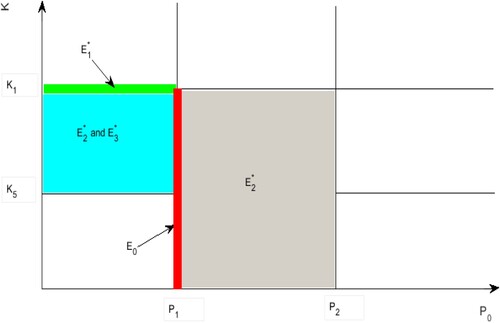
Table 1. Existence of the equilibria in system (1(1) $\{\begin{array}{l}{\displaystyle \frac{\mathrm{d}S}{\mathrm{d}t}}=\mathrm{\Lambda }-\mu S+\gamma I-{\displaystyle \frac{\text{β}\eta SP}{K+P}},\\ {\displaystyle \frac{\mathrm{d}I}{\mathrm{d}t}}={\displaystyle \frac{\text{β}\eta SP}{K+P}}-\mu I-\alpha I-\gamma I,\\ {\displaystyle \frac{\mathrm{d}P}{\mathrm{d}t}}=P_0-cP-\eta (S+I).\end{array}$(1) ).

$P_0$	K	Equilibria
$P_0=\eta {\displaystyle \frac{\mathrm{\Lambda }}{\mu }}$	–	Disease free equilibrium $E_0$
$P_0<\eta {\displaystyle \frac{\mathrm{\Lambda }}{\mu }}$	$K_5<K<K_1$	Endemic equilibria $E_2^{\ast }$ and $E_3^{\ast }$
	$K=K_1$	Endemic equilibrium $E_1^{\ast }$
$\eta {\displaystyle \frac{\mathrm{\Lambda }}{\mu }}<P_0<\eta {\displaystyle \frac{\mathrm{\Lambda }}{\mu }}(1+{\displaystyle \frac{\alpha }{\mu +\alpha }})$	–	Endemic equilibrium $E_2^{\ast }$

3.3. Local stability analysis

3.3.1. Local stability of disease-free equilibrium $E_0$ when $P_0=\eta \frac{\mathrm{\Lambda }}{\mu }$

Theorem 3.3

The disease-free equilibrium $E_0$ is locally asymptotically stable when $K>\frac{\text{β}{\eta }^2\mathrm{\Lambda }\alpha }{c{\mu }^2(\mu +\alpha +\gamma )}$.

Proof.

The Jacobian matrix of system (1(1) $\{\begin{array}{l}{\displaystyle \frac{\mathrm{d}S}{\mathrm{d}t}}=\mathrm{\Lambda }-\mu S+\gamma I-{\displaystyle \frac{\text{β}\eta SP}{K+P}},\\ {\displaystyle \frac{\mathrm{d}I}{\mathrm{d}t}}={\displaystyle \frac{\text{β}\eta SP}{K+P}}-\mu I-\alpha I-\gamma I,\\ {\displaystyle \frac{\mathrm{d}P}{\mathrm{d}t}}=P_0-cP-\eta (S+I).\end{array}$(1) ) evaluated at the equilibrium $E_0$ is given by $J\left(E_0\right)=\left(\begin{array}{ccc}-\mu & \gamma & -{\displaystyle \frac{\text{β}\eta S_0}{K}}\\ 0& -(\mu +\alpha +\gamma )& {\displaystyle \frac{\text{β}\eta S_0}{K}}\\ -\eta & -\eta & -c\end{array}\right).$The corresponding characteristic equation is $det(\lambda I-J\left(E_0\right))={\lambda }^3+A_1{\lambda }^2+A_2\lambda +A_3=0,$where

$A_1=(\mu +\alpha +\gamma )+\mu +c>0$,

$A_2=(c+\mu )(\mu +\alpha +\gamma )+c\mu >0$,

$A_3=c\mu (\mu +\alpha +\gamma )-\eta \frac{\text{β}\eta S_0}{K}\alpha$.

When $c\mu (\mu +\alpha +\gamma )-\eta \frac{\text{β}\eta S_0}{K}\alpha >0$, that $K>\frac{\text{β}{\eta }^2\mathrm{\Lambda }\alpha }{c{\mu }^2(\mu +\alpha +\gamma )}$, we have $A_3>0$.

Then, the sign of the real part of the eigenvalues is discussed using the Routh–Hurtwitz criterion [13, 25]. Let $H_1=A_1,H_2=\left|\begin{array}{cc}{A}_1& A_3\\ 1& A_2\end{array}\right|,H_3=\left|\begin{array}{ccc}{A}_1& A_3& 0\\ 1& A_2& 0\\ 0& A_1& A_3\end{array}\right|.$Thus, we get

$H_1=A_1=(\mu +\alpha +\gamma )+\mu +c>0$,

$H_2=A_1{A}_2-A_3=(c+\mu )(\mu +\alpha +\gamma )\left[\right(\mu +\alpha +\gamma )+(c+\mu \left)\right]+c\mu (c+\mu )+\eta \frac{\text{β}\eta S_0}{K}\alpha >0$,

$H_3=A_3{H}_2>0$.

According to the Routh–Hurtwitz criterion, if $K>\frac{\text{β}{\eta }^2\mathrm{\Lambda }\alpha }{c{\mu }^2(\mu +\alpha +\gamma )}$, then the real parts of all eigenvalues of $E_0$ are negative. Therefore, $E_0$ is locally asymptotically stable. Theorem 3.3 can be obtained from the existence condition of disease-free equilibrium $E_0$.

3.3.2. Local stability of endemic equilibrium $E_1^{\ast }$ when $P_0<\eta \frac{\mathrm{\Lambda }}{\mu }$, $K=K_1$

Theorem 3.4

The endemic equilibrium $E_1^{\ast }$ is locally asymptotically stable when $P_0>\overline{P}$, where $\overline{P}=\eta \frac{\mathrm{\Lambda }}{\mu }\cdot \frac{\text{β}\eta \alpha }{\mu (\mu +\alpha +\gamma )}$.

Proof.

The Jacobian matrix corresponding to the endemic equilibrium $E_1^{\ast }$ of system (1(1) $\{\begin{array}{l}{\displaystyle \frac{\mathrm{d}S}{\mathrm{d}t}}=\mathrm{\Lambda }-\mu S+\gamma I-{\displaystyle \frac{\text{β}\eta SP}{K+P}},\\ {\displaystyle \frac{\mathrm{d}I}{\mathrm{d}t}}={\displaystyle \frac{\text{β}\eta SP}{K+P}}-\mu I-\alpha I-\gamma I,\\ {\displaystyle \frac{\mathrm{d}P}{\mathrm{d}t}}=P_0-cP-\eta (S+I).\end{array}$(1) ) is $J\left(E_1^{\ast }\right)=\left(\begin{array}{ccc}-(\mu +{\displaystyle \frac{\text{β}\eta P_1^{\ast }}{K+P_1^{\ast }}})& \gamma & -{\displaystyle \frac{\text{β}\eta P_1^{\ast }}{{(K+P_1^{\ast })}^2}}\\ {\displaystyle \frac{\text{β}\eta P_1^{\ast }}{K+P_1^{\ast }}}& -(\mu +\alpha +\gamma )& {\displaystyle \frac{\text{β}\eta P_1^{\ast }}{{(K+P_1^{\ast })}^2}}\\ -\eta & -\eta & -c\end{array}\right).$The corresponding characteristic equation is $det(\lambda I-J\left(E_1^{\ast }\right))={\lambda }^3+B_1{\lambda }^2+B_2\lambda +B_3=0,$where

$B_1=c+(\mu +\alpha +\gamma )+(\mu +\frac{\text{β}\eta P_1^{\ast }}{K+P_1^{\ast }})>0$,

$B_2=c[(\mu +\frac{\text{β}\eta P_1^{\ast }}{K+P_1^{\ast }})+(\mu +\alpha +\gamma \left)\right]+(\mu +\frac{\text{β}\eta P_1^{\ast }}{K+P_1^{\ast }})(\mu +\alpha +\gamma )+\gamma \frac{\text{β}\eta P_1^{\ast }}{K+P_1^{\ast }}>0$,

$B_3=c\mu (\mu +\alpha +\gamma )+c(\mu +\alpha )\frac{\text{β}\eta P_1^{\ast }}{K+P_1^{\ast }}-\alpha \eta \frac{\text{β}\eta S_1^{\ast }K}{(K+P_1^{\ast }{)}^2}$.

If $c\mu (\mu +\alpha +\gamma )+c(\mu +\alpha )\frac{\text{β}\eta P_1^{\ast }}{K+P_1^{\ast }}-\alpha \eta \frac{\text{β}\eta S_1^{\ast }K}{(K+P_1^{\ast }{)}^2}>0$, that is $P_0>\eta \frac{\mathrm{\Lambda }}{\mu }\cdot \frac{\text{β}\eta \alpha }{\mu (\mu +\alpha +\gamma )}=\overline{P}$, then $B_3>0$.

Next, the sign of the real part of the eigenvalues is discussed by using the Routh–Hurtwitz criterion [13, 25]. According to the same proof method as Theorem 3.3, let $H_1=B_1,H_2=\left|\begin{array}{cc}{B}_1& B_3\\ 1& B_2\end{array}\right|,H_3=\left|\begin{array}{ccc}{B}_1& B_3& 0\\ 1& B_2& 0\\ 0& B_1& B_3\end{array}\right|.$Through calculation, we have $\begin{array}{rl}{H}_1& =B_1=c+(\mu +\alpha +\gamma )+(\mu +\frac{\text{β}\eta P_1^{\ast }}{K+P_1^{\ast }})>0,\\ H_2& =\left[\right(\mu +\alpha +\gamma )+(\mu +\frac{\text{β}\eta P_1^{\ast }}{K+P_1^{\ast }})]\left[c\right(c+\mu )+(c+\gamma \left)\frac{\text{β}\eta P_1^{\ast }}{K+P_1^{\ast }}\right]+\alpha \eta \frac{\text{β}\eta P_1^{\ast }}{(K+P_1^{\ast }{)}^2}\\ & +[c+(\mu +\frac{\text{β}\eta P_1^{\ast }}{K+P_1^{\ast }})](\mu +\alpha +\gamma )[(\mu +\frac{\text{β}\eta P_1^{\ast }}{K+P_1^{\ast }})+(\mu +\alpha +\gamma )]>0,\\ H_3& =B_3{H}_2>0.\end{array}$According to the Routh–Hurtwitz criterion, when $P_0>\overline{P}$, the real parts of all eigenvalues of $E_1^{\ast }$ are negative. Therefore, $E_1^{\ast }$ is locally asymptotically stable. Theorem 3.4 can be obtained by the existence condition of endemic equilibrium $E_1^{\ast }$.

3.3.3. Local stability of endemic equilibrium $E_2^{\ast }$ when $\eta \frac{\mathrm{\Lambda }}{\mu }<P_0<\eta \frac{\mathrm{\Lambda }}{\mu }(1+\frac{\alpha }{\mu +\alpha })$

Theorem 3.5

If $K>\tilde{K}$, $P_0<\tilde{P}$, the endemic equilibrium $E_2^{\ast }$ is locally asymptotically stable, where $\begin{array}{rl}\tilde{K}& =\frac{\text{β}{\eta }^2\mathrm{\Lambda }\alpha +(\eta \mathrm{\Lambda }-\mu P_0)\left[\text{β}\eta \right(\mu +\alpha )+2(\mu +\alpha +\gamma \left)\right]}{c\mu (\mu +\alpha +\gamma )},\\ \tilde{P}& =\eta \frac{\mathrm{\Lambda }}{\mu }[1+\frac{\text{β}\eta \alpha }{\text{β}\eta (\mu +\alpha )+2\mu (\mu +\alpha +\gamma )}].\end{array}$

Proof.

The Jacobian matrix corresponding to the endemic equilibrium $E_2^{\ast }$ of system (1(1) $\{\begin{array}{l}{\displaystyle \frac{\mathrm{d}S}{\mathrm{d}t}}=\mathrm{\Lambda }-\mu S+\gamma I-{\displaystyle \frac{\text{β}\eta SP}{K+P}},\\ {\displaystyle \frac{\mathrm{d}I}{\mathrm{d}t}}={\displaystyle \frac{\text{β}\eta SP}{K+P}}-\mu I-\alpha I-\gamma I,\\ {\displaystyle \frac{\mathrm{d}P}{\mathrm{d}t}}=P_0-cP-\eta (S+I).\end{array}$(1) ) is $J\left(E_2^{\ast }\right)=\left(\begin{array}{ccc}-(\mu +{\displaystyle \frac{\text{β}\eta P_2^{\ast }}{K+P_2^{\ast }}})& \gamma & -{\displaystyle \frac{\text{β}\eta P_2^{\ast }}{{(K+P_2^{\ast })}^2}}\\ {\displaystyle \frac{\text{β}\eta P_2^{\ast }}{K+P_2^{\ast }}}& -(\mu +\alpha +\gamma )& {\displaystyle \frac{\text{β}\eta P_2^{\ast }}{{(K+P_2^{\ast })}^2}}\\ -\eta & -\eta & -c\end{array}\right).$The corresponding characteristic equation is $det(\lambda I-J\left(E_2^{\ast }\right))={\lambda }^3+C_1{\lambda }^2+C_2\lambda +C_3=0,$where

$C_1=c+(\mu +\alpha +\gamma )+(\mu +\frac{\text{β}\eta S_2^{\ast }}{K+P_2^{\ast }})>0$,

$C_2=c\left[(\mu +\frac{\text{β}\eta P_2^{\ast }}{K+P_2^{\ast }})+(\mu +\alpha +\gamma )\right]+(\mu +\frac{\text{β}\eta P_2^{\ast }}{K+P_2^{\ast }})(\mu +\alpha +\gamma )+\gamma \frac{\text{β}\eta S_2^{\ast }}{K+P_2^{\ast }}>0$,

$C_3=c\mu (\mu +\alpha +\gamma )+c(\mu +\alpha )\frac{\text{β}\eta P_2^{\ast }}{K+P_2^{\ast }}-\alpha \eta \frac{\text{β}\eta S_2^{\ast }K}{(K+P_2^{\ast }{)}^2}$.

If $K>\tilde{K}$, $P_0>\tilde{P}$, then $B_0>0$, here $\begin{array}{rl}& \tilde{K}=\frac{\text{β}{\eta }^2\mathrm{\Lambda }\alpha +(\eta \mathrm{\Lambda }-\mu P_0)[\text{β}\eta (\mu +\alpha )+2(\mu +\alpha +\gamma )]}{c\mu (\mu +\alpha +\gamma )},\\ & \eta \frac{\mathrm{\Lambda }}{\mu }<\tilde{P}=\eta \frac{\mathrm{\Lambda }}{\mu }[1+\frac{\text{β}\eta \alpha }{\text{β}\eta (\mu +\alpha )+2\mu (\mu +\alpha +\gamma )}]<\eta \frac{\mathrm{\Lambda }}{\mu }(1+\frac{\alpha }{\mu +\alpha }).\end{array}$Hence, the sign of the real part of the eigenvalues is explored by using the Routh–Hurtwitz criterion [13, 25]. According to the same proof method as Theorem 3.3 and 3.4, let $H_1=C_1,H_2=\left|\begin{array}{cc}{C}_1& C_3\\ 1& C_2\end{array}\right|,H_3=\left|\begin{array}{ccc}{C}_1& C_3& 0\\ 1& C_2& 0\\ 0& C_1& C_3\end{array}\right|.$By calculating, we can get $H_1>0$, $H_2>0$, $H_3>0$.

According to the Routh–Hurtwitz criterion, if $K>\tilde{K}$, $P_0<\tilde{P}$, then the real parts of all eigenvalues of $E_2^{\ast }$ are negative. Therefore, $E_2^{\ast }$ is locally asymptotically stable. Theorem 3.5 can be obtained by the existence condition of the endemic equilibrium $E_2^{\ast }$.

3.3.4. Local stability of endemic equilibria $E_2^{\ast }$ and $E_3^{\ast }$ when $P_0<\eta \frac{\mathrm{\Lambda }}{\mu }$, $K_5<K<K_1$

Theorem 3.6

If $K>\overline{K}$, $P_0>\overline{P}$, the endemic equilibria $E_2^{\ast }$ and $E_3^{\ast }$ is locally asymptotically stable, where $\overline{K}=\frac{\text{β}{\eta }^2\mathrm{\Lambda }\alpha +(\mu P_0-\eta \mathrm{\Lambda })\mu (\mu +\alpha +\gamma )}{c{\mu }^2(\mu +\alpha +\gamma )},\overline{P}=\eta \frac{\mathrm{\Lambda }}{\mu }\cdot \frac{\text{β}\eta \alpha }{\mu (\mu +\alpha +\gamma )}.$

Proof.

The Jacobian matrix corresponding to the endemic equilibria $E_2^{\ast }$ and $E_3^{\ast }$ of system (1(1) $\{\begin{array}{l}{\displaystyle \frac{\mathrm{d}S}{\mathrm{d}t}}=\mathrm{\Lambda }-\mu S+\gamma I-{\displaystyle \frac{\text{β}\eta SP}{K+P}},\\ {\displaystyle \frac{\mathrm{d}I}{\mathrm{d}t}}={\displaystyle \frac{\text{β}\eta SP}{K+P}}-\mu I-\alpha I-\gamma I,\\ {\displaystyle \frac{\mathrm{d}P}{\mathrm{d}t}}=P_0-cP-\eta (S+I).\end{array}$(1) ) is $J\left(E_{2,3}^{\ast }\right)=\left(\begin{array}{ccc}-(\mu +{\displaystyle \frac{\text{β}\eta P_{2,3}^{\ast }}{K+P_{2,3}^{\ast }}})& \gamma & -{\displaystyle \frac{\text{β}\eta P_{2,3}^{\ast }}{{(K+P_{2,3}^{\ast })}^2}}\\ {\displaystyle \frac{\text{β}\eta P_{2,3}^{\ast }}{K+P_{2,3}^{\ast }}}& -(\mu +\alpha +\gamma )& {\displaystyle \frac{\text{β}\eta P_{2,3}^{\ast }}{{(K+P_{2,3}^{\ast })}^2}}\\ -\eta & -\eta & -c\end{array}\right).$By using the same proof method as Theorem 3.3, 3.4 and 3.5, according to Routh–Hurtwitz criterion, we know that the real parts of all eigenvalues of $E_2^{\ast }$ and $E_3^{\ast }$ are negative if $K>\frac{\text{β}{\eta }^2\mathrm{\Lambda }\alpha +(\mu P_0-\eta \mathrm{\Lambda })\mu (\mu +\alpha +\gamma )}{c{\mu }^2(\mu +\alpha +\gamma )}=\overline{K},P_0>\eta \frac{\mathrm{\Lambda }}{\mu }\cdot \frac{\text{β}\eta \alpha }{\mu (\mu +\alpha +\gamma )}=\overline{P}.$While $\eta \frac{\mathrm{\Lambda }}{\mu }>P_0>\eta \frac{\mathrm{\Lambda }}{\mu }\cdot \frac{\text{β}\eta \alpha }{\mu (\mu +\alpha +\gamma )}$, $K_1>\overline{K}>K_5$. Hence, the endemic equilibria $E_2^{\ast }$ and $E_3^{\ast }$ is locally asymptotically stable. Theorem 3.6 can be obtained by the existence conditions of endemic equilibria $E_2^{\ast }$ and $E_3^{\ast }$.

3.4. Global stability analysis

In this section, the global stability of the equilibria of the system (1(1) $\{\begin{array}{l}{\displaystyle \frac{\mathrm{d}S}{\mathrm{d}t}}=\mathrm{\Lambda }-\mu S+\gamma I-{\displaystyle \frac{\text{β}\eta SP}{K+P}},\\ {\displaystyle \frac{\mathrm{d}I}{\mathrm{d}t}}={\displaystyle \frac{\text{β}\eta SP}{K+P}}-\mu I-\alpha I-\gamma I,\\ {\displaystyle \frac{\mathrm{d}P}{\mathrm{d}t}}=P_0-cP-\eta (S+I).\end{array}$(1) ) will be proved by constructing the Lyapunov function and utilizing the LaSalle invariant set principle.

3.4.1. Global stability of disease-free equilibrium $E_0$ when $P_0=\eta \frac{\mathrm{\Lambda }}{\mu }$

Theorem 3.7

Assume that system parameters satisfy the conditions for Theorem 3.2, then the disease-free equilibrium $E_0$ of the system (1(1) $\{\begin{array}{l}{\displaystyle \frac{\mathrm{d}S}{\mathrm{d}t}}=\mathrm{\Lambda }-\mu S+\gamma I-{\displaystyle \frac{\text{β}\eta SP}{K+P}},\\ {\displaystyle \frac{\mathrm{d}I}{\mathrm{d}t}}={\displaystyle \frac{\text{β}\eta SP}{K+P}}-\mu I-\alpha I-\gamma I,\\ {\displaystyle \frac{\mathrm{d}P}{\mathrm{d}t}}=P_0-cP-\eta (S+I).\end{array}$(1) ) is globally asymptotically stable in the positive invariant set Ω when $K>\frac{\text{β}\eta \mathrm{\Lambda }}{c\mu }$.

Proof.

First, let us construct the following Lyapunov function $V(S,I,P)=(S-S_0-S_{0}ln\frac{S}{S_0})+I+P.$Then, the total derivative of function $V(S,I,P)$ along the solution of system (1(1) $\{\begin{array}{l}{\displaystyle \frac{\mathrm{d}S}{\mathrm{d}t}}=\mathrm{\Lambda }-\mu S+\gamma I-{\displaystyle \frac{\text{β}\eta SP}{K+P}},\\ {\displaystyle \frac{\mathrm{d}I}{\mathrm{d}t}}={\displaystyle \frac{\text{β}\eta SP}{K+P}}-\mu I-\alpha I-\gamma I,\\ {\displaystyle \frac{\mathrm{d}P}{\mathrm{d}t}}=P_0-cP-\eta (S+I).\end{array}$(1) ) is solved as follow $\begin{array}{rl}\frac{\mathrm{d}V(S,I,P)}{\mathrm{d}t}& =(1-\frac{S_0}{S})\dot{S}+\dot{I}+\dot{P}\\ & =(1-\frac{S_0}{S})[\mathrm{\Lambda }-\mu S+\gamma I-\frac{\text{β}\eta SP}{K+P}]+[\frac{\text{β}\eta SP}{K+P}-(\mu +\alpha +\gamma \left)I\right]\\ & +[P_0-cP-\eta (S+I\left)\right]\\ & =(1-\frac{S_0}{S})(\mathrm{\Lambda }-\mu S+\gamma I)+(\frac{\text{β}\eta S_{0}P}{K+P}-cP)\\ & -\left[\right(\mu +\alpha +\gamma )+\eta ]I-\eta (S_0-S)\\ & <(1-\frac{S_0}{S})(\mathrm{\Lambda }-\mu S+\gamma I)-\left[\right(\mu +\alpha +\gamma )+\eta ]I\\ & +(\frac{\mathrm{\Lambda }\text{β}\eta }{\mu K}-c)P-\eta (S_0-S).\end{array}$According to the definition of the positive invariant set of system (1(1) $\{\begin{array}{l}{\displaystyle \frac{\mathrm{d}S}{\mathrm{d}t}}=\mathrm{\Lambda }-\mu S+\gamma I-{\displaystyle \frac{\text{β}\eta SP}{K+P}},\\ {\displaystyle \frac{\mathrm{d}I}{\mathrm{d}t}}={\displaystyle \frac{\text{β}\eta SP}{K+P}}-\mu I-\alpha I-\gamma I,\\ {\displaystyle \frac{\mathrm{d}P}{\mathrm{d}t}}=P_0-cP-\eta (S+I).\end{array}$(1) ), we know that $S<S_0$, so $1-\frac{S_0}{S}<0$. Then, we have $\frac{\mathrm{d}V}{\mathrm{d}t}<0$ if $K>\frac{\text{β}\eta \mathrm{\Lambda }}{c\mu }$. In addition, $\frac{\mathrm{d}V}{\mathrm{d}t}=0$ if and only if $S=S_0$, I = 0, P = 0. In accordance with the LaSalle invariant set principle [18, 21], the disease-free equilibrium $E_0$ of the system (1(1) $\{\begin{array}{l}{\displaystyle \frac{\mathrm{d}S}{\mathrm{d}t}}=\mathrm{\Lambda }-\mu S+\gamma I-{\displaystyle \frac{\text{β}\eta SP}{K+P}},\\ {\displaystyle \frac{\mathrm{d}I}{\mathrm{d}t}}={\displaystyle \frac{\text{β}\eta SP}{K+P}}-\mu I-\alpha I-\gamma I,\\ {\displaystyle \frac{\mathrm{d}P}{\mathrm{d}t}}=P_0-cP-\eta (S+I).\end{array}$(1) ) is globally asymptotically stable.

3.4.2. Global stability of endemic equilibrium $E_1^{\ast }$ when $P_0<\eta \frac{\mathrm{\Lambda }}{\mu }$, $K=K_1$

Theorem 3.8

Suppose that system parameters satisfy the conditions for Theorem 3.2, then the endemic equilibrium $E_1^{\ast }$ of the system (1(1) $\{\begin{array}{l}{\displaystyle \frac{\mathrm{d}S}{\mathrm{d}t}}=\mathrm{\Lambda }-\mu S+\gamma I-{\displaystyle \frac{\text{β}\eta SP}{K+P}},\\ {\displaystyle \frac{\mathrm{d}I}{\mathrm{d}t}}={\displaystyle \frac{\text{β}\eta SP}{K+P}}-\mu I-\alpha I-\gamma I,\\ {\displaystyle \frac{\mathrm{d}P}{\mathrm{d}t}}=P_0-cP-\eta (S+I).\end{array}$(1) ) is globally asymptotically stable in the positive invariant set Ω when $P_0>\frac{\mathrm{\Lambda }}{\mu }\frac{c(2\mu +\alpha )}{(\mu +\alpha )K_1}$.

Proof.

First, let us define the following Lyapunov function $V(S,I,P)=\frac{1}{2}{(S-S_1^{\ast }+I-I_1^{\ast })}^2+m(I-I_1^{\ast }-I_1^{\ast }ln\frac{I}{I_1^{\ast }})+\frac{1}{2}n{(P-P_1^{\ast })}^2.$Then, the total derivative of function $V(S,I,P)$ along the solution of system (1(1) $\{\begin{array}{l}{\displaystyle \frac{\mathrm{d}S}{\mathrm{d}t}}=\mathrm{\Lambda }-\mu S+\gamma I-{\displaystyle \frac{\text{β}\eta SP}{K+P}},\\ {\displaystyle \frac{\mathrm{d}I}{\mathrm{d}t}}={\displaystyle \frac{\text{β}\eta SP}{K+P}}-\mu I-\alpha I-\gamma I,\\ {\displaystyle \frac{\mathrm{d}P}{\mathrm{d}t}}=P_0-cP-\eta (S+I).\end{array}$(1) ) is calculated as follow $\begin{array}{rl}\frac{\mathrm{d}V(S,I,P)}{\mathrm{d}t}& =(S-S_1^{\ast }+I-I_1^{\ast })(\dot{S}+\dot{I})+m(1-\frac{I_1^{\ast }}{I})\dot{I}+n(P-P_1^{\ast })\dot{P}\\ & =(S-S_1^{\ast }+I-I_1^{\ast })[\mathrm{\Lambda }-\mu S-(\mu +\alpha \left)I\right]\\ & +m(1-\frac{I_1^{\ast }}{I})[\frac{\text{β}\eta SP}{K+P}-(\mu +\alpha +\gamma \left)I\right]\\ & +n(P-P_1^{\ast })[P_0-cP-\eta (S+I)].\end{array}$Combining the formulas $\mathrm{\Lambda }-\mu S_1^{\ast }+\gamma I_1^{\ast }-\frac{\text{β}\eta S_1^{\ast }{P}_1^{\ast }}{K+P_1^{\ast }}=0,$ $\frac{\text{β}\eta S_1^{\ast }{P}_1^{\ast }}{K+P_1^{\ast }}-(\mu +\alpha +\gamma )I_1^{\ast }=0,$ $P_0-c{P}_1^{\ast }-\eta (S_1^{\ast }+I_1^{\ast })=0$. We can get $\begin{array}{rl}\dot{V}& =(S-S_1^{\ast }+I-I_1^{\ast })[\mu S_1^{\ast }+(\mu +\alpha )I_1^{\ast }-\mu S-(\mu +\alpha \left)I\right]\\ & +m\left(\frac{I-I_1^{\ast }}{I}\right)[\frac{\text{β}\eta SP}{K+P}-\frac{\text{β}\eta S_1^{\ast }{P}_1^{\ast }}{K+P_1^{\ast }}+(\mu +\alpha +\gamma )I_1^{\ast }-(\mu +\alpha +\gamma )I]\\ & +n(P-P_1^{\ast })[c{P}_1^{\ast }+\eta (S_1^{\ast }+I_1^{\ast })-cP-\eta (S+I)]\\ & =-\mu (S-S_1^{\ast }{)}^2-(\mu +\alpha \left)\right(I-I_1^{\ast }{)}^2-\left(\right(\mu +\alpha )+\mu )(S-S_1^{\ast })(I-I_1^{\ast })\\ & +m\text{β}\eta \left(\frac{I-I_1^{\ast }}{I}\right)\left[\frac{PSK+PS{P}_1^{\ast }-P_1^{\ast }{S}_1^{\ast }K-P{S}_1^{\ast }{P}_1^{\ast }}{(K+P)(K+P_1^{\ast })}\right]-m(\mu +\alpha +\gamma )\frac{{(I-I_1^{\ast })}^2}{I}\\ & -nc{(P-P_1^{\ast })}^2-n\eta (S-S_1^{\ast })(P-P_1^{\ast })-n\eta (I-I_1^{\ast })(P-P_1^{\ast })\\ & \le -\mu (S-S_1^{\ast }{)}^2-(\mu +\alpha \left)\right(I-I_1^{\ast }{)}^2-m(\mu +\alpha +\gamma )\frac{(I-I_1^{\ast }{)}^2}{I}-nc(I-I_1^{\ast }{)}^2\\ & +\left(\frac{m\text{β}\eta (I-I_1^{\ast })}{I}\right)\\ & \times \left[\frac{(K+P_1^{\ast })P(S-S_1^{\ast })+K{P}_1^{\ast }(P-P_1^{\ast })+S(I-I_1^{\ast })+S_1^{\ast }(S-S_1^{\ast })}{(K+P)(K+P_1^{\ast })}\right]\\ & -(2\mu +\alpha )(S-S_1^{\ast })(I-I_1^{\ast })-n\eta (S-S_1^{\ast })(P-P_1^{\ast })-n\eta (P-P_1^{\ast })(I-I_1^{\ast })\\ & \le -\mu (S-S_1^{\ast }{)}^2-(\mu +\alpha \left)\right(I-I_1^{\ast }{)}^2-m(\mu +\alpha +\gamma )\frac{(I-I_1^{\ast }{)}^2}{I}-nc(I-I_1^{\ast }{)}^2\\ & +m\text{β}\eta (I-I_1^{\ast })\{[(K+P_1^{\ast })\left(\frac{P_0}{c}\right)+S_1^{\ast }](S-S_1^{\ast })+K{P}_1^{\ast }(P-P_1^{\ast })+\frac{\mathrm{\Lambda }}{\mu }(I-I_1^{\ast })\}\\ & -(2\mu +\alpha )(S-S_1^{\ast })(I-I_1^{\ast })-n\eta (P-P_1^{\ast })(I-I_1^{\ast })\\ & \le -\mu (S-S_1^{\ast }{)}^2-m(\mu +\alpha +\gamma )\frac{(I-I_1^{\ast }{)}^2}{I}+[m\text{β}\eta -(\mu +\alpha )\left]\right(I-I_1^{\ast }{)}^2\\ & +(S-S_1^{\ast })(I-I_1^{\ast })\{m\text{β}\eta [(K+P_1^{\ast })\left(\frac{P_0}{c}\right)+S_1^{\ast }]-(2\mu +\alpha )\}\\ & -nc{(P-P_1^{\ast })}^2+(P-P_1^{\ast })(I-I_1^{\ast })(m\text{β}\eta K{P}_1^{\ast }-n\eta ).\end{array}$Set $m\text{β}\eta \left[\right(K+P_1^{\ast }\left)\right(\frac{P_0}{c})+S_1^{\ast }]-(2\mu +\alpha )=0$, $m\text{β}\eta K{P}_1^{\ast }-n\eta =0$, one has $m=\frac{c(2\mu +\alpha )}{\text{β}\eta [(K+P_1^{\ast })P_0+c{S}_1^{\ast }]},n=m\text{β}K{P}_1^{\ast }.$Hence, $\begin{array}{rl}\dot{V}& =-\mu (S-S_1^{\ast }{)}^2-m(\mu +\alpha +\gamma )\frac{(I-I_1^{\ast }{)}^2}{I}-nc(P-P_1^{\ast }{)}^2\\ & +[m\text{β}\eta -(\mu +\alpha \left)\right](I-I_1^{\ast }{)}^2.\end{array}$Then, we have $\dot{V}<0$ if $m\text{β}\eta -(\mu +\alpha )<0$, that is $P_0>\frac{\mathrm{\Lambda }}{\mu }\frac{c(2\mu +\alpha )}{(\mu +\alpha )K_1}$. Furthermore, $\frac{\mathrm{d}V}{\mathrm{d}t}=0$ if and only if $S=S_1^{\ast }$, $P=P_1^{\ast }$, $I=I_1^{\ast }$. According to the LaSalle invariant set principle [18, 21], the endemic equilibrium $E_1^{\ast }$ of system (1(1) $\{\begin{array}{l}{\displaystyle \frac{\mathrm{d}S}{\mathrm{d}t}}=\mathrm{\Lambda }-\mu S+\gamma I-{\displaystyle \frac{\text{β}\eta SP}{K+P}},\\ {\displaystyle \frac{\mathrm{d}I}{\mathrm{d}t}}={\displaystyle \frac{\text{β}\eta SP}{K+P}}-\mu I-\alpha I-\gamma I,\\ {\displaystyle \frac{\mathrm{d}P}{\mathrm{d}t}}=P_0-cP-\eta (S+I).\end{array}$(1) ) is globally asymptotically stable.

3.4.3. Global stability of endemic equilibrium $E_2^{\ast }$ when $\eta \frac{\mathrm{\Lambda }}{\mu }<P_0<\eta \frac{\mathrm{\Lambda }}{\mu }(1+\frac{\alpha }{\mu +\alpha })$

Theorem 3.9

Assume that system parameters satisfy the conditions for Theorem 3.2, then the endemic equilibrium $E_2^{\ast }$ of the system (1(1) $\{\begin{array}{l}{\displaystyle \frac{\mathrm{d}S}{\mathrm{d}t}}=\mathrm{\Lambda }-\mu S+\gamma I-{\displaystyle \frac{\text{β}\eta SP}{K+P}},\\ {\displaystyle \frac{\mathrm{d}I}{\mathrm{d}t}}={\displaystyle \frac{\text{β}\eta SP}{K+P}}-\mu I-\alpha I-\gamma I,\\ {\displaystyle \frac{\mathrm{d}P}{\mathrm{d}t}}=P_0-cP-\eta (S+I).\end{array}$(1) ) is globally asymptotically stable in the positive invariant set Ω when $P_0<\hat{P}$, $K>\hat{K}$, where $\hat{P}=\eta \frac{\mathrm{\Lambda }}{\mu }+\frac{c}{\text{β}{\eta }^2\mathrm{\Lambda }\mu }$, $\hat{K}=\frac{c\mu +(\mu P_0-\eta \mathrm{\Lambda })\text{β}{\eta }^2\mathrm{\Lambda }}{\text{β}{\eta }^2\mathrm{\Lambda }}.$

Proof.

First, let us introduce the following Lyapunov function $V(S,I,P)=\frac{1}{2}{(S-S_2^{\ast }+I-I_2^{\ast })}^2+{\omega }_1(I-I_2^{\ast }-I_2^{\ast }ln\frac{I}{I_2^{\ast }})+\frac{{\omega }_2}{2}{(P-P_2^{\ast })}^2.$Then, the total derivative of function $V(S,I,P)$ along the solution of system (1(1) $\{\begin{array}{l}{\displaystyle \frac{\mathrm{d}S}{\mathrm{d}t}}=\mathrm{\Lambda }-\mu S+\gamma I-{\displaystyle \frac{\text{β}\eta SP}{K+P}},\\ {\displaystyle \frac{\mathrm{d}I}{\mathrm{d}t}}={\displaystyle \frac{\text{β}\eta SP}{K+P}}-\mu I-\alpha I-\gamma I,\\ {\displaystyle \frac{\mathrm{d}P}{\mathrm{d}t}}=P_0-cP-\eta (S+I).\end{array}$(1) ) is calculated as follow $\begin{array}{rl}\frac{\mathrm{d}V(S,I,P)}{\mathrm{d}t}& =(S-S_2^{\ast }+I-I_2^{\ast })(\dot{S}+\dot{I})+m(1-\frac{I_2^{\ast }}{I})\dot{I}+n(P-P_2^{\ast })\dot{P}\\ & =(S-S_2^{\ast }+I-I_2^{\ast })[\mathrm{\Lambda }-\mu S-(\mu +\alpha \left)I\right]\\ & +m(1-\frac{I_2^{\ast }}{I})[\frac{\text{β}\eta SP}{K+P}-(\mu +\alpha +\gamma \left)I\right]\\ & +n(P-P_2^{\ast })[P_0-cP-\eta (S+I)].\end{array}$Combining the formulas $\mathrm{\Lambda }-\mu S_2^{\ast }+\gamma I_2^{\ast }-\frac{\text{β}\eta S_2^{\ast }{P}_2^{\ast }}{K+P_2^{\ast }}=0$, $\frac{\text{β}\eta S_2^{\ast }{P}_2^{\ast }}{K+P_2^{\ast }}-(\mu +\alpha +\gamma )I_2^{\ast }=0,$ $P_0-c{P}_2^{\ast }-\eta (S_2^{\ast }+I_2^{\ast })=0$. We can gain $\begin{array}{rl}\dot{V}& \le -\mu (S-S_2^{\ast }{)}^2-{\omega }_1(\mu +\alpha +\gamma )\frac{(I-I_2^{\ast }{)}^2}{I}+[{\omega }_1\text{β}\eta -(\mu +\alpha )\left]\right(I-I_2^{\ast }{)}^2\\ & +(S-S_2^{\ast })(I-I_2^{\ast })\{{\omega }_1\text{β}\eta [(K+P_2^{\ast })\left(\frac{P_0}{c}\right)+S_2^{\ast }]-(2\mu +\alpha )\}\\ & -{\omega }_{2}c{(P-P_2^{\ast })}^2+(P-P_2^{\ast })(I-I_2^{\ast })({\omega }_1\text{β}\eta K{P}_2^{\ast }-{\omega }_2\eta ).\end{array}$Further available, ${\omega }_1=\frac{c(2\mu +\alpha )}{\text{β}\eta \left[\right(K+P_2^{\ast })P_0+c{S}_2^{\ast }]}$, ${\omega }_2={\omega }_1\text{β}K{P}_2^{\ast }$.

Hence, $\begin{array}{rl}\dot{V}& =-\mu {(S-S_2^{\ast })}^2-{\omega }_1(\mu +\alpha +\gamma )\frac{{(I-I_2^{\ast })}^2}{I}-{\omega }_{2}c{(P-P_2^{\ast })}^2\\ & +[{\omega }_1\text{β}\eta -(\mu +\alpha )]{(I-I_2^{\ast })}^2.\end{array}$Then $\dot{V}<0$ if ${\omega }_1\text{β}\eta -(\mu +\alpha )<0$, that is $P_0<\eta \frac{\mathrm{\Lambda }}{\mu }+\frac{c}{\text{β}{\eta }^2\mathrm{\Lambda }\mu },K>\frac{c\mu +(\mu P_0-\eta \mathrm{\Lambda })\text{β}{\eta }^2\mathrm{\Lambda }}{\text{β}{\eta }^2\mathrm{\Lambda }}$. Moreover, $\frac{\mathrm{d}V}{\mathrm{d}t}=0$ if and only if $S=S_2^{\ast }$, $P=P_2^{\ast }$, $I=I_2^{\ast }$. According to the LaSalle invariant set principle [18, 21], the endemic equilibrium $E_2^{\ast }$ of system (1(1) $\{\begin{array}{l}{\displaystyle \frac{\mathrm{d}S}{\mathrm{d}t}}=\mathrm{\Lambda }-\mu S+\gamma I-{\displaystyle \frac{\text{β}\eta SP}{K+P}},\\ {\displaystyle \frac{\mathrm{d}I}{\mathrm{d}t}}={\displaystyle \frac{\text{β}\eta SP}{K+P}}-\mu I-\alpha I-\gamma I,\\ {\displaystyle \frac{\mathrm{d}P}{\mathrm{d}t}}=P_0-cP-\eta (S+I).\end{array}$(1) ) is globally asymptotically stable.

Furthermore, the global stability of the endemic equilibria $E_2^{\ast }$ and $E_3^{\ast }$ can be proved by using the similar method in Theorem 3.7, 3.8 and 3.9. Let us define the Lyapunov function $V(S,I,P)=\frac{1}{2}{(S-S_{2,3}^{\ast }+I-I_{2,3}^{\ast })}^2+{\delta }_1(I-I_{2,3}^{\ast }-I_{2,3}^{\ast }ln\frac{I}{I_{2,3}^{\ast }})+\frac{{\delta }_2}{2}{(P-P_{2,3}^{\ast })}^2.$According to the LaSalle invariant set principle, it can be proved that the endemic equilibria $E_2^{\ast }$ and $E_3^{\ast }$ of system (1(1) $\{\begin{array}{l}{\displaystyle \frac{\mathrm{d}S}{\mathrm{d}t}}=\mathrm{\Lambda }-\mu S+\gamma I-{\displaystyle \frac{\text{β}\eta SP}{K+P}},\\ {\displaystyle \frac{\mathrm{d}I}{\mathrm{d}t}}={\displaystyle \frac{\text{β}\eta SP}{K+P}}-\mu I-\alpha I-\gamma I,\\ {\displaystyle \frac{\mathrm{d}P}{\mathrm{d}t}}=P_0-cP-\eta (S+I).\end{array}$(1) ) are globally asymptotically stable when $P_0>\frac{\mathrm{\Lambda }}{\mu }\frac{c(2\mu +\alpha )}{(\mu +\alpha )K}$.

In addition, the conditions for the existence, local stability and global stability of the equilibria of the system (1(1) $\{\begin{array}{l}{\displaystyle \frac{\mathrm{d}S}{\mathrm{d}t}}=\mathrm{\Lambda }-\mu S+\gamma I-{\displaystyle \frac{\text{β}\eta SP}{K+P}},\\ {\displaystyle \frac{\mathrm{d}I}{\mathrm{d}t}}={\displaystyle \frac{\text{β}\eta SP}{K+P}}-\mu I-\alpha I-\gamma I,\\ {\displaystyle \frac{\mathrm{d}P}{\mathrm{d}t}}=P_0-cP-\eta (S+I).\end{array}$(1) ) are shown in Table 2.

Table 2. The conditions for the existence, local stability and global stability of the equilibria of the system (1(1) $\{\begin{array}{l}{\displaystyle \frac{\mathrm{d}S}{\mathrm{d}t}}=\mathrm{\Lambda }-\mu S+\gamma I-{\displaystyle \frac{\text{β}\eta SP}{K+P}},\\ {\displaystyle \frac{\mathrm{d}I}{\mathrm{d}t}}={\displaystyle \frac{\text{β}\eta SP}{K+P}}-\mu I-\alpha I-\gamma I,\\ {\displaystyle \frac{\mathrm{d}P}{\mathrm{d}t}}=P_0-cP-\eta (S+I).\end{array}$(1) ).

	∃	LAS	GAS
$E_0$	$P_0=\eta {\displaystyle \frac{\mathrm{\Lambda }}{\mu }}$	$K>{\displaystyle \frac{\text{β}{\eta }^2\mathrm{\Lambda }\alpha }{c{\mu }^2(\mu +\alpha +\gamma )}}$	$K>{\displaystyle \frac{\text{β}\eta \mathrm{\Lambda }}{c\mu }}$
$E_1^{\ast }$	$K=K_1$	$P_0>\overline{P}$	$P_0>{\displaystyle \frac{\mathrm{\Lambda }}{\mu }}{\displaystyle \frac{c(2\mu +\alpha )}{(\mu +\alpha )K_1}}$
$E_2^{\ast }$ and $E_3^{\ast }$	$P_0<\eta {\displaystyle \frac{\mathrm{\Lambda }}{\mu }},K_5<K<K_1$	$K>\overline{K},P_0>\overline{P}$	$P_0>{\displaystyle \frac{\mathrm{\Lambda }}{\mu }}{\displaystyle \frac{c(2\mu +\alpha )}{(\mu +\alpha )K}}$
$E_2^{\ast }$	$\eta {\displaystyle \frac{\mathrm{\Lambda }}{\mu }}<P_0<\eta {\displaystyle \frac{\mathrm{\Lambda }}{\mu }}(1+{\displaystyle \frac{\alpha }{\mu +\alpha }})$	$K>\tilde{K},P_0<\tilde{P}$	$P_0<\hat{P},K>\hat{K}$

Remark 3.1

∃ represents the existence of equilibria, LAS represents local asymptotic stability, and GAS represents global asymptotic stability.

From the perspective of controlling the spread of respiratory diseases, the global stability of the disease-free equilibrium is conducive to the prevention and control of respiratory diseases, while the global stability of the endemic equilibrium means long-term recurrence of respiratory diseases. According to the global stability analysis in this section and Table 2, it can be seen that the main parameters affecting the global stability of the disease-free equilibrium are the daily emission $P_0$ of PM${}_{2.5}$ and the PM${}_{2.5}$ pathogenic threshold K. Parameters $P_0$ and K can be adjusted to meet the conditions of global stability as far as possible to reduce the possibility of outbreak and transmission of respiratory diseases.

4. Sensitivity analysis

The variation of parameter values has a great influence on the transmission of respiratory diseases, especially on the basic reproduction number and the patients' number [26, 45]. In this section, the significant impact factors of the patients' number and the influence of time-varying sensitivity of multiple parameters on the patients' number are mainly studied.

In order to elucidate the influence of simultaneous and large-scale changes of all parameters on the changes in the number of patients with respiratory diseases, Latin Hypercube Sampling and Partial Rank Correlation Coefficient are used to analyse the sensitivity of each parameter to the output variable (Number of infections I). The key parameters that need to be paid attention to about the influence of PM${}_{2.5}$ on the number of patients are obtained, which provides the decision-making basis for designing a more reasonable control strategy of respiratory diseases [43, 45].

4.1. Sensitivity analysis of parameters to the number of patients

The range of parameter values is revealed in Table 3, and sampling time is n = 2000. In the sampling process, the setting parameter is the input variable and the number of patients I is the output variable. If the absolute value of PRCC is larger, the influence of the parameter on I will be greater [35, 43]. The dependence of the number of patients I on each parameter is depicted in Figure 4.

Figure 4. The significance analysis diagram of parameters to I.

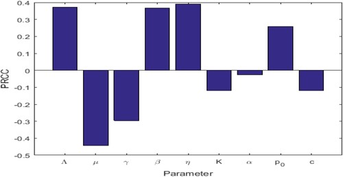
Table 3. Parameters scope and PRCC value corresponding to I.

Parameters	Range	PRCC	p-value
Λ	[ 0.00005,0.005]	0.3721	1.0273e−66
μ	[ 0,00006,0.005]	−0.3937	3.8870e−75
γ	[ 0,05,0.3]	−0.2752	4.3426e−36
β	[ 0,0001,0.01]	0.3926	1.0370e−74
η	[ 0.0001,0.01]	0.3917	2.4061e−74
K	[ 0.000008,0.001]	−0.1666	6.3926e−14
α	[ 0.00001,0.01]	−0.0453	0.0426
$P_0$	[ 0.00001,0.01]	0.2667	6.6169e−34
c	[ 0.00001,0.01]	−0.1265	1.3714e−08

The above PRCC analytical results indicated the dependence of the patients' number I on various parameters of the model [35, 43, 45]. From Table 3 and Figure 4, it can be seen that the influence of parameter Λ, β, η, $P_0$ on the number of patients I has a high sensitivity and positive correlation. Where $\begin{array}{rl}& \mathrm{\Lambda }(|PRCC|=0.3721),\text{β}(|PRCC|=0.3926),\\ & \eta (|PRCC|=0.3917),P_0(|PRCC|=0.2667)\end{array}$has the most significant positive impact on I. Therefore, if the recruitment rate of susceptible persons is higher, the conversion rate of susceptible persons becomes patients after inhaling PM${}_{2.5}$ is higher, and the greater the daily emission of PM${}_{2.5}$, then the number of patients will be higher.

In addition, the influence of parameters μ, γ, K, α, c on the number of patients are negatively correlated. Moreover, $\begin{array}{rl}& \mu (|PRCC|=0.3937),\gamma (|PRCC|=0.2752),\\ & K(|PRCC|=0.1666),c(|PRCC|=0.1265)\end{array}$has the most significant negative impact on I [26, 43, 45]. It can be seen that if the natural mortality rate of susceptible and infected people is higher, the cure rate of infected people is higher. The clearance rate for PM${}_{2.5}$ is higher, and the PM${}_{2.5}$ pathogenic threshold is higher, the number of patients will be lower. Although $\alpha (|PRCC|=0.0453)$ has a negative correlation with the number of patients I, its influence result is not significant within the hypothesis range of this paper.

4.2. Time-varying sensitivity analysis of parameters to the number of patients

Time-varying sensitivity refers to the influence of parameters on the output variable I as it changes over time. Therefore, time-varying sensitivity analysis can evaluate the incidence and dependence of a parameter variable in a dynamic model on the output variable over a period of time [38, 46].

Since the outbreak period and time quantum of different diseases are different, the influence of parameters on diseases also changes with time [38, 51]. Based on the pathogenetic process of respiratory diseases, time-varying sensitivity analysis of parameters to the number of patients is considered from two aspects, continuous time period and single point time, respectively.

4.2.1. Time-varying sensitivity analysis of parameters to the number of patients in a continuous period

This section mainly studies the time-varying sensitivity analysis of parameters to the number of patients within a continuous period of 0–50. The results are shown in Figure 5, where parameter is the input variable, and the number of patients is the output variable. The range of grey interval is [-0.05,0.05], indicating that the change of the parameter in this region has no significant impact on the patients' number I [38, 46, 51].

Figure 5. Time-varying sensitivity analysis of parameters to the number of patients I.

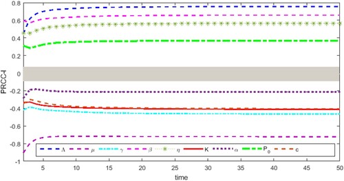
From Figure 5, it is found that the parameters change significantly in the early stage in the pathogenesis of respiratory diseases, especially before the time t = 10. With the change of time, the parameters μ, γ, K, α, c indicated negative correlation with the number of patients I, and maintained the negative effect. PM${}_{2.5}$ pathogenic threshold K has a large negative correlation, and the negative influence gradually increases and finally stabilizes. The clearance rate c for PM${}_{2.5}$ also has a large negative correlation with I, and its negative effect on I decreases first, then increases and finally becomes stable. The cure rate γ of infected persons has a great negative correlation, and its negative effect on I first slightly decreases, then presents a large increase and finally stabilizes. In addition, although there is also a large negative correlation between the natural mortality rate μ and the disease-induced mortality rate α of infected persons, it is ignored under the assumptions of this paper.

Furthermore, parameters Λ, β, η, $P_0$ proved positive correlation with the number of patients I, and maintained the positive effect. The recruitment rate Λ of susceptible persons has a significant positive correlation with I, and its positive effect increases significantly first and tends to be stable at last. The conversion rate β and the inhalation rate η for PM${}_{2.5}$ prove the significant positive correlation, and its positive influence on I decreases significantly first, then increasing and finally becomes stable. The daily emission $P_0$ of PM${}_{2.5}$ has a large positive correlation, and its positive impact on I decreases first, then increases and finally becomes stable.

Therefore, in order to effectively control the number of patients with respiratory diseases over a continuous period of time, the negative effects of clearance rate c for PM${}_{2.5}$ and the cure rate γ of infected persons on I should be mainly paid attention. Meanwhile, the positive effects of the conversion rate β of susceptible persons become patients after inhaling PM${}_{2.5}$, the inhalation rate η for PM${}_{2.5}$ and the daily emission $P_0$ of PM${}_{2.5}$ on I should be mainly paid attention.

4.2.2. Time-varying sensitivity analysis of parameters to the number of patients at a single point

From Figure 5, it is found that the incidence and dependence of different parameters on the number of patients I in a continuous period from 0 to 50. However, at a certain moment, different parameters have a different impact on the number of patients I. Therefore, the influence of parameters on state variables at a certain moment will be proposed in this section. The impact of parameters on the number of patients I at the time t = 10 is analysed as revealed in Figure 6–14. Where, the abscissa represents the residual of the linear regression between the sorted parameter and remaining parameters, the ordinate represents the residual of linear regression between the number of patients I after sorting and other parameters [38, 46, 51].

Figure 6. The PRCC scatter plot for η.

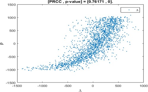
Figure 7. The PRCC scatter plot for η.

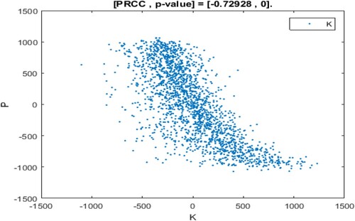
Figure 8. The PRCC scatter plot for η.

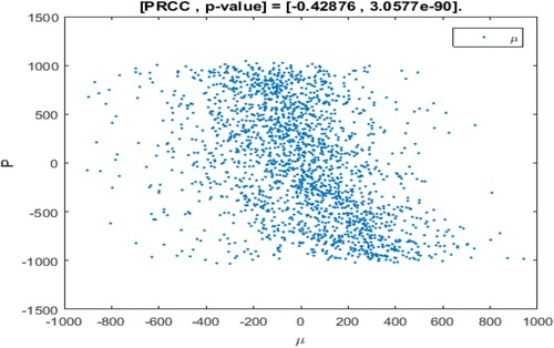
Figure 9. The PRCC scatter plot for η.

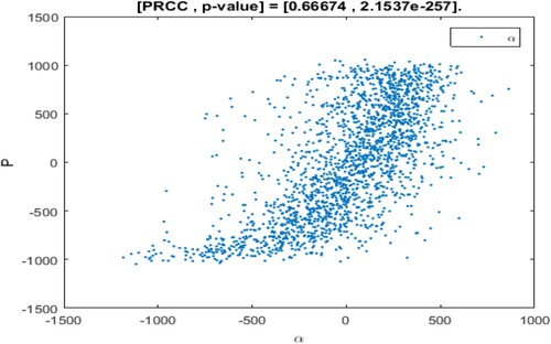
Figure 10. The PRCC scatter plot for η.

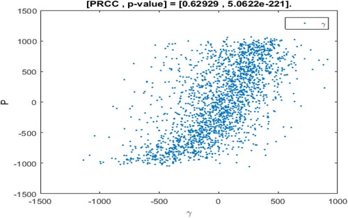
Figure 11. The PRCC scatter plot for η.

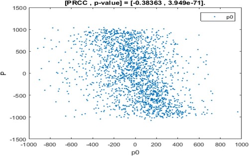
Figure 12. The PRCC scatter plot for η.

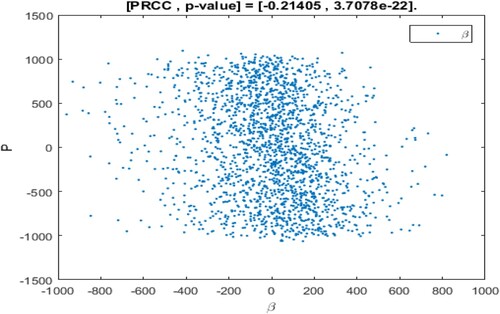
Figure 13. The PRCC scatter plot for η.

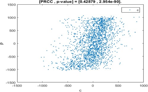
Figure 14. The PRCC scatter plot for η.

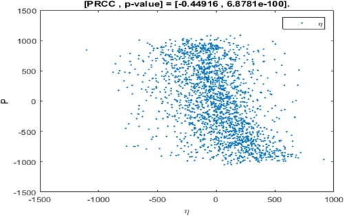
As shown in Figures 6–14, the monotony of parameters Λ, γ, α, K is the most significant at the time t = 10, that is, patients with respiratory diseases are mainly influenced by the changes of these parameters at this time. Where, parameters Λ, γ, α shows the monotonously increasing situation, that is, the recruitment rate of susceptible people, the cure rate of patients and the mortality rate of infected people have the positive impact on patients with respiratory diseases. The parameter K shows a monotonously decreasing situation, that is, the PM${}_{2.5}$ pathogenic threshold at this moment has a negative impact on the number of patients I. In addition, the parameters β, η, μ, $P_0$ present the relatively weak monotonously decreasing situation, and the parameter c presents a relatively weak monotonously increasing situation. This indicates that these parameters are not sensitive to the influence of patients with respiratory diseases at t = 10.

To sum up, the parameters have different sensitivities to the number of patients with respiratory diseases at t = 10. From Figures 6–14, it is found that parameters β, η, c, $P_0$ are insensitive to the number of patients at the time t = 10, that is, the conversion rate of susceptible individuals becomes patients by inhaling PM${}_{2.5}$, the inhalation rate for PM${}_{2.5}$, the clearance rate for PM${}_{2.5}$ and the daily emission $P_0$ of PM${}_{2.5}$ have no significant influence on the number of patients at that time. Therefore, we suggest that it is of great significance to control the outbreak and transmission of respiratory diseases by adjusting more sensitive parameters for a different number of patients at a certain time.

5. Optimal control

It is well known that the control of respiratory diseases by means of constant control can not achieve the desired effect. This is because of control parameters are time-dependent, and in order to achieve effective disease control within a limited time frame, time-related control strategies need to be considered [15, 48]. In this section, reducing conversion rate, increasing treatment rate and improving clearance rate are considered time-dependent controls over a limited time. It is striving to reduce the number of patients at the lowest possible control cost, and enable to decrease the PM${}_{2.5}$ emissions, and ultimately achieve the goal of controlling the outbreak and spread of respiratory diseases.

First of all, three control functions related to time are introduced into the model (1(1) $\{\begin{array}{l}{\displaystyle \frac{\mathrm{d}S}{\mathrm{d}t}}=\mathrm{\Lambda }-\mu S+\gamma I-{\displaystyle \frac{\text{β}\eta SP}{K+P}},\\ {\displaystyle \frac{\mathrm{d}I}{\mathrm{d}t}}={\displaystyle \frac{\text{β}\eta SP}{K+P}}-\mu I-\alpha I-\gamma I,\\ {\displaystyle \frac{\mathrm{d}P}{\mathrm{d}t}}=P_0-cP-\eta (S+I).\end{array}$(1) ), in which the control function $u_1\left(t\right)$ represented the enhanced treatment rate of patients. The specific implementation strategy is to identify the cause of the symptoms and go to a regular hospital for medical treatment. The control function $u_2\left(t\right)$ represents the reduced conversion rate of susceptible persons become patients by inhalation PM${}_{2.5}$. The specific measures are to strengthen physical exercise to improve their resistance, and wear masks to reduce the inhalation of susceptible people to PM${}_{2.5}$. The control function $u_3\left(t\right)$ represents the enhanced clearance rate for PM${}_{2.5}$. The specific implementation strategy is to develop strict industrial emission standards, increase the intensity of dust removal. The control function $u_1\left(t\right)$ is to promote the healing from the perspective of curing patients, the control function $u_2\left(t\right)$ is to decrease the transmission of respiratory diseases from the perspective of cutting off the transmission route, the control function $u_3\left(t\right)$ is to reduce the outbreak of respiratory diseases from the perspective of removing PM${}_{2.5}$. Finally, the model (1(1) $\{\begin{array}{l}{\displaystyle \frac{\mathrm{d}S}{\mathrm{d}t}}=\mathrm{\Lambda }-\mu S+\gamma I-{\displaystyle \frac{\text{β}\eta SP}{K+P}},\\ {\displaystyle \frac{\mathrm{d}I}{\mathrm{d}t}}={\displaystyle \frac{\text{β}\eta SP}{K+P}}-\mu I-\alpha I-\gamma I,\\ {\displaystyle \frac{\mathrm{d}P}{\mathrm{d}t}}=P_0-cP-\eta (S+I).\end{array}$(1) ) is transformed into the following form (3) $\{\begin{array}{l}{\displaystyle \frac{\mathrm{d}S}{\mathrm{d}t}}=\mathrm{\Lambda }-\mu S+\gamma (1+u_1\left(t\right))I-\text{β}(1-u_2\left(t\right)){\displaystyle \frac{\eta SP}{K+P}},\\ {\displaystyle \frac{\mathrm{d}I}{\mathrm{d}t}}=\text{β}(1-u_2\left(t\right)){\displaystyle \frac{\eta SP}{K+P}}-\mu I-\alpha I-\gamma (1+u_1\left(t\right))I,\\ {\displaystyle \frac{\mathrm{d}P}{\mathrm{d}t}}=P_0-c(1+u_3\left(t\right))P-\eta (S+I),\end{array}$(3) First, the objective function corresponding to model (3(3) $\{\begin{array}{l}{\displaystyle \frac{\mathrm{d}S}{\mathrm{d}t}}=\mathrm{\Lambda }-\mu S+\gamma (1+u_1\left(t\right))I-\text{β}(1-u_2\left(t\right)){\displaystyle \frac{\eta SP}{K+P}},\\ {\displaystyle \frac{\mathrm{d}I}{\mathrm{d}t}}=\text{β}(1-u_2\left(t\right)){\displaystyle \frac{\eta SP}{K+P}}-\mu I-\alpha I-\gamma (1+u_1\left(t\right))I,\\ {\displaystyle \frac{\mathrm{d}P}{\mathrm{d}t}}=P_0-c(1+u_3\left(t\right))P-\eta (S+I),\end{array}$(3) ) is proposed as follows (4) $\begin{array}{rl}& J\left(u_1\right(t),u_2(t),u_3(t\left)\right)\\ & =\underset{u_1,u_2,u_3}{min}{\int }_0^{t_f}[a_{1}I\left(t\right)+a_{2}P\left(t\right)+b{u_1}^2\left(t\right)+c_1{u_2}^2\left(t\right)+d{u_3}^2\left(t\right)]\mathrm{d}t\end{array}$(4) where $a_1,a_2(0<a_1,a_2<1)$, b, $c_1$, d are positive weighting coefficient, $a_{1}I\left(t\right)$ represents the number of infected persons, $a_{2}P\left(t\right)$ is the concentration of PM${}_{2.5}$. The item $b{u_1}^2$, $c_1{u_2}^2$ and $d{u_3}^2$ represent the cost corresponding to the cure control, conversion control and clearance control, respectively. Here, the control variable is squared to eliminate side effects [15, 30]. For the objective function $J\left(u_1\right(t),u_2(t),u_3(t\left)\right)$, the optimal control function $\left({u_1}^{\ast }\right(t),{u_2}^{\ast }(t),{u_3}^{\ast }(t\left)\right)$ needs to be sought to make the objective function reach the minimum value, that is, to minimize the total cost of controlling the outbreak and spread of respiratory diseases and reducing the emission of PM${}_{2.5}$, that is, (5) $J({u_1}^{\ast }\left(t\right),{u_2}^{\ast }\left(t\right),{u_3}^{\ast }\left(t\right))=min\{J(u_1\left(t\right),u_2\left(t\right),u_3\left(t\right)):(u_1\left(t\right),u_2\left(t\right),u_3\left(t\right))\in \varphi \}$(5) here, $\varphi =\left\{u_i\right(t):0\le u_i(t)\le 1,i=1,2,3;0\le t\le t_f,u_i(t\left)\mathrm{i}\mathrm{s}\mathrm{L}\mathrm{e}\mathrm{b}\mathrm{e}\mathrm{s}\mathrm{g}\mathrm{u}\mathrm{e}\mathrm{m}\mathrm{e}\mathrm{a}\mathrm{s}\mathrm{u}\mathrm{r}\mathrm{a}\mathrm{b}\mathrm{l}\mathrm{e}\right\}$.

To obtain the optimal solution, let us define the following Lagrangian function (6) $L(I,P,u_i)=a_{1}I\left(t\right)+a_{2}P\left(t\right)+b{u_1}^2\left(t\right)+c_1{u_2}^2\left(t\right)+d{u_3}^2\left(t\right).$(6) Then, the Pontryagin's Maximal Principle is applied to determine the conditions under which effective control of respiratory diseases can be achieved in a limited time. This principle transforms the Equations (3(3) $\{\begin{array}{l}{\displaystyle \frac{\mathrm{d}S}{\mathrm{d}t}}=\mathrm{\Lambda }-\mu S+\gamma (1+u_1\left(t\right))I-\text{β}(1-u_2\left(t\right)){\displaystyle \frac{\eta SP}{K+P}},\\ {\displaystyle \frac{\mathrm{d}I}{\mathrm{d}t}}=\text{β}(1-u_2\left(t\right)){\displaystyle \frac{\eta SP}{K+P}}-\mu I-\alpha I-\gamma (1+u_1\left(t\right))I,\\ {\displaystyle \frac{\mathrm{d}P}{\mathrm{d}t}}=P_0-c(1+u_3\left(t\right))P-\eta (S+I),\end{array}$(3) ), (4(4) $\begin{array}{rl}& J\left(u_1\right(t),u_2(t),u_3(t\left)\right)\\ & =\underset{u_1,u_2,u_3}{min}{\int }_0^{t_f}[a_{1}I\left(t\right)+a_{2}P\left(t\right)+b{u_1}^2\left(t\right)+c_1{u_2}^2\left(t\right)+d{u_3}^2\left(t\right)]\mathrm{d}t\end{array}$(4) ), (5(5) $J({u_1}^{\ast }\left(t\right),{u_2}^{\ast }\left(t\right),{u_3}^{\ast }\left(t\right))=min\{J(u_1\left(t\right),u_2\left(t\right),u_3\left(t\right)):(u_1\left(t\right),u_2\left(t\right),u_3\left(t\right))\in \varphi \}$(5) ), and (6(6) $L(I,P,u_i)=a_{1}I\left(t\right)+a_{2}P\left(t\right)+b{u_1}^2\left(t\right)+c_1{u_2}^2\left(t\right)+d{u_3}^2\left(t\right).$(6) ) into Hamiltonian point-state minimization of the control function $u_1\left(t\right)$, $u_2\left(t\right)$, $u_3\left(t\right)$ [8, 30].

Hence, the Hamiltonian function is defined as follows (7) $\begin{array}{rl}H(t,X,U,\lambda )& =L+{\lambda }_1\left(t\right)\frac{\mathrm{d}S}{\mathrm{d}t}+{\lambda }_2\left(t\right)\frac{\mathrm{d}I}{\mathrm{d}t}+{\lambda }_3\left(t\right)\frac{\mathrm{d}P}{\mathrm{d}t}\\ & =a_{1}I\left(t\right)+a_{2}P\left(t\right)+b{u_1}^2\left(t\right)+c_1{u_2}^2\left(t\right)+d{u_3}^2\left(t\right)\\ & +{\lambda }_1\left(t\right)\{\mathrm{\Lambda }-\mu S+\gamma (1+u_1\left(t\right))I-\text{β}(1-u_2\left(t\right)\left)\frac{\eta SP}{K+P}\right\}\\ & +{\lambda }_2\left(t\right)\left\{\text{β}\right(1-u_2\left(t\right))\frac{\eta SP}{K+P}-\mu I-\alpha I-\gamma (1+u_1\left(t\right)\left)I\right\}\\ & +{\lambda }_3\left(t\right)\{P_0-c(1+u_3\left(t\right))P-\eta (S+I)\}.\end{array}$(7) Where, $X\left(t\right)=\left(S\right(t),I(t),P(t\left)\right)$, $U\left(t\right)=\left(u_1\right(t),u_2(t),u_3(t\left)\right)$, ${\lambda }_i\left(t\right)(i=1,2,3)$ is the adjoint variable.

Theorem 5.1

Assume that $\left(X^{\ast }\right(t),U^{\ast }(t\left)\right)$ is the optimal solution of the corresponding control system, there exists a vector function $\lambda \left(t\right)=\left({\lambda }_1\right(t),{\lambda }_2(t),{\lambda }_3(t\left)\right)$ that satisfies the following equation (8) $\{\begin{array}{l}{\dot{\lambda }}_1\left(t\right)=\mu {\lambda }_1\left(t\right)+({\lambda }_1\left(t\right)-{\lambda }_2\left(t\right))\left[\text{β}(1-u_2\left(t\right)){\displaystyle \frac{\eta \overline{P}}{K+\overline{P}}}\right]+{\lambda }_3\left(t\right)\eta ,\\ {\dot{\lambda }}_2\left(t\right)=-a_1+({\lambda }_2\left(t\right)-{\lambda }_1\left(t\right))\left[\gamma (1+u_1\left(t\right))\right]+{\lambda }_2\left(t\right)(\mu +\alpha )+{\lambda }_3\left(t\right)\eta ,\\ {\dot{\lambda }}_3\left(t\right)=-a_2+({\lambda }_1\left(t\right)-{\lambda }_2\left(t\right))\text{β}(1-u_2\left(t\right)){\displaystyle \frac{\eta \overline{S}K}{{(K+\overline{P})}^2}}+{\lambda }_3\left(t\right)c(1+u_3\left(t\right)),\end{array}$(8) and it has a transversality condition (9) ${\lambda }_i\left(t_f\right)=0,i=1,2,3.$(9) Moreover, the optimal control function is given (10) $\{\begin{array}{rl}{u_1}^{\ast }\left(t\right)& =max\{0,min(1,{\tilde{u}}_1)\},\\ {u_2}^{\ast }\left(t\right)& =max\{0,min(1,{\tilde{u}}_2)\},\\ {u_3}^{\ast }\left(t\right)& =max\{0,min(1,{\tilde{u}}_3)\},\end{array}$(10) where ${\tilde{u}}_1=\frac{\gamma ({\overline{\lambda }}_2-{\overline{\lambda }}_1)\overline{I}}{2b}$, ${\tilde{u}}_2=\frac{({\overline{\lambda }}_2-{\overline{\lambda }}_1)\text{β}\eta \overline{S}\overline{P}}{2c_1(K+\overline{P})}$, ${\tilde{u}}_3=\frac{c\overline{P}{\lambda }_3}{2d}$.

Proof.

According to the Pontryagin's Maximum Principle and the existence of the optimal control pair [8, 37], the following conclusions can be found that (11) $\{\begin{array}{ll}{\displaystyle \frac{\mathrm{\partial }H(t,X,U,\lambda )}{\mathrm{\partial }U}}=0,& \left(\mathrm{o}\mathrm{p}\mathrm{t}\mathrm{i}\mathrm{m}\mathrm{a}\mathrm{l}\mathrm{i}\mathrm{t}\mathrm{y}\mathrm{c}\mathrm{o}\mathrm{n}\mathrm{d}\mathrm{i}\mathrm{t}\mathrm{i}\mathrm{o}\mathrm{n}\right)\\ {\lambda }^{\mathrm{\prime }}={\displaystyle \frac{\mathrm{\partial }H(t,X,U,\lambda )}{\mathrm{\partial }U}},& \left(\mathrm{a}\mathrm{d}\mathrm{j}\mathrm{o}\mathrm{i}\mathrm{n}\mathrm{t}\mathrm{c}\mathrm{o}\mathrm{n}\mathrm{d}\mathrm{i}\mathrm{t}\mathrm{i}\mathrm{o}\mathrm{n}\right)\\ \lambda \left(t_f\right)=0,& \left(\mathrm{t}\mathrm{r}\mathrm{a}\mathrm{n}\mathrm{s}\mathrm{v}\mathrm{e}\mathrm{r}\mathrm{s}\mathrm{a}\mathrm{l}\mathrm{i}\mathrm{t}\mathrm{y}\mathrm{c}\mathrm{o}\mathrm{n}\mathrm{d}\mathrm{i}\mathrm{t}\mathrm{i}\mathrm{o}\mathrm{n}\right)\end{array}$(11) Then, according to the adjoint condition, the partial derivative of the Hamiltonian function for the associated state equation with $X=X^{\ast }$ is calculated, and one has (12) $\{\begin{array}{rl}{\dot{\lambda }}_1\left(t\right)& ={\displaystyle \frac{\mathrm{\partial }H(t,X,U,\lambda )}{\mathrm{\partial }S}},\\ {\dot{\lambda }}_2\left(t\right)& ={\displaystyle \frac{\mathrm{\partial }H(t,X,U,\lambda )}{\mathrm{\partial }I}},\\ {\dot{\lambda }}_3\left(t\right)& ={\displaystyle \frac{\mathrm{\partial }H(t,X,U,\lambda )}{\mathrm{\partial }P}},\end{array}$(12) To minimize the Hamiltonian function under optimal control, and the function $H(t,X,U,\lambda )$ is differentiated on ϕ with respect to $u_1$, $u_2$, $u_3$, and is equivalent to zero. Then, the following solutions are proved: $\begin{array}{rl}& \frac{\mathrm{\partial }H(t,X,U,\lambda )}{\mathrm{\partial }{u}_1}=0\mathrm{g}\mathrm{e}\mathrm{t}\mathrm{s}{\tilde{u}}_1=\frac{\gamma ({\overline{\lambda }}_2-{\overline{\lambda }}_1)\overline{I}}{2b},\\ & \frac{\mathrm{\partial }H(t,X,U,\lambda )}{\mathrm{\partial }{u}_2}=0\mathrm{a}\mathrm{c}\mathrm{q}\mathrm{u}\mathrm{i}\mathrm{r}\mathrm{e}\mathrm{s}{\tilde{u}}_2=\frac{({\overline{\lambda }}_2-{\overline{\lambda }}_1)\text{β}\eta \overline{S}\overline{P}}{2c_1(K+\overline{P})},\\ & \frac{\mathrm{\partial }H(t,X,U,\lambda )}{\mathrm{\partial }{u}_3}=0\mathrm{g}\mathrm{a}\mathrm{i}\mathrm{n}\mathrm{s}{\tilde{u}}_3=\frac{c\overline{P}{\lambda }_3}{2d}.\end{array}$Where $\overline{S}$, $\overline{I}$, $\overline{P}$ are the optimal solutions corresponding to S, I, P, respectively, and $\{{\overline{\lambda }}_1,{\overline{\lambda }}_2,{\overline{\lambda }}_3\}$ is the solution of system (12(12) $\{\begin{array}{rl}{\dot{\lambda }}_1\left(t\right)& ={\displaystyle \frac{\mathrm{\partial }H(t,X,U,\lambda )}{\mathrm{\partial }S}},\\ {\dot{\lambda }}_2\left(t\right)& ={\displaystyle \frac{\mathrm{\partial }H(t,X,U,\lambda )}{\mathrm{\partial }I}},\\ {\dot{\lambda }}_3\left(t\right)& ={\displaystyle \frac{\mathrm{\partial }H(t,X,U,\lambda )}{\mathrm{\partial }P}},\end{array}$(12) ).

Then, according to the standard control parameters about control bounds, it can be obtained by calculation $\{\begin{array}{ll}0,& {\displaystyle \frac{\gamma ({\overline{\lambda }}_2-{\overline{\lambda }}_1)\overline{I}}{2b}}\le 0,\\ {\displaystyle \frac{\gamma ({\overline{\lambda }}_2-{\overline{\lambda }}_1)\overline{I}}{2b}},& 0<{\displaystyle \frac{\gamma ({\overline{\lambda }}_2-{\overline{\lambda }}_1)\overline{I}}{2b}}<1,\\ 1,& {\displaystyle \frac{\gamma ({\overline{\lambda }}_2-{\overline{\lambda }}_1)\overline{I}}{2b}}\le 1\end{array}$its compact form can be expressed as ${u_1}^{\ast }=max\{0,min(1,\frac{\gamma ({\overline{\lambda }}_2-{\overline{\lambda }}_1)\overline{I}}{2b}\left)\right\}$.

Similarly, the compact forms of ${u_2}^{\ast }$ and ${u_3}^{\ast }$ can be, respectively, expressed as $\begin{array}{rl}{u_2}^{\ast }& =max\{0,min(1,\frac{({\overline{\lambda }}_2-{\overline{\lambda }}_1)\text{β}\eta \overline{S}\overline{P}}{2c_1(K+\overline{P})})\},\\ {u_3}^{\ast }& =max\{0,min(1,\frac{c\overline{P}{\lambda }_3}{2d})\}.\text{■}\end{array}$

6. Numerical simulation

In this section, we conduct numerical simulation of the optimal control of respiratory diseases. The parameters are selected in the following Table 4. The weight in the objective function is $a_1=0.8$, $a_2=0.5$, b = 0.2, $c=0.006$, d = 1000.

Tab. 4. Parameter values in simulation.

Parameter	Definition	Value	Reference
$\mathrm{\Lambda }$	the recruitment rate of susceptible persons	0.05	[13,14,39,40]
$\mu$	the natural mortality rate of susceptible and infected persons	0.01428	[13,14,39,40]
$\alpha$	the disease-induced mortality rate of infected persons	0.02	[13,14,39,40]
$\text{β}$	the conversion rate of susceptible individuals become patients by inhaling PM2.5	0.002	[13,14,39,40]
$\eta$	the inhalation rate for PM2.5 per person	0.01	Estimated
$\gamma$	the cure rate of infected persons	0.04	[13,14,39,40]
$K$	the PM2.5 pathogenic threshold	100	[25,26,27]
$P_0$	the daily emissions of PM2.5	190	[28,29,30]
$c$	the clearance rate for PM2.5	0.9	Estimated

From Figure 15, it is illustrated that the effectiveness of the optimal control. Respiratory diseases will break out very quickly in a very short period if no control strategies are implemented. Under the optimal control strategy, the prevalence of respiratory diseases declined rapidly and remained at a very low level.

Figure 15. Prevalence of respiratory diseases under optimal control strategies.

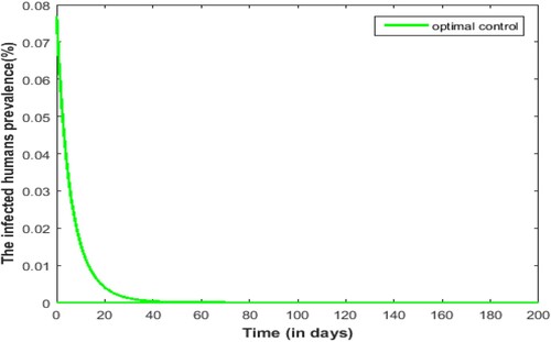
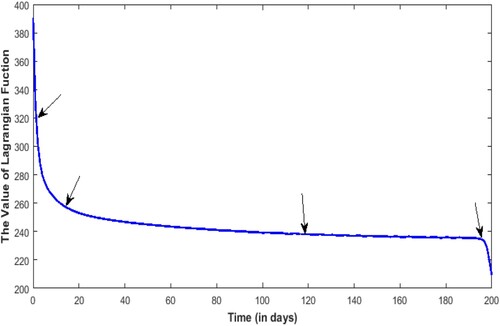
Figure 16 illustrates how the control strategy changes over time. In the whole pathogenesis process of respiratory diseases, improving the cure rate, reducing the conversion rate and improving the clearance rate are very helpful to reduce the incidence of respiratory diseases. As can be seen from Figure 17, in the early stage, with the reduction of the Lagrangian function, the clearance rate of PM${}_{2.5}$ began to decrease. Around the fifth day, the treatment rate for the patients began to decrease dramatically as the Lagrangian function decreased sharply. At about day 18, the conversion rate began to slow down as the Lagrangian function decreased. In the final stage of about 195 days, as the Lagrangian function rapidly reaches its minimum, the clearance rate of PM${}_{2.5}$ and the conversion rate also decrease rapidly. Finally, all the control strategy functions return to 0 when the transversal condition is ${\lambda }_i\left(t_f\right)=0$. Also, the arrows in Figure 16 and 17 are paired at each turning point.

Figure 16. Diagram of control strategy $u_1$, $u_2$, $u_3$ over time. Control strategies of strengthening the treatment of patients (red line); Control strategies to reduce conversion of susceptible persons to patients (blue line); Control strategies of enhancing removal for PM${}_{2.5}$ (green line).

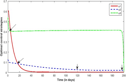
Figure 17. Lagrangian functions with time-varying optimal control.

By comparing Figure 16 and 17, it can be seen that with regard to the reduction of the cost function, in the short term, the control of the treatment of patients and the conversion control of susceptible people becomes patients are more effective than the control of PM${}_{2.5}$ clearance. From the long-term perspective of the control of respiratory diseases, the control strategy for PM${}_{2.5}$ removal should always be unremitting.

7. Conclusion and discussion

Under normal circumstances, polluted air contains a large amount of fine particulate matter (PM${}_{2.5}$). After PM${}_{2.5}$ is inhaled by susceptible people exposed to polluted air, the human respiratory system will be damaged and various respiratory diseases will be caused. In this paper, the actual situation that the susceptible population directly fell ill after inhaling PM${}_{2.5}$ is taken into account. The SISP respiratory disease model is built by introducing the PM${}_{2.5}$ pathogenic threshold, and adding a differential equation describing the dynamic change of PM${}_{2.5}$. The influence of daily emission of PM${}_{2.5}$ and PM${}_{2.5}$ pathogenic threshold on the incidence and spread of respiratory diseases are studied, so as to provide an optimal control strategy for the outbreak and spread of respiratory diseases.

According to the existence analysis of the equilibrium in Table 1, it can be seen that the system (1(1) $\{\begin{array}{l}{\displaystyle \frac{\mathrm{d}S}{\mathrm{d}t}}=\mathrm{\Lambda }-\mu S+\gamma I-{\displaystyle \frac{\text{β}\eta SP}{K+P}},\\ {\displaystyle \frac{\mathrm{d}I}{\mathrm{d}t}}={\displaystyle \frac{\text{β}\eta SP}{K+P}}-\mu I-\alpha I-\gamma I,\\ {\displaystyle \frac{\mathrm{d}P}{\mathrm{d}t}}=P_0-cP-\eta (S+I).\end{array}$(1) ) has a disease-free equilibrium $E_0$ if the daily emission $P_0$ of PM${}_{2.5}$ is a constant. Obviously, this is unrealistic, because PM${}_{2.5}$ has many emission sources, and the new emissions change every day. There are two endemic equilibria $E_2^{\ast }$ and $E_3^{\ast }$ in the system when the daily emission $P_0$ of PM${}_{2.5}$ is less than $\eta \frac{\mathrm{\Lambda }}{\mu }$ and the PM${}_{2.5}$ pathogenic threshold is between $K_5$ and $K_1$. These two endemic equilibria will degenerate into one endemic equilibrium $E_1^{\ast }$, and once the pathogenic threshold is $K_1$. The system only has an endemic equilibrium $E_2^{\ast }$ when the emission $P_0$ of PM${}_{2.5}$ is between $\eta \frac{\mathrm{\Lambda }}{\mu }$ and $\eta \frac{\mathrm{\Lambda }}{\mu }(1+\frac{\alpha }{\mu +\alpha })$. From the above analysis, it can be seen that the daily emission $P_0$ of PM${}_{2.5}$ and the size of PM${}_{2.5}$ pathogenic threshold have the great influence on the existence of the equilibria. In system (1(1) $\{\begin{array}{l}{\displaystyle \frac{\mathrm{d}S}{\mathrm{d}t}}=\mathrm{\Lambda }-\mu S+\gamma I-{\displaystyle \frac{\text{β}\eta SP}{K+P}},\\ {\displaystyle \frac{\mathrm{d}I}{\mathrm{d}t}}={\displaystyle \frac{\text{β}\eta SP}{K+P}}-\mu I-\alpha I-\gamma I,\\ {\displaystyle \frac{\mathrm{d}P}{\mathrm{d}t}}=P_0-cP-\eta (S+I).\end{array}$(1) ), the existence of disease-free equilibrium is only an ideal state, while the existence of endemic equilibrium is the normal state. Therefore, the long-term exposure of the susceptible population in the air environment of excessive PM${}_{2.5}$ emissions will easily induce the outbreak of respiratory diseases.

From the analysis results of the local and global stability of the system equilibrium in Table 2, on the premise that the existence condition of the system equilibrium is true, it is found that the disease-free equilibrium $E_0$ is locally asymptotically stable if the PM${}_{2.5}$ pathogenic threshold K is greater than $\frac{\text{β}{\eta }^2\mathrm{\Lambda }\alpha }{c{\mu }^2(\mu +\alpha +\gamma )}$. The globally asymptotically stable occurs when K is greater than $\frac{\text{β}\eta \mathrm{\Lambda }}{c\mu }$. When the daily emission $P_0$ of PM${}_{2.5}$ is greater than $\overline{P}$ and PM${}_{2.5}$ pathogenic threshold K is greater than $\overline{K}$, the endemic equilibria $E_2^{\ast }$ and $E_3^{\ast }$ are locally asymptotically stable. The global asymptotic stability occurs when $P_0$ is greater than $\frac{\mathrm{\Lambda }c(2\mu +\alpha )}{\mu (\mu +\alpha )K}$. When the daily emission $P_0$ of PM${}_{2.5}$ is greater than $\overline{P}$ and PM${}_{2.5}$ pathogenic threshold K is $K_1=\overline{K}$, the endemic equilibrium $E_1^{\ast }$ is locally asymptotically stable. The global asymptotic stability occurs when the daily emission $P_0$ of PM${}_{2.5}$ is greater than $\frac{\mathrm{\Lambda }c(2\mu +\alpha )}{\mu (\mu +\alpha )K_1}$. When the daily emission $P_0$ of PM${}_{2.5}$ is less than $\tilde{P}$ and PM${}_{2.5}$ pathogenic threshold K is greater than $\tilde{K}$, the endemic equilibrium $E_2^{\ast }$ is locally asymptotically stable. The global asymptotically stable occurs when $P_0$ is less than $\hat{P}$ and K is greater than $\hat{K}$. It is easy to know from the theoretical analysis that the daily emission $P_0$ of PM${}_{2.5}$ and PM${}_{2.5}$ pathogenic threshold K have the strong influence on the stability of equilibrium. Where, the equilibrium can reach local or global asymptotic stability only if the daily emission $P_0$ of PM${}_{2.5}$ is within a certain range. The higher the PM${}_{2.5}$ pathogenic threshold K is, the easier it is for the endemic equilibrium to reach stability, which is not conducive to the control of respiratory diseases.

According to the above sensitivity theoretical analysis, it can be seen that the influence of parameters Λ, β, η, $p_0$ on the number of patients I have the high sensitivity and positive correlation. The influence of parameters μ, γ, K, α, c on the number of patients I are negatively correlation. That is to say, the greater the recruitment rate of susceptible people, the greater the conversion rate of susceptible people becomes patients after inhaling PM${}_{2.5}$, the greater the PM${}_{2.5}$ inhalation rate, and the greater the daily emission $P_0$ of PM${}_{2.5}$, the more patients will be. The greater the natural mortality rate of susceptible and infected people, the greater the cure rate of infected people, the greater the clearance rate for PM${}_{2.5}$, and the greater the PM${}_{2.5}$ pathogenic threshold, the littler the number of patients will be.

On the basis of the optimal control analysis, for human respiratory diseases caused by air pollution, the first step is to improve the PM${}_{2.5}$ clearance rate, and the specific control strategy is to reduce the daily emission $P_0$ of PM${}_{2.5}$ and increase the intensity of dust removal, etc. Next, improve the cure rate, and the specific control strategy is to treat the patients in time. Then, to reduce the conversion rate of susceptible people becomes patients, and the specific control strategy is to remind people to wear masks in severe air pollution weather, as far as possible to avoid going out and so on. It is worth noting that the removal of PM${}_{2.5}$ is a long and difficult work that needs to be sustained for a long time.

Disclosure statement

The authors declare that they have no known competing financial interests or personal relationships that could have appeared to influence the work reported in this paper.

Additional information

Funding

This research is supported by the National Natural Science Foundation of China [grant number 11401002], the Natural Science Foundation of Anhui Province [grant number 2008085MA02], the Natural Science Foundation for Colleges and Universities in Anhui Province [grant number KJ2018A0029], the Teaching Research Project of Anhui University [grant number ZLTS2016065], the Quality engineering project of colleges and universities in Anhui Province [grant number 2020jyxm0103] and the Science Foundation of Anhui Province Universities [grant number KJ2019A005].

References

- C.J. Browne, X. Pan, H. Shu, and X.S. Wang, Resonance of periodic combination antiviral therapy and intracellular delays in virus model, Bullet. Math. Biol. 82(2) (2020), pp. 1–29.
- S. Cai, Q. Ma, and S. Wang, Impact of air pollution control policies on future PM2.5 concentrations and their source contributions in China, J. Environ. Manag. 227 (2018), pp. 124–133.
- Y. Cai, S. Zhao, Y. Niu, Z. Peng, K. Wang, D. He, and W. Wang, Modelling the effects of the contaminated environments on tuberculosis in Jiangsu, China, J. Theor. Biol. 508 (2020), pp. 110453.
- D. Chen, Y. Xiao, and S. Tang, Air quality index induced nonsmooth system for respiratory infection, J. Theoret. Biol. 460 (2018), pp. 160–169.
- P.H. Chowdhury, H. Okano, A. Honda, H. Kudou, G. Kitamura, S. Ito, K. Ueda, and H. Takano, Aqueous and organic extract of PM2.5 collected in different seasons and cities of Japan differently affect respiratory and immune systems, Environmental Pollution 235 (2017), pp. 223–234.
- C.T. Codeco, Endemic and epidemic dynamics of cholera: The role of the aquatic reservoir, BMC Infectious Diseases 1(1) (2001), pp. 1.
- M. Cohen, A.J. Brauer, R. Burnett, H.R. Anderson, J. Frostad, K. Estep, K. Balakrishnan, B. Brunekreef, L. Dandona, R. Dandona, and V. Feigin, Estimates and 25-year trends of the global burden of disease attributable to ambient air pollution: An analysis of data from the global burden of diseases study 2015, Lancet. 389(10082) (2018), pp. 1907–1918.
- C. Ding, Z. Qiu, and H. Zhu, Multi-host transmission dynamics of schistosomiasis and its optimal control, Math. Biosci. Eng. 12(5) (2015), pp. 983–1006.
- J. Dong, Y. Wang, J. Wang, and H. Bao, Association between atmospheric PM2.5 and daily outpatient visits for children's respiratory diseases in Lanzhou, Int. J. Biometeorol. 2021(3) (2021), pp. 1–11.
- G.B. Hamra, N. Guha, A. Cohen, F. Laden, O. Raaschou-Nielsen,, J.M. Samet,, P. Vineis, F. Forastiere, P. Saldiva, T. Yorifuji, and D. Loomis, Outdoor particulate matter exposure and lung cancer: A systematic review and meta-analysis, Environmental Health Perspectives 122(9) (2014), pp. 906–911.
- S. He, S. Tang, Y. Xiao, and R.A. Cheke, Stochastic modelling of air pollution impacts on respiratory infection risk, Bullet. Math. Biol. 80 (2018), pp. 3127–3153.
- P.K. Hopke, D. Croft, W. Zhang, S. Lin, M. Masiol, S. Squizzato, S.W. Thurston, E. van Wijngaarden, M.J. Utell, and D.Q. Rich, Changes in the acute response of respiratory diseases to PM2.5 in New York state from 2005 to 2016, Science of The Total Environment 677 (2019), pp. 328–339.
- H.F. Huo, R. Chen, and X.Y. Wang, Modelling and stability of HIV/AIDS epidemic model with treatment, Appl. Math. Model. 40(13–14) (2016), pp. 6550–6559.
- Institute for Health Metrics and Evaluation(IHME), GBD 2017, ambient particulate matter pollution, both sexes, all ages, 2017, deaths/DALYs [EB/OL], (2020-02-07) [2020-03016], Available at https://vizhub.healthdata.org/gbd-compare/.
- R. Jan and Y. Xiao, Effect of partial immunity on transmission dynamics of dengue disease with optimal control, Math. Meth. Appl. Sci. 42 (2019), pp. 1967–1983.
- S. Jing, H. Huo, and H. Xiang, Modeling the effects of meteorological factors and unreported cases on seasonal influenza outbreaks in Gansu Province, China, Bullet. Math. Biol. 82(6) (2020), pp. 73.
- R.I. Joh, W. Hao, H. Weiss, and J.S. Weitz, Dynamics of indirectly transmitted infectious diseases with immunological threshold, Bullet. Math. Biol. 71(4) (2008), pp. 845–862.
- A. Kumar, P.K. Srivastava, and R.P. Gupta, Nonlinear dynamics of infectious diseases via information-induced vaccination and saturated treatment – Science Direct, Math. Comput. Simul. 157 (2019), pp. 77–99.
- J.D. Kong, W. Davis, and W. Hao, Dynamics of a cholera transmission model with immunological threshold and natural phage control in reservoir, Bullet. Math. Biol. 76(8) (2014), pp. 2025–2051.
- J.D. Kong, W. Davis, X. Li, and H. Wang, Stability and sensitivity analysis of the iSIR model for indirectly transmitted infectious diseases with immunological threshold, SIAM J. Appl. Math. 74(5) (2014), pp. 1418–1441.
- J. Li, Z. Teng, G. Wang, L. Zhang, and C. Hu, Stability and bifurcation analysis of an SIR epidemic model with logistic growth and saturated treatment, Chaos, Solitons and Fractals: Appl. Sci. Eng.: An Interdisciplinary J. Nonlinear Sci. 99 (2017), pp. 63–71.
- Y. Liao, J. Sun, Z. Qian, S. Mei, Y. Li, Y. Lu, S.E. McMillin, H. Lin, and L. Lang, Modification by seasonal influenza and season on the association between ambient air pollution and child respiratory diseases in Shenzhen, China, Atmospheric Environment 234 (2020), pp. 117621.
- S Lim, T Vos, and A Flaxman, A comparative risk assessment of burden of disease and injury attributable to 67 risk factors and risk factor clusters in 21 regions, 1990-2010: A systematic analysis for the global burden of disease study 2010, Lancet 380(9859) (2012), pp. 2224–2260.
- Y. Liu and C.K. Ao, Effect of air pollution on health care expenditure: Evidence from respiratory diseases, Health Economics 30(4) (2021), pp. 858–875.
- M. Lu, J. Huang, S. Ruan, and P. Yu, Global dynamics of a susceptible-infectious-recovered epidemic model with a generalized non-monotone incidence rate, J. Dyn. Differ. Equ. 3 (2020), pp. 1–37.
- S. Marino, I.B. Hogue, C.J. Ray, and D.E. Kirschner, A methodology for performing global uncertainty and sensitivity analysis in systems biology, J. Theor. Biol. 254(1) (2009), pp. 178–196.
- Ministry of Environmental Protection, Air quality and quantity of heavy point area and 74 cities in 20 and 13 years[EB, OL] (2014-03-25) [2016-05-26], Available at http://www.zhb.gov.cn/gkml/hbb//t20140325269648.htm.
- M. Pascual, M.J. Bouma, and A.P. Dobson, Cholera and climate: Revisiting the quantitative evidence, Microbes and Infection 4(2) (2002), pp. 237–245.
- D.Y.H. Pui, S.C. Chen, and Z. Zuo, PM 2.5 in China: measurements, sources, visibility and health effects, and mitigation, Particuology 13(1) (2014), pp. 1–26.
- L. Qi, M. Xue, J. Cui, Q. Wang, and T. Wang, Schistosomiasis transmission model and its control in Anhui province, Bullet. Math. Biol. 80 (2018), pp. 2435–2451.
- D.E. Schraufnagel, Global alliance against chronic respiratory diseases symposium on air pollution: Overview and highlights, Chinese Med. J. 133(13) (2020), pp. 1–6.
- H.A. Shahriyari, Y Nikmanesh, S Jalali, N. Tahery, A. Zhiani Fard, N. Hatamzadeh, K. Zarea, M. Cheraghi,, and M.J. Mohammadi, Air pollution and human health risks: Mechanisms and clinical manifestations of cardiovascular and respiratory diseases, Toxin Reviews 2021(12) (2021), pp. 1–12.
- L. Shi, X. Feng, L. Qi, Y. Xu, and S. Zhai, Modeling and predicting the influence of PM on children's respiratory diseases, Int. J. Bifurc. Chaos. 30(15) (2020), pp. 2050235.
- P. Song and Y. Xiao, Analysis of an epidemic system with two response delays in media impact function, Bullet. Math. Biol. 81 (2019), pp. 1582–1612.
- S. Tang, Y. Xiao, L. Yuan, R.A. Cheke, and J. Wu, Campus quarantine (Fengxiao) for curbing emergent infectious diseases: Lessons from mitigating A/H1N1 in Xi'an, China, J. Theor. Biol. 295(295) (2012), pp. 47–58.
- S. Tang, Q. Yan, W. Shi, X. Wang, X. Sun,, P. Yu,, J. Wu, and Y. Xiao, Measuring the impact of air pollution on respiratory infection risk in China, Environmental Pollution 232(2018) (2018), pp. 477–486.
- X. Wang, H. Peng, B. Shi, D. Jiang, S. Zhang, and B. Chen, Optimal vaccination strategy of a constrained time-varying SEIR epidemic model-Science direct, Commun. Nonlinear Sci. Numer. Simul. 67 (2019), pp. 37–48.
- X. Wang, S. Tang, J. Wu, Y. Xiao, and R.A. Cheke, A combination of climatic conditions determines major within-season dengue outbreaks in Guangdong Province, China, Parasites and Vectors 12(1) (2019), pp. 1–10.
- J. Wang, Y. Xiao, and R.A. Cheke, Modelling the effects of contaminated environments on HFMD infections in mainland China, Biosystems 140 (2016), pp. 1–7.
- World Health Organization. Country estimates for PM2.5 (2016), (2020, December 9), Available at https://www.who.int/publications/m/item/country-estimates-for-pm-2.5-(2016).
- W. Wu, M. Zhang, and Y. Ding, Exploring the effect of economic and environment factors on PM2.5 concentration: A case study of the Beijing-Tianjin-Hebei region, J. Environ. Manag. 268 (2020), pp. 110703.
- S. Xia, D. Huang, H. Jia, Y. Zhao, N. Li, M.Q. Mao, H. Lin, Y.X. Li,, W. He,, and L. Zhao, Relationship between atmospheric pollutants and risk of death caused by cardiovascular and respiratory diseases and malignant tumors in Shenyang, China, from 2013 to 2016: an ecological research, Chinese Med. J. 132(19) (2019), pp. 2269–2277.
- Y. Xiao, S. Tang, and J. Wu, Media impact switching surface during an infectious disease outbreak, Sci. Rep. 5(4) (2015), pp. 7838.
- Y. Xue, J. Chu, Y. Li, and X. Kong, The influence of air pollution on respiratory microbiome: A link to respiratory disease, Toxicology Letters 334 (2020), pp. 14–20.
- Q. Yan, S. Tang, S. Gabriele, and J. Wu, Media coverage and hospital notifications: Correlation analysis and optimal media impact duration to manage a pandemic, J. Theor. Biol. 390 (2016), pp. 1–13.
- Q. Yan, S. Tang, and Y. Xiao, Impact of individual behavior change on the spread of emerging infectious diseases, Stat. Med. 37(6) (2018), pp. 948.
- L. Yang, S. Cheng, X. Wang, W. Nie, P. Xu, X. Gao, C. Yuan, and W. Wang, Source identification and health impact of PM2.5 in a heavily polluted urban atmosphere in China, Atmospheric Environment 75 (2013), pp. 265–269.
- Y. Yang, S. Tang, X. Ren, H. Zhao, and C. Guo, Global stability and optimal control for a tuberculosis model with vaccination and treatment, Discrete Continuous Dyn. Syst.-Ser. B (DCDS-B) 21(3) (2017), pp. 1009–1022.
- Y. Zhang, C. Shuai, J. Bian, X. Chen, Y. Wu,, and L. Shen, Socioeconomic factors of PM2.5 concentrations in 152 Chinese cities: Decomposition analysis using LMDI, J. Clean. Prod. 218(1) (2019), pp. 96–107.
- W. Zhang, J. Zhang, Y. Wu, and L. Li, Dynamical analysis of the SEIB model for brucellosis transmission to the dairy cows with immunological threshold, Complexity 4 (2019), pp. 1–13.
- Y. Zhao, M. Li, and S. Yuan, Analysis of transmission and control of tuberculosis in mainland China, 2005-2016, based on the age-structure mathematical model, Int. J. Environ. Res. Public Health 14(10) (2017), pp. 1192.
- X. Zhou, X. Shi, and J. Cui, Dynamic behavior of a delay cholera model with constant infectious period, J. Appl. Anal. Comput. 10(2) (2020), pp. 598–623.
- H. Zhu, Y. Wu, X. Kuang, H. Liu, Z. Guo, J. Qian, D. Wang, M. Wang, H. Chu, W. Gong, and Z.Zhang, Effect of PM2.5 exposure on circulating fibrinogen and IL-6 levels: A systematic review and meta-analysis, Chemosphere 271 (3), (2021), pp. 129565.
- M.A. Zoran, R.S. Savastru, D.M. Savastru, and M.N Tautan, Assessing the relationship between surface levels of PM2.5 and PM10 particulate matter impact on COVID-19 in Milan, Italy, Sci. Total Environ. 738 (2020), pp. 139825.