Dynamics and control strategy for a delayed viral infection model

Abstract

In this paper, we derive a delayed epidemic model to describe the characterization of cytotoxic T lymphocyte (CTL)-mediated immune response against virus infection. The stability of equilibria and the existence of Hopf bifurcation are analysed. Theoretical results reveal that if the basic reproductive number is greater than 1, the positive equilibrium may lose its stability and the bifurcated periodic solution occurs when time delay is taken as the bifurcation parameter. Furthermore, we investigate an optimal control problem according to the delayed model based on the available therapy for hepatitis B infection. With the aim of minimizing the infected cells and viral load with consideration for the treatment costs, the optimal solution is discussed analytically. For the case when periodic solution occurs, numerical simulations are performed to suggest the optimal therapeutic strategy and compare the model-predicted consequences.

Keywords:

• Viral infection
• time delay
• Hopf bifurcation
• optimal control

1. Introduction

Over the past years, mathematical modelling has grown as an essential approach to exploring biological mechanism of within-host viral infection. One such model was proposed by Nowak et al. in 1996 to analyse the effect of antiviral treatment on reducing viral loads [19], known as the basic model of viral dynamics. Since then, a variety of dynamic models has been established to describe the dynamical process of viral infection for various infectious diseases such as HIV, HBV and influenza, among others. These models allow investigating the interaction between disease progression and immune response, predicting the outcome of different therapeutic alternatives, testing specific hypotheses based on clinical data and evaluating the effect of potential factors on dynamical behaviours of virus load. In general, the existing models provide useful frameworks for the management of viral infection and valuable reference for further research.

Different efforts have been undertaken to model individual aspects of the immune response and its interplay with the virus. It is observed that time delay needed to generate immune response during an infection period, such as cytotoxic T lymphocytes (CTLs) responsible for killing infected cells is one of the key factors in viral dynamics [1,7,12,22,23,25,26,28,31]. When a within-host viral model is characterized by the immune lag described by discrete or distributed delay, complex dynamics including stability switches, periodic oscillations and even chaotic behaviours may occur. For a model incorporating delayed CTL response to HTLV-I infection, the existence of multiple stable periodic oscillations, arising from an overlap of multiple stable Hopf branches, was investigated analytically in [12]. Global stability and Hopf bifurcation in a delayed viral model were analysed in [25], revealing that considering only two intracellular delays did not affect the dynamical behaviour of the model, but incorporating an immune delay greatly affects the dynamics, i.e. an immune delay may destabilize the immunity-activated equilibrium and lead to rich dynamics.

Currently, optimal control has been used to design different interventions and administrations for epidemic models described by systems with no delays [14,18,27,30] and systems with delays [2,3,17]. It is a powerful way to target epidemic outbreaks by defining strategies to control the system and obtaining the best possible outcome. In particular, it can serve for seeking the optimal response for control schedule while minimizing the cost involved in the management. There are many dynamical models of infectious diseases that can be treated with optimal control theory, like tuberculosis [24], hepatitis B [6,10], hepatitis C [29], cancer [4] and so on. Applying Pontryagin's maximum principle [20], optimal control models of delayed differential equations have been considered to investigate the optimal therapy in [3,4,6] by constructing the corresponding adjoint equations.

In this paper, we will study the effect of time delay in the proliferation of CTLs and discuss the corresponding optimality system based on the available therapy for hepatitis B infection. Motivated by [1,26], we build a delayed model capable to present the characterization of CTL-mediated immune response against virus infection. Our aim is to conduct qualitative analysis of the model that may provide useful insights about the dynamical properties, including stabilities of the equilibria and the existence of Hopf bifurcation, and to advise what is the best therapy that ensures the least amount of infected cells and viral load as well as the costs of control strategy over a period of time. In the literature mentioned above, most of them only discussed one of the two aspects.

The organization of the paper is as follows. In the next section, we introduce the delayed model and give the preliminaries. The dynamical results are studied in Section 3 by establishing stabilities and discussing conditions for the existence of Hopf bifurcation. In Section 4, the optimal control problem is formulated and the numerical simulations of optimality system are presented. A brief conclusion can be found in Section 5.

2. Model formulation

Mathematical models for within-host infections typically include the variables of healthy target cells $T(t)$, productively infected cells $I(t)$, free virus particles $V(t)$ and CTL cells $Z(t)$. In recent years, models of viral infection incorporating virus-to-cell transmission and cell-to-cell transmission have been developed to describe the mechanisms underlying certain diseases [1,26]. Xu and Zhou [26] introduced an immune delay needed to activate the immune response in the model of HIV-1 infection, and used bilinear incidence to conduct the bifurcation analysis induced by the delay. Three time delays accounting for the period of chemical reaction in virus-to-cell infection, an intracellular incubation period in cell-to-cell infection and the immune delay were considered in [1], and the bilinear incidence was also employed.

It is known that the incidence function in modelling viral infection plays an important role in determining qualitative behaviour of the proposed model and in giving a reasonable description of the dynamics. In this paper, we use general incidence function instead of bilinear form to describe the two routes of viral infection. It is assumed that the population of healthy target cells has a logistic growth function and there is only immune delay to investigate the possible effect of the latent period in production of the immune response. Our model is presented as follows: (1) $\{\begin{array}{l}{\displaystyle \frac{\mathrm{d}T(t)}{\mathrm{d}t}}=rT(t)(1-{\displaystyle \frac{T(t)+\alpha I(t)}{T_{max}}})-f_1(V(t))T(t)-f_2(I(t))T(t),\\ {\displaystyle \frac{\mathrm{d}I(t)}{\mathrm{d}t}}=f_1(V(t))T(t)+f_2(I(t))T(t)-d_{1}I(t)-pI(t)Z(t),\\ {\displaystyle \frac{\mathrm{d}V(t)}{\mathrm{d}t}}=kI(t)-d_{2}V(t),\\ {\displaystyle \frac{\mathrm{d}Z(t)}{\mathrm{d}t}}=cI(t-\tau )-d_{3}Z(t),\end{array}$(1) with initial conditions (2) $T(\theta )={\phi }_1(\theta ),I(\theta )={\phi }_2(\theta ),V(\theta )={\phi }_3(\theta ),Z(\theta )={\phi }_4(\theta ),\theta \in [-\tau ,0],$(2) where $\phi =({\phi }_1,{\phi }_2,{\phi }_3,{\phi }_4)\in C([-\tau ,0],{\mathbb{R}}_{+}^4)$ with ${\phi }_i(\theta )\ge 0$ ($\theta \in [-\tau ,0],i=1,2,3,4$).

In the logistic growth function, r is the intrinsic growth rate and the population of healthy target cells $T(t)$ is limited by a carrying capacity of $T_{max}$. The constant $\alpha (\alpha \ge 1)$ is the limitation coefficient of infected cells imposed on the growth of target cells. Parameters $d_1$, $d_2$ and $d_3$ are the death rates of infected cells, free virus and CTL cells respectively. p denotes the killing rate of infected cells by CTL cells. Constant τ represents the time delay needed to activate CTLs. Free viral particles are released by infected cells at a rate $kI(t)$, and the term $cI(t-\tau )$ is used to present the delayed production rate of the effector cells.

In model (1(1) $\{\begin{array}{l}{\displaystyle \frac{\mathrm{d}T(t)}{\mathrm{d}t}}=rT(t)(1-{\displaystyle \frac{T(t)+\alpha I(t)}{T_{max}}})-f_1(V(t))T(t)-f_2(I(t))T(t),\\ {\displaystyle \frac{\mathrm{d}I(t)}{\mathrm{d}t}}=f_1(V(t))T(t)+f_2(I(t))T(t)-d_{1}I(t)-pI(t)Z(t),\\ {\displaystyle \frac{\mathrm{d}V(t)}{\mathrm{d}t}}=kI(t)-d_{2}V(t),\\ {\displaystyle \frac{\mathrm{d}Z(t)}{\mathrm{d}t}}=cI(t-\tau )-d_{3}Z(t),\end{array}$(1) ), general incidence functions $f_1(V(t))T(t)$, $f_2(I(t))T(t)$ are used to describe virus-to-cell transmission and cell-to-cell transmission respectively. The sufficiently smooth function $f_i:{\mathbb{R}}_{+}\to {\mathbb{R}}_{+}$ (i = 1, 2) is assumed to satisfy the following condition: $\begin{array}{r}(\mathrm{A}1):f_1(0)=0,f_1^{\prime }(V)>0,f_1^{″}(V)\le 0,\\ f_2(0)=0,f_2^{\prime }(I)>0,f_2^{″}(I)\le 0,\end{array}$which possesses biological meanings, for example, both of virus-to-cell and cell-to-cell transmission become faster as the populations of virus particles and infected cells increase. From $(\mathrm{A}1)$, it is easy to check that $\frac{f_1(V)}{V}\le f_1^{\prime }(0)$ and ${\left(\frac{f_1(V)}{V}\right)}^{\prime }\le 0$ (similar for $f_2$), implying that the infections are possible to slow down due to some inhibition effect. In particular, the functions $f_1=V$, $\frac{V}{1+a{V}^b}(0<b\le 1)$, $1-{\mathrm{e}}^{-aV}$ satisfy condition $(\mathrm{A}1)$.

3. Preliminaries and equilibria

For any initial condition $\phi \in C([-\tau ,0],{\mathbb{R}}_{+}^4)$, by the fundamental theory of functional differential equations [8], there exists a uniqueness solution for model (1(1) $\{\begin{array}{l}{\displaystyle \frac{\mathrm{d}T(t)}{\mathrm{d}t}}=rT(t)(1-{\displaystyle \frac{T(t)+\alpha I(t)}{T_{max}}})-f_1(V(t))T(t)-f_2(I(t))T(t),\\ {\displaystyle \frac{\mathrm{d}I(t)}{\mathrm{d}t}}=f_1(V(t))T(t)+f_2(I(t))T(t)-d_{1}I(t)-pI(t)Z(t),\\ {\displaystyle \frac{\mathrm{d}V(t)}{\mathrm{d}t}}=kI(t)-d_{2}V(t),\\ {\displaystyle \frac{\mathrm{d}Z(t)}{\mathrm{d}t}}=cI(t-\tau )-d_{3}Z(t),\end{array}$(1) ), denoted as $Y(t,\phi )=(T(t,\phi ),I(t,\phi ),V(t,\phi ),Z(t,\phi ))$. Furthermore, we have the following results about the boundedness [16] and nonnegativity of the solutions.

Theorem 3.1

The solution $Y(t,\phi )$ of model (1(1) $\{\begin{array}{l}{\displaystyle \frac{\mathrm{d}T(t)}{\mathrm{d}t}}=rT(t)(1-{\displaystyle \frac{T(t)+\alpha I(t)}{T_{max}}})-f_1(V(t))T(t)-f_2(I(t))T(t),\\ {\displaystyle \frac{\mathrm{d}I(t)}{\mathrm{d}t}}=f_1(V(t))T(t)+f_2(I(t))T(t)-d_{1}I(t)-pI(t)Z(t),\\ {\displaystyle \frac{\mathrm{d}V(t)}{\mathrm{d}t}}=kI(t)-d_{2}V(t),\\ {\displaystyle \frac{\mathrm{d}Z(t)}{\mathrm{d}t}}=cI(t-\tau )-d_{3}Z(t),\end{array}$(1) ) with initial condition (2(2) $T(\theta )={\phi }_1(\theta ),I(\theta )={\phi }_2(\theta ),V(\theta )={\phi }_3(\theta ),Z(\theta )={\phi }_4(\theta ),\theta \in [-\tau ,0],$(2) ) is nonnegative and ultimately bounded for all $t\ge 0$.

Proof.

Assume that there exists $t_1>0$ such that $min\{T(t_1),I(t_1),V(t_1)\}$=0 for the first time. First, if $T(t_1)=0$, then $I(t_1)>0$, $V(t_1)>0$ and $T(t),I(t),V(t)>0$ for all $t\in [0,t_1)$. From the first two equations of (1(1) $\{\begin{array}{l}{\displaystyle \frac{\mathrm{d}T(t)}{\mathrm{d}t}}=rT(t)(1-{\displaystyle \frac{T(t)+\alpha I(t)}{T_{max}}})-f_1(V(t))T(t)-f_2(I(t))T(t),\\ {\displaystyle \frac{\mathrm{d}I(t)}{\mathrm{d}t}}=f_1(V(t))T(t)+f_2(I(t))T(t)-d_{1}I(t)-pI(t)Z(t),\\ {\displaystyle \frac{\mathrm{d}V(t)}{\mathrm{d}t}}=kI(t)-d_{2}V(t),\\ {\displaystyle \frac{\mathrm{d}Z(t)}{\mathrm{d}t}}=cI(t-\tau )-d_{3}Z(t),\end{array}$(1) ), we have the following ${\displaystyle \frac{\mathrm{d}(T+I)}{\mathrm{d}t}}=rT(1-{\displaystyle \frac{T+I}{T_{max}}})+r(1-\alpha ){\displaystyle \frac{TI}{T_{max}}}-d_{1}I-pIZ,$which implies that $T+I\le T_{max}$. In fact, if $T(t^{\ast })+I(t^{\ast })=T_{max}$ with $t^{\ast }\in [0,t_1]$, then ${\displaystyle \frac{\mathrm{d}(T+I)}{\mathrm{d}t}}|{}_{t=t^{\ast }}=r(1-\alpha ){\displaystyle \frac{T(t^{\ast })I(t^{\ast })}{T_{max}}}-d_{1}I(t^{\ast })-pI(t^{\ast })Z(t^{\ast })\le -d_{1}I(t^{\ast })<0,$which means that $T+I\le T_{max}$ for all $t\in [0,t_1]$. Furthermore, we have ${\displaystyle \frac{\mathrm{d}T}{\mathrm{d}t}}\ge [r(1-\alpha ){\displaystyle \frac{I}{T_{max}}}-f_1^{\prime }(0)V-f_2^{\prime }(0)I]T.$For sufficiently small $ϵ>0$ and $t\in (t_1-{ϵ}_1,t_1]$, it follows that $T(t)\ge T(t_1-ϵ){\mathrm{e}}^{-{\int }_{t_1-ϵ}^t[r(1-\alpha )\frac{I(s)}{T_{max}}-f_1^{\prime }(0)V(s)-f_2^{\prime }(0)I(s)]\mathrm{d}s}>0,$which contradicts with $T(t_1)=0$, thus $T(t)\ge 0$ for all $t\ge 0$.

Otherwise, if $I(t_1)=0$, from the second equation of (1(1) $\{\begin{array}{l}{\displaystyle \frac{\mathrm{d}T(t)}{\mathrm{d}t}}=rT(t)(1-{\displaystyle \frac{T(t)+\alpha I(t)}{T_{max}}})-f_1(V(t))T(t)-f_2(I(t))T(t),\\ {\displaystyle \frac{\mathrm{d}I(t)}{\mathrm{d}t}}=f_1(V(t))T(t)+f_2(I(t))T(t)-d_{1}I(t)-pI(t)Z(t),\\ {\displaystyle \frac{\mathrm{d}V(t)}{\mathrm{d}t}}=kI(t)-d_{2}V(t),\\ {\displaystyle \frac{\mathrm{d}Z(t)}{\mathrm{d}t}}=cI(t-\tau )-d_{3}Z(t),\end{array}$(1) ), we have ${\displaystyle \frac{\mathrm{d}I(t_1)}{\mathrm{d}t}}=f_1(V(t_1))T(t_1)>0,$then $\frac{\mathrm{d}I(t)}{\mathrm{d}t}>0$ for $t\in (t_1-{ϵ}_1,t_1)$ with ${ϵ}_1>0$ small enough, contradicting with the fact that $I(t)>0$ for $t\in (t_1-{ϵ}_1,t_1)$ and $I(t_1)=0$, thus $I(t)\ge 0$ for all $t\ge 0$.

From the equations of $V(t)$ and $Z(t)$, we have $\begin{array}{rl}& V(t)=V(0){\mathrm{e}}^{-d_{2}t}+{\int }_0^{t}kI(\theta ){\mathrm{e}}^{-d_2(t-\theta )}\mathrm{d}\theta ,\\ & Z(t)=Z(0){\mathrm{e}}^{-d_{3}t}+{\int }_0^{t}cI(\theta -\tau ){\mathrm{e}}^{-d_3(t-\theta )}\mathrm{d}\theta ,\end{array}$which lead to a contradiction if $V(t_1)=0$ or $Z(t_1)=0$. Then the solution $Y(t,\phi )$ with initial condition (2(2) $T(\theta )={\phi }_1(\theta ),I(\theta )={\phi }_2(\theta ),V(\theta )={\phi }_3(\theta ),Z(\theta )={\phi }_4(\theta ),\theta \in [-\tau ,0],$(2) ) is nonnegative for all $t\ge 0$.

In terms of boundedness of the solutions, we have known that $T+I\le T_{max}$. For $V(t)$, from the third equation of (1(1) $\{\begin{array}{l}{\displaystyle \frac{\mathrm{d}T(t)}{\mathrm{d}t}}=rT(t)(1-{\displaystyle \frac{T(t)+\alpha I(t)}{T_{max}}})-f_1(V(t))T(t)-f_2(I(t))T(t),\\ {\displaystyle \frac{\mathrm{d}I(t)}{\mathrm{d}t}}=f_1(V(t))T(t)+f_2(I(t))T(t)-d_{1}I(t)-pI(t)Z(t),\\ {\displaystyle \frac{\mathrm{d}V(t)}{\mathrm{d}t}}=kI(t)-d_{2}V(t),\\ {\displaystyle \frac{\mathrm{d}Z(t)}{\mathrm{d}t}}=cI(t-\tau )-d_{3}Z(t),\end{array}$(1) ), we have ${\displaystyle \frac{\mathrm{d}V}{\mathrm{d}t}}\le k{T}_{max}-d_{2}V.$It follows that $V(t)\le V(0){\mathrm{e}}^{-d_{2}t}+\frac{k{T}_{max}}{d_2}$ and thus $V(t)$ remains bounded. Similarly, we have $Z(t)\le Z(0){\mathrm{e}}^{-d_{3}t}+\frac{c{T}_{max}}{d_3}$. Therefore, the solutions of the system (1(1) $\{\begin{array}{l}{\displaystyle \frac{\mathrm{d}T(t)}{\mathrm{d}t}}=rT(t)(1-{\displaystyle \frac{T(t)+\alpha I(t)}{T_{max}}})-f_1(V(t))T(t)-f_2(I(t))T(t),\\ {\displaystyle \frac{\mathrm{d}I(t)}{\mathrm{d}t}}=f_1(V(t))T(t)+f_2(I(t))T(t)-d_{1}I(t)-pI(t)Z(t),\\ {\displaystyle \frac{\mathrm{d}V(t)}{\mathrm{d}t}}=kI(t)-d_{2}V(t),\\ {\displaystyle \frac{\mathrm{d}Z(t)}{\mathrm{d}t}}=cI(t-\tau )-d_{3}Z(t),\end{array}$(1) ) are ultimately bounded for all $t\ge 0$.

Obviously, system (1(1) $\{\begin{array}{l}{\displaystyle \frac{\mathrm{d}T(t)}{\mathrm{d}t}}=rT(t)(1-{\displaystyle \frac{T(t)+\alpha I(t)}{T_{max}}})-f_1(V(t))T(t)-f_2(I(t))T(t),\\ {\displaystyle \frac{\mathrm{d}I(t)}{\mathrm{d}t}}=f_1(V(t))T(t)+f_2(I(t))T(t)-d_{1}I(t)-pI(t)Z(t),\\ {\displaystyle \frac{\mathrm{d}V(t)}{\mathrm{d}t}}=kI(t)-d_{2}V(t),\\ {\displaystyle \frac{\mathrm{d}Z(t)}{\mathrm{d}t}}=cI(t-\tau )-d_{3}Z(t),\end{array}$(1) ) always has a trivial equilibrium $E_0=(0,0,0,0)$ and an infection-free equilibrium $E_1=(T_{max},0,0,0)$. The existence of endemic equilibrium $E^{\ast }=(T^{\ast },I^{\ast },V^{\ast },Z^{\ast })$ will be discussed in the following.

For the model, the basic reproductive number is defined by ${\mathcal{R}}_0={\displaystyle \frac{k{T}_{max}{f}_1^{\prime }(0)}{d_1{d}_2}}+{\displaystyle \frac{T_{max}{f}_2^{\prime }(0)}{d_1}}:={\mathcal{R}}_0^1+{\mathcal{R}}_0^2.$Note that ${\mathcal{R}}_0$ is independent of time delay τ. In fact, ${\mathcal{R}}_0$ can be biologically divided into two parts. ${\mathcal{R}}_0^1$ measures the average value of secondary infections caused by an existing free virus, and ${\mathcal{R}}_0^2$ gives that average number caused by an infected cell, which indicate the effect of virus-to-cell and cell-to-cell transmission on the secondary infected generation respectively.

By the equations of $V(t)$ and $Z(t)$ in model (1(1) $\{\begin{array}{l}{\displaystyle \frac{\mathrm{d}T(t)}{\mathrm{d}t}}=rT(t)(1-{\displaystyle \frac{T(t)+\alpha I(t)}{T_{max}}})-f_1(V(t))T(t)-f_2(I(t))T(t),\\ {\displaystyle \frac{\mathrm{d}I(t)}{\mathrm{d}t}}=f_1(V(t))T(t)+f_2(I(t))T(t)-d_{1}I(t)-pI(t)Z(t),\\ {\displaystyle \frac{\mathrm{d}V(t)}{\mathrm{d}t}}=kI(t)-d_{2}V(t),\\ {\displaystyle \frac{\mathrm{d}Z(t)}{\mathrm{d}t}}=cI(t-\tau )-d_{3}Z(t),\end{array}$(1) ), we have $V^{\ast }=\frac{k}{d_2}{I}^{\ast }$ and $Z^{\ast }=\frac{c}{d_3}{I}^{\ast }$. Substituting them into the equation of $I(t)$ leads to $T^{\ast }={\displaystyle \frac{(d_1+\frac{pc}{d_3}{I}^{\ast })I^{\ast }}{f_1^{\ast }+f_2^{\ast }}},$here $f_1^{\ast }=f_1(V^{\ast })$, $f_2^{\ast }=f_2(I^{\ast })$. From the first equation in model (1(1) $\{\begin{array}{l}{\displaystyle \frac{\mathrm{d}T(t)}{\mathrm{d}t}}=rT(t)(1-{\displaystyle \frac{T(t)+\alpha I(t)}{T_{max}}})-f_1(V(t))T(t)-f_2(I(t))T(t),\\ {\displaystyle \frac{\mathrm{d}I(t)}{\mathrm{d}t}}=f_1(V(t))T(t)+f_2(I(t))T(t)-d_{1}I(t)-pI(t)Z(t),\\ {\displaystyle \frac{\mathrm{d}V(t)}{\mathrm{d}t}}=kI(t)-d_{2}V(t),\\ {\displaystyle \frac{\mathrm{d}Z(t)}{\mathrm{d}t}}=cI(t-\tau )-d_{3}Z(t),\end{array}$(1) ), we obtain $1={\displaystyle \frac{1}{r}}(f_1^{\ast }+f_2^{\ast })+{\displaystyle \frac{T^{\ast }+\alpha I^{\ast }}{T_{max}}}.$Denote $G(I)={\displaystyle \frac{1}{r}}(f_1(V)+f_2(I))+{\displaystyle \frac{1}{T_{max}}}({\displaystyle \frac{(d_1+\frac{pc}{d_3}I)I}{f_1(V)+f_2(I)}}+\alpha I).$When ${\mathcal{R}}_0>1$, since $\begin{array}{rl}& \underset{I\to 0^{+}}{lim}G(I)={\displaystyle \frac{1}{T_{max}}}{\displaystyle \frac{d_1}{\frac{k}{d_2}{f}_1^{\prime }(0)+f_2^{\prime }(0)}}={\displaystyle \frac{1}{{\mathcal{R}}_0}}<1,\\ & \underset{I\to \frac{T_{max}}{\alpha }}{lim}G(I)=1+{\displaystyle \frac{1}{r}}[f_1\left(\frac{k}{d_2}\frac{T_{max}}{\alpha }\right)+f_2\left(\frac{T_{max}}{\alpha }\right)]>1,\end{array}$and $\begin{array}{rl}{G}^{\prime }(I)& ={\displaystyle \frac{1}{r}}(f_1^{\prime }(V)\frac{k}{d_2}+f_2^{\prime }(I))+\frac{1}{T_{max}}(\alpha +\frac{\frac{pc}{d_3}I}{f_1(V)+f_2(I)}\\ & +\frac{(d_1+\frac{pc}{d_3}I)((f_1(V)-f_1^{\prime }(V)V)+(f_2(I)-f_2^{\prime }(I)I))}{(f_1(V)+f_2(I){)}^2})>0,\end{array}$then there exists a positive $I^{\ast }$ such that $G(I^{\ast })=1$. Therefore, there is one infected steady state $E^{\ast }=(T^{\ast },I^{\ast },V^{\ast },Z^{\ast })$ when ${\mathcal{R}}_0>1$.

Theorem 3.2

System (1(1) $\{\begin{array}{l}{\displaystyle \frac{\mathrm{d}T(t)}{\mathrm{d}t}}=rT(t)(1-{\displaystyle \frac{T(t)+\alpha I(t)}{T_{max}}})-f_1(V(t))T(t)-f_2(I(t))T(t),\\ {\displaystyle \frac{\mathrm{d}I(t)}{\mathrm{d}t}}=f_1(V(t))T(t)+f_2(I(t))T(t)-d_{1}I(t)-pI(t)Z(t),\\ {\displaystyle \frac{\mathrm{d}V(t)}{\mathrm{d}t}}=kI(t)-d_{2}V(t),\\ {\displaystyle \frac{\mathrm{d}Z(t)}{\mathrm{d}t}}=cI(t-\tau )-d_{3}Z(t),\end{array}$(1) ) always has a trivial equilibrium $E_0=(0,0,0,0)$ and an infection-free equilibrium $E_1=(T_{max},0,0,0)$. If ${\mathcal{R}}_0>1$, there exists a unique infection equilibrium $E^{\ast }=(T^{\ast },I^{\ast },V^{\ast },Z^{\ast })$ other than $E_0$ and $E_1$.

Furthermore, it can be shown that system (1(1) $\{\begin{array}{l}{\displaystyle \frac{\mathrm{d}T(t)}{\mathrm{d}t}}=rT(t)(1-{\displaystyle \frac{T(t)+\alpha I(t)}{T_{max}}})-f_1(V(t))T(t)-f_2(I(t))T(t),\\ {\displaystyle \frac{\mathrm{d}I(t)}{\mathrm{d}t}}=f_1(V(t))T(t)+f_2(I(t))T(t)-d_{1}I(t)-pI(t)Z(t),\\ {\displaystyle \frac{\mathrm{d}V(t)}{\mathrm{d}t}}=kI(t)-d_{2}V(t),\\ {\displaystyle \frac{\mathrm{d}Z(t)}{\mathrm{d}t}}=cI(t-\tau )-d_{3}Z(t),\end{array}$(1) ) is uniformly persistent if ${\mathcal{R}}_0>1$ by applying the persistence theory in [21].

4. Dynamical results

In the following, we will conduct the dynamic properties of model (1(1) $\{\begin{array}{l}{\displaystyle \frac{\mathrm{d}T(t)}{\mathrm{d}t}}=rT(t)(1-{\displaystyle \frac{T(t)+\alpha I(t)}{T_{max}}})-f_1(V(t))T(t)-f_2(I(t))T(t),\\ {\displaystyle \frac{\mathrm{d}I(t)}{\mathrm{d}t}}=f_1(V(t))T(t)+f_2(I(t))T(t)-d_{1}I(t)-pI(t)Z(t),\\ {\displaystyle \frac{\mathrm{d}V(t)}{\mathrm{d}t}}=kI(t)-d_{2}V(t),\\ {\displaystyle \frac{\mathrm{d}Z(t)}{\mathrm{d}t}}=cI(t-\tau )-d_{3}Z(t),\end{array}$(1) ) by establishing stabilities of the three equilibria $E_0$, $E_1$, $E^{\ast }$ and discussing conditions for the existence of Hopf bifurcation.

4.1. Stability analysis

Theorem 4.1

For model (1(1) $\{\begin{array}{l}{\displaystyle \frac{\mathrm{d}T(t)}{\mathrm{d}t}}=rT(t)(1-{\displaystyle \frac{T(t)+\alpha I(t)}{T_{max}}})-f_1(V(t))T(t)-f_2(I(t))T(t),\\ {\displaystyle \frac{\mathrm{d}I(t)}{\mathrm{d}t}}=f_1(V(t))T(t)+f_2(I(t))T(t)-d_{1}I(t)-pI(t)Z(t),\\ {\displaystyle \frac{\mathrm{d}V(t)}{\mathrm{d}t}}=kI(t)-d_{2}V(t),\\ {\displaystyle \frac{\mathrm{d}Z(t)}{\mathrm{d}t}}=cI(t-\tau )-d_{3}Z(t),\end{array}$(1) ),

1. The trivial equilibrium $E_0$ is always unstable.

2. If ${\mathcal{R}}_0<1$, the infection-free equilibrium $E_1$ is globally asymptotical stable, and it is unstable when ${\mathcal{R}}_0>1$.

Proof.

Firstly, linearizing system (1(1) $\{\begin{array}{l}{\displaystyle \frac{\mathrm{d}T(t)}{\mathrm{d}t}}=rT(t)(1-{\displaystyle \frac{T(t)+\alpha I(t)}{T_{max}}})-f_1(V(t))T(t)-f_2(I(t))T(t),\\ {\displaystyle \frac{\mathrm{d}I(t)}{\mathrm{d}t}}=f_1(V(t))T(t)+f_2(I(t))T(t)-d_{1}I(t)-pI(t)Z(t),\\ {\displaystyle \frac{\mathrm{d}V(t)}{\mathrm{d}t}}=kI(t)-d_{2}V(t),\\ {\displaystyle \frac{\mathrm{d}Z(t)}{\mathrm{d}t}}=cI(t-\tau )-d_{3}Z(t),\end{array}$(1) ) at $E_0$, the characteristic equation is given by $\left|\begin{array}{cccc}\lambda -r& 0& 0& 0\\ 0& \lambda +d_1& 0& 0\\ 0& -k& \lambda +d_2& 0\\ 0& -c{\mathrm{e}}^{-\lambda \tau }& 0& \lambda +d_3\end{array}\right|=0,$which has a positive eigenvalue $\lambda =r$, leading to the fact that $E_0$ is always unstable.

The characteristic equation at $E_1$ is $\left|\begin{array}{cccc}\lambda +r& \alpha r+f_2^{\prime }(0)T_{max}& f_1^{\prime }(0)T_{max}& 0\\ 0& \lambda -f_2^{\prime }(0)T_{max}+d_1& -f_1^{\prime }(0)T_{max}& 0\\ 0& -k& \lambda +d_2& 0\\ 0& -c{\mathrm{e}}^{-\lambda \tau }& 0& \lambda +d_3\end{array}\right|=0.$Except for the obvious eigenvalues ${\lambda }_1=-r$, ${\lambda }_2=-d_3$, the remaining roots are determined by the following equation: (3) ${\lambda }^2+(d_1+d_2-f_2^{\prime }(0)T_{max})\lambda +d_1{d}_2(1-{\mathcal{R}}_0)=0.$(3) Noticing that ${\mathcal{R}}_0<1$ implies $d_1+d_2-f_2^{\prime }(0)T_{max}>0$, it is obvious that when ${\mathcal{R}}_0<1$, Equation (3(3) ${\lambda }^2+(d_1+d_2-f_2^{\prime }(0)T_{max})\lambda +d_1{d}_2(1-{\mathcal{R}}_0)=0.$(3) ) has only roots with negative real parts. Then the infection-free equilibrium $E_1$ is locally stable. If ${\mathcal{R}}_0>1$, Equation (3(3) ${\lambda }^2+(d_1+d_2-f_2^{\prime }(0)T_{max})\lambda +d_1{d}_2(1-{\mathcal{R}}_0)=0.$(3) ) has at least one eigenvalue with positive real part, which implies that $E_1$ is unstable.

Further, we claim that if ${\mathcal{R}}_0<1$, $\underset{t\to \mathrm{\infty }}{lim}(T(t),I(t),V(t),Z(t))=(T_{max},0,0,0)$. In fact, by the fluctuation lemma in [9], we know that there exists a sequence $\{t_n\}$ with $t_n\to \mathrm{\infty }$ such that $I(t_n)\to I^{\mathrm{\infty }}\mathrm{and}{I}^{\prime }(t_n)\to 0\mathrm{as}n\to \mathrm{\infty }.$Note that $T(t)\le T_{max}$ for all $t\ge 0$ if $T(0)<T_{max}$. Otherwise, if there exists $t_0>0$ such that $T(t)<T_{max}$ for $t\in [0,t_0)$ and $T(t_0)=T_{max}$ with $T^{\prime }(t_0)>0$, then the first equation in model (1(1) $\{\begin{array}{l}{\displaystyle \frac{\mathrm{d}T(t)}{\mathrm{d}t}}=rT(t)(1-{\displaystyle \frac{T(t)+\alpha I(t)}{T_{max}}})-f_1(V(t))T(t)-f_2(I(t))T(t),\\ {\displaystyle \frac{\mathrm{d}I(t)}{\mathrm{d}t}}=f_1(V(t))T(t)+f_2(I(t))T(t)-d_{1}I(t)-pI(t)Z(t),\\ {\displaystyle \frac{\mathrm{d}V(t)}{\mathrm{d}t}}=kI(t)-d_{2}V(t),\\ {\displaystyle \frac{\mathrm{d}Z(t)}{\mathrm{d}t}}=cI(t-\tau )-d_{3}Z(t),\end{array}$(1) ) leads to $T^{\prime }(t_0)=-r\alpha I(t_0)-f_1(V(t_0))T(t_0)-f_2(I(t_0))T(t_0)<0,$contradicting the assumption. Denote $f^{\mathrm{\infty }}=lim\underset{t\to \mathrm{\infty }}{sup}f(t)$ and $f_{\mathrm{\infty }}=lim\underset{t\to \mathrm{\infty }}{inf}f(t)$. By the second and third equations in model (1(1) $\{\begin{array}{l}{\displaystyle \frac{\mathrm{d}T(t)}{\mathrm{d}t}}=rT(t)(1-{\displaystyle \frac{T(t)+\alpha I(t)}{T_{max}}})-f_1(V(t))T(t)-f_2(I(t))T(t),\\ {\displaystyle \frac{\mathrm{d}I(t)}{\mathrm{d}t}}=f_1(V(t))T(t)+f_2(I(t))T(t)-d_{1}I(t)-pI(t)Z(t),\\ {\displaystyle \frac{\mathrm{d}V(t)}{\mathrm{d}t}}=kI(t)-d_{2}V(t),\\ {\displaystyle \frac{\mathrm{d}Z(t)}{\mathrm{d}t}}=cI(t-\tau )-d_{3}Z(t),\end{array}$(1) ), we have $\begin{array}{rl}{d}_1{I}^{\mathrm{\infty }}& \le f_1(V^{\mathrm{\infty }})T_{max}+f_2(I^{\mathrm{\infty }})T_{max}\\ & \le f_1^{\prime }(0)V^{\mathrm{\infty }}{T}_{max}+f_2^{\prime }(0)I^{\mathrm{\infty }}{T}_{max}\\ & =(f_1^{\prime }(0)\frac{k}{d_2}+f_2^{\prime }(0))I^{\mathrm{\infty }}{T}_{max}\\ & =d_1{I}^{\mathrm{\infty }}{\mathcal{R}}_0,\end{array}$which implies that $I^{\mathrm{\infty }}=0$ is valid when ${\mathcal{R}}_0<1$. And it is easy to get $V^{\mathrm{\infty }}=0$ and $Z^{\mathrm{\infty }}=0$ when considering the equations for $V(t)$ and $Z(t)$ in model (1(1) $\{\begin{array}{l}{\displaystyle \frac{\mathrm{d}T(t)}{\mathrm{d}t}}=rT(t)(1-{\displaystyle \frac{T(t)+\alpha I(t)}{T_{max}}})-f_1(V(t))T(t)-f_2(I(t))T(t),\\ {\displaystyle \frac{\mathrm{d}I(t)}{\mathrm{d}t}}=f_1(V(t))T(t)+f_2(I(t))T(t)-d_{1}I(t)-pI(t)Z(t),\\ {\displaystyle \frac{\mathrm{d}V(t)}{\mathrm{d}t}}=kI(t)-d_{2}V(t),\\ {\displaystyle \frac{\mathrm{d}Z(t)}{\mathrm{d}t}}=cI(t-\tau )-d_{3}Z(t),\end{array}$(1) ). As a result, by the first equation in (1(1) $\{\begin{array}{l}{\displaystyle \frac{\mathrm{d}T(t)}{\mathrm{d}t}}=rT(t)(1-{\displaystyle \frac{T(t)+\alpha I(t)}{T_{max}}})-f_1(V(t))T(t)-f_2(I(t))T(t),\\ {\displaystyle \frac{\mathrm{d}I(t)}{\mathrm{d}t}}=f_1(V(t))T(t)+f_2(I(t))T(t)-d_{1}I(t)-pI(t)Z(t),\\ {\displaystyle \frac{\mathrm{d}V(t)}{\mathrm{d}t}}=kI(t)-d_{2}V(t),\\ {\displaystyle \frac{\mathrm{d}Z(t)}{\mathrm{d}t}}=cI(t-\tau )-d_{3}Z(t),\end{array}$(1) ), we obtain $\underset{t\to \mathrm{\infty }}{lim}T(t)=T_{max}$. This completes the proof.

To discuss the stability of $E^{\ast }$, denote $f_1(V^{\ast })+f_2(I^{\ast })=M_0,f_2^{\prime }(I^{\ast })T^{\ast }=M_1,f_1^{\prime }(V^{\ast })T^{\ast }=M_2.$The characteristic equation at $E^{\ast }$ is $\left|\begin{array}{cccc}\lambda -r(1-\frac{T^{\ast }+\alpha I^{\ast }}{T_{max}})+\frac{r{T}^{\ast }}{T_{max}}+M_0& \frac{r\alpha T^{\ast }}{T_{max}}+M_1& M_2& 0\\ -M_0& \lambda -M_1+d_1+p{Z}^{\ast }& -M_2& p{I}^{\ast }\\ 0& -k& \lambda +d_2& 0\\ 0& -c{\mathrm{e}}^{-\lambda \tau }& 0& \lambda +d_3\end{array}\right|=0,$which is equivalent to (4) ${\lambda }^4+a_3{\lambda }^3+a_2{\lambda }^2+a_1\lambda +a_0+(b_2{\lambda }^2+b_1\lambda +b_0){\mathrm{e}}^{-\lambda \tau }=0,$(4) here $\begin{array}{rl}{a}_3& =d_1+d_2+d_3+p{Z}^{\ast }+\frac{r{T}^{\ast }}{T_{max}}-M_1,\\ a_2& =\frac{r{T}^{\ast }}{T_{max}}(d_1+d_2+d_3+p{Z}^{\ast }-M_1)+d_3(d_1+p{Z}^{\ast }-M_1)+d_2{d}_3\\ & +M_0(\frac{r\alpha T^{\ast }}{T_{max}}+M_1)+d_2(d_1+p{Z}^{\ast }-M_1-\frac{k}{d_2}{M}_2),\\ a_1& =\frac{r{T}^{\ast }}{T_{max}}(d_1+p{Z}^{\ast }-M_1)(d_2+d_3)+(\frac{r{T}^{\ast }}{T_{max}}+d_1+p{Z}^{\ast }-M_1)d_2{d}_3-k{M}_2\frac{r{T}^{\ast }}{T_{max}}\\ & -k{M}_2{d}_3+k{M}_0{M}_2+M_0(d_3+d_4)(\frac{r\alpha T^{\ast }}{T_{max}}+M_1),\\ a_0& =d_2{d}_3\frac{r{T}^{\ast }}{T_{max}}(d_1+p{Z}^{\ast }-M_1)-k{M}_2{d}_3\frac{r{T}^{\ast }}{T_{max}}+M_0(\frac{r\alpha T^{\ast }}{T_{max}}+M_1)d_2{d}_3+d_{3}k{M}_0{M}_2,\end{array}$and $\begin{array}{rl}& b_2=pc{I}^{\ast },\\ & b_1=pc{I}^{\ast }\frac{r{T}^{\ast }}{T_{max}}+d_{2}pc{I}^{\ast },\\ & b_0=d_{2}pc{I}^{\ast }\frac{r{T}^{\ast }}{T_{max}}.\end{array}$Noticing that at the endemic equilibrium $E^{\ast }$, it is valid that $(f_1^{\ast }+f_2^{\ast })\frac{T^{\ast }}{I^{\ast }}=d_1+p{Z}^{\ast },M_1\le f_2^{\ast }\frac{T^{\ast }}{I^{\ast }},$thus $\begin{array}{rl}& d_1+p{Z}^{\ast }-M_1\ge d_1+p{Z}^{\ast }-f_2^{\ast }\frac{T^{\ast }}{I^{\ast }}>0,\\ & d_2(d_1+p{Z}^{\ast }-M_1-\frac{k}{d_2}{M}_2)\ge d_2(d_1+p{Z}^{\ast }-f_2^{\ast }\frac{T^{\ast }}{I^{\ast }}-f_1^{\ast }\frac{T^{\ast }}{I^{\ast }})=0,\end{array}$from which we can see that $a_3$, $a_2$ and $b_i(i=0,1,2)$ are all positive. Meanwhile, it is obvious that $\begin{array}{rl}{a}_1& \ge \frac{r{T}^{\ast }}{T_{max}}(d_1+p{Z}^{\ast }-M_1)d_3+\frac{r{T}^{\ast }}{T_{max}}{d}_2{d}_3+k{M}_0{M}_2\\ & +M_0(d_2+d_3)(\frac{r\alpha T^{\ast }}{T_{max}}+M_1),\\ a_0& \ge M_0(\frac{r\alpha T^{\ast }}{T_{max}}+M_1)d_2{d}_3+d_{3}k{M}_0{M}_2,\end{array}$showing that $a_0$ and $a_1$ are both positive. Particularly, if $\tau =0$, the characteristic Equation (4(4) ${\lambda }^4+a_3{\lambda }^3+a_2{\lambda }^2+a_1\lambda +a_0+(b_2{\lambda }^2+b_1\lambda +b_0){\mathrm{e}}^{-\lambda \tau }=0,$(4) ) is reduced to (5) ${\lambda }^4+a_3{\lambda }^3+(a_2+b_2){\lambda }^2+(a_1+b_1)\lambda +a_0+b_0=0.$(5) By Routh–Hurwitz criterion, it is known that all solutions of (5(5) ${\lambda }^4+a_3{\lambda }^3+(a_2+b_2){\lambda }^2+(a_1+b_1)\lambda +a_0+b_0=0.$(5) ) have negative real parts if and only if (6) $\begin{array}{rl}& H_1=a_3(a_2+b_2)-(a_1+b_1)>0,\\ & H_2=a_3(a_2+b_2)(a_1+b_1)-a_3^2(a_0+b_0)-(a_1+a_1{)}^2>0,\end{array}$(6) then we have the following result.

Theorem 4.2

If ${\mathcal{R}}_0>1$ and $\tau =0$, the endemic equilibrium $E^{\ast }$ of model (1(1) $\{\begin{array}{l}{\displaystyle \frac{\mathrm{d}T(t)}{\mathrm{d}t}}=rT(t)(1-{\displaystyle \frac{T(t)+\alpha I(t)}{T_{max}}})-f_1(V(t))T(t)-f_2(I(t))T(t),\\ {\displaystyle \frac{\mathrm{d}I(t)}{\mathrm{d}t}}=f_1(V(t))T(t)+f_2(I(t))T(t)-d_{1}I(t)-pI(t)Z(t),\\ {\displaystyle \frac{\mathrm{d}V(t)}{\mathrm{d}t}}=kI(t)-d_{2}V(t),\\ {\displaystyle \frac{\mathrm{d}Z(t)}{\mathrm{d}t}}=cI(t-\tau )-d_{3}Z(t),\end{array}$(1) ) is locally stable provided that (6(6) $\begin{array}{rl}& H_1=a_3(a_2+b_2)-(a_1+b_1)>0,\\ & H_2=a_3(a_2+b_2)(a_1+b_1)-a_3^2(a_0+b_0)-(a_1+a_1{)}^2>0,\end{array}$(6) ) holds.

However, assuming (6(6) $\begin{array}{rl}& H_1=a_3(a_2+b_2)-(a_1+b_1)>0,\\ & H_2=a_3(a_2+b_2)(a_1+b_1)-a_3^2(a_0+b_0)-(a_1+a_1{)}^2>0,\end{array}$(6) ) being satisfied, in the case of $\tau >0$, some roots of (4(4) ${\lambda }^4+a_3{\lambda }^3+a_2{\lambda }^2+a_1\lambda +a_0+(b_2{\lambda }^2+b_1\lambda +b_0){\mathrm{e}}^{-\lambda \tau }=0,$(4) ) may cross the imaginary axis to the right side in the complex plane, then it is necessary to analyse the possible complicated dynamic behaviours that will appear at $E^{\ast }$ when τ increases from 0.

4.2. Bifurcation analysis

When τ increases, suppose (4(4) ${\lambda }^4+a_3{\lambda }^3+a_2{\lambda }^2+a_1\lambda +a_0+(b_2{\lambda }^2+b_1\lambda +b_0){\mathrm{e}}^{-\lambda \tau }=0,$(4) ) has a purely imaginary root $\lambda =i\omega (\omega >0)$, which is a critical case under small perturbation, then we obtain ${\omega }^4-i{a}_3{\omega }^3-a_2{\omega }^2+i{a}_1\omega +a_0+(-b_2{\omega }^2+i{b}_1\omega +b_0)(\cos (\omega \tau )-i\sin (\omega \tau ))=0.$Separating the real and imaginary parts gives (7) $\{\begin{array}{l}-{\omega }^4+a_2{\omega }^2-a_0=(b_0-b_2{\omega }^2)\cos \omega \tau +b_1\omega \sin \omega \tau ,\\ -a_3{\omega }^3+a_1\omega =(b_0-b_2{\omega }^2)\sin \omega \tau -b_1\omega \cos \omega \tau .\end{array}$(7) Squaring and adding the above two equalities lead to (8) $F(\omega )={\omega }^8+N_3{\omega }^6+N_2{\omega }^4+N_1{\omega }^2+N_0=0,$(8) with $\begin{array}{rl}& N_3=a_3^2-2a_2,\\ & N_2=a_2^2+2a_0-2a_1{a}_3-b_2^2,\\ & N_1=a_1^2-2a_2{a}_0+2b_2{b}_0-b_1^2,\\ & N_0=a_0^2-b_0^2.\end{array}$If $a_0<b_0$, that is $N_0<0$, it is easy to see that $F(\omega )=0$ has at least one positive root. For simplicity, let $z={\omega }^2$, then it is necessary to discuss the existence of positive root of equation $F(z)=0$. To make use of the results in [13], we take the transformation for z as $y=z+\frac{N_3}{4}$, then $F^{\prime }(z)=0$ is equivalent to $y^3+n_{1}y+n_0=0$, here $n_1=\frac{N_2}{2}-\frac{3N_3^2}{16}$, $n_0=\frac{N_3^3}{32}-\frac{N_3{N}_2}{8}+\frac{N_1}{4}$. If this equation for y has roots of $y_i$, then equation $F(z)=0$ has roots of $z_i=y_i-\frac{N_3}{4}$ (i = 1, 2, 3) correspondingly. Let $\mathrm{\Delta }={\left(\frac{n_0}{2}\right)}^2+{\left(\frac{n_1}{3}\right)}^3$, then we obtain the following result.

Lemma 4.3

For equation $F(z)=0$,

1. if $N_0<0$, then it has at least one positive root;

2. if $N_0\ge 0$ and $\mathrm{\Delta }\ge 0$, then it has positive roots if and only if $z_1>0$ and $F(z_1)\le 0;$

3. if $N_0\ge 0$ and $\mathrm{\Delta }<0$, then it has positive roots if and only if there is at least one positive $z_{\ast }\in \{z_1,z_2,z_3\}$ such that $F(z_{\ast })\le 0$.

Without loss of generality, assume that there exists four positive roots $z_i^{\ast }(i=1,2,3,4)$ for equation $F(z)=0$, then we have ${\omega }_i=\sqrt{z_i^{\ast }}$. By (7(7) $\{\begin{array}{l}-{\omega }^4+a_2{\omega }^2-a_0=(b_0-b_2{\omega }^2)\cos \omega \tau +b_1\omega \sin \omega \tau ,\\ -a_3{\omega }^3+a_1\omega =(b_0-b_2{\omega }^2)\sin \omega \tau -b_1\omega \cos \omega \tau .\end{array}$(7) ), trigonometric functions $\cos \omega \tau$ and $\sin \omega \tau$ can be expressed as $\{\begin{array}{l}\cos \omega \tau ={\displaystyle \frac{({\omega }^4-a_2{\omega }^2+a_0)(b_2{\omega }^2-b_0)+b_1\omega (a_3{\omega }^3-a_1\omega )}{b_1^2{\omega }^2+(b_0-b_2{\omega }^2{)}^2}}\triangleq F_c,\\ \sin \omega \tau ={\displaystyle \frac{b_1\omega (-{\omega }^4+a_2{\omega }^2-a_0)+(b_0-b_2{\omega }^2)(-a_3{\omega }^3+a_1\omega )}{b_1^2{\omega }^2+(b_0-b_2{\omega }^2{)}^2}}\triangleq F_s,\end{array}$from which time delay τ can be represented by ${\omega }_i$ as ${\tau }_j^i=\{\begin{array}{ll}{\displaystyle \frac{\arccos (F_c)+2\pi j}{{\omega }_i}},& F_s\ge 0,\\ {\displaystyle \frac{2\pi -\arccos (F_c)+2\pi j}{{\omega }_i}},& F_s<0,\end{array}$for $j=0,1,2,3,\dots$.

Lemma 4.4

When ${\mathcal{R}}_0>1$, suppose conditions in (6(6) $\begin{array}{rl}& H_1=a_3(a_2+b_2)-(a_1+b_1)>0,\\ & H_2=a_3(a_2+b_2)(a_1+b_1)-a_3^2(a_0+b_0)-(a_1+a_1{)}^2>0,\end{array}$(6) ) hold, then

1. Equation (4(4) ${\lambda }^4+a_3{\lambda }^3+a_2{\lambda }^2+a_1\lambda +a_0+(b_2{\lambda }^2+b_1\lambda +b_0){\mathrm{e}}^{-\lambda \tau }=0,$(4) ) has only roots with negative real parts for $\tau \in [0,\underset{i,j}{min}\{{\tau }_j^i\})$ if any one of the following conditions ($c_1$) ∼ ($c_3$) holds

   • $(c_1)N_0<0;$

   • $(c_2)N_0\ge 0$, $\mathrm{\Delta }\ge 0$, $z_1>0$ and $F(z_1)<0;$

   • $(c_3)N_0\ge 0$, $\mathrm{\Delta }<0$, there is a positive $z_{\ast }\in \{z_1,z_2,z_3\}$ such that $F(z_{\ast })\le 0$.

2. Equation (4(4) ${\lambda }^4+a_3{\lambda }^3+a_2{\lambda }^2+a_1\lambda +a_0+(b_2{\lambda }^2+b_1\lambda +b_0){\mathrm{e}}^{-\lambda \tau }=0,$(4) ) has only roots with negative real parts for $\tau \ge 0$ if the above conditions ($c_1$) ∼ ($c_3$) are not satisfied.

For some i = 1, 2, 3, 4, let ${\tau }^{\ast }={\tau }_j^i$, then correspondingly ${\omega }^{\ast }={\omega }_i$. From the above lemma, we can see that Hopf bifurcation can possibly occur at the endemic equilibrium $E^{\ast }$ when $\tau ={\tau }^{\ast }$. We have the following theorem.

Theorem 4.5

Suppose conditions in (6(6) $\begin{array}{rl}& H_1=a_3(a_2+b_2)-(a_1+b_1)>0,\\ & H_2=a_3(a_2+b_2)(a_1+b_1)-a_3^2(a_0+b_0)-(a_1+a_1{)}^2>0,\end{array}$(6) ) hold, then a pair of simple conjugate pure imaginary roots $\lambda =\pm i{\omega }^{\ast }$ exists to the characteristic Equation (4(4) ${\lambda }^4+a_3{\lambda }^3+a_2{\lambda }^2+a_1\lambda +a_0+(b_2{\lambda }^2+b_1\lambda +b_0){\mathrm{e}}^{-\lambda \tau }=0,$(4) ), and it crosses the imaginary axis from left to right(from right to left)if $\delta <0(>0)$, where $\delta =\mathrm{sign}\left\{{\displaystyle \frac{\mathrm{d}Re\lambda }{\mathrm{d}\tau }}{|}_{\tau ={\tau }^{\ast }}\right\}=\mathrm{sign}\{F^{\prime }({{\omega }^{\ast }}^2)\}.$

Proof.

Differentiating Equation (4(4) ${\lambda }^4+a_3{\lambda }^3+a_2{\lambda }^2+a_1\lambda +a_0+(b_2{\lambda }^2+b_1\lambda +b_0){\mathrm{e}}^{-\lambda \tau }=0,$(4) ) with respect to time delay τ leads to ${\left({\displaystyle \frac{\mathrm{d}\lambda }{\mathrm{d}\tau }}\right)}^{-1}={\displaystyle \frac{4{\lambda }^3+3a_3{\lambda }^2+2a_2\lambda +a_1}{-\lambda ({\lambda }^4+a_3{\lambda }^3+a_2{\lambda }^2+a_1\lambda +a_0)}}+{\displaystyle \frac{2b_2\lambda +b_1}{\lambda (b_2{\lambda }^2+b_1\lambda +b_0)}}-{\displaystyle \frac{\tau }{\lambda }}.$Note that $\mathrm{sign}\left\{\frac{\mathrm{d}Re\lambda }{\mathrm{d}\tau }{|}_{\tau ={\tau }^{\ast }}\right\}=\mathrm{sign}\left\{Re{\left(\frac{\mathrm{d}\lambda }{\mathrm{d}\tau }\right)}^{-1}{|}_{\tau ={\tau }^{\ast }}\right\},$then direct computation yields $\begin{array}{rl}\mathrm{sign}\left\{\frac{\mathrm{d}Re\lambda }{\mathrm{d}\tau }|{}_{\tau ={\tau }^{\ast }}\right\}& =\mathrm{sign}\{Re{\left\{{\displaystyle \frac{4{\lambda }^3+3a_3{\lambda }^2+2a_2\lambda +a_1}{-\lambda ({\lambda }^4+a_3{\lambda }^3+a_2{\lambda }^2+a_1\lambda +a_0)}}\right\}}_{\tau ={\tau }^{\ast }}\\ & +Re{\left\{{\displaystyle \frac{2b_2\lambda +b_1}{\lambda (b_2{\lambda }^2+b_1\lambda +b_0)}}\right\}}_{\tau ={\tau }^{\ast }}\}\\ & =\mathrm{sign}\left\{{\displaystyle \frac{4{{\omega }^{\ast }}^6+3N_3{{\omega }^{\ast }}^4+2N_2{{\omega }^{\ast }}^2+N_1}{(b_2{{\omega }^{\ast }}^2-b_0{)}^2+b_1^2{{\omega }^{\ast }}^2}}\right\}\\ & =\mathrm{sign}\left\{{\displaystyle \frac{F^{\prime }({{\omega }^{\ast }}^2)}{(b_2{{\omega }^{\ast }}^2-b_0{)}^2+b_1^2{{\omega }^{\ast }}^2}}\right\}\\ & =\mathrm{sign}\{F^{\prime }({{\omega }^{\ast }}^2)\},\end{array}$which completes the proof.

The critical delay $\tau ={\tau }^{\ast }$ does cause stability switching at $E^{\ast }$ and the resulting Hopf bifurcation occurs, which is presented numerically in Figure 1. The parameter values in the simulation are listed in Table 1. Two types of functional incidence are taken in the simulations, i.e. bilinear incidence with $f_1={\beta }_{1}V$, $f_2={\beta }_{2}I$ (the first row) and saturation incidence with $f_1=\frac{{\beta }_{1}V}{1+aV}$, $f_2=\frac{{\beta }_{2}I}{1+bI}$ (the second row). With these values, Figure 1(a) plots the solution of model (1(1) $\{\begin{array}{l}{\displaystyle \frac{\mathrm{d}T(t)}{\mathrm{d}t}}=rT(t)(1-{\displaystyle \frac{T(t)+\alpha I(t)}{T_{max}}})-f_1(V(t))T(t)-f_2(I(t))T(t),\\ {\displaystyle \frac{\mathrm{d}I(t)}{\mathrm{d}t}}=f_1(V(t))T(t)+f_2(I(t))T(t)-d_{1}I(t)-pI(t)Z(t),\\ {\displaystyle \frac{\mathrm{d}V(t)}{\mathrm{d}t}}=kI(t)-d_{2}V(t),\\ {\displaystyle \frac{\mathrm{d}Z(t)}{\mathrm{d}t}}=cI(t-\tau )-d_{3}Z(t),\end{array}$(1) ) for $\tau =0.5$, which shows that the endemic equilibrium is asymptotically stable. Conversely, when $\tau =1.2$, a periodic solution is bifurcated from the endemic equilibrium, as shown in Figure 1(b). For the mentioned case of saturation incidence, take a = b = 0.3, then the dynamic behaviours of model (1(1) $\{\begin{array}{l}{\displaystyle \frac{\mathrm{d}T(t)}{\mathrm{d}t}}=rT(t)(1-{\displaystyle \frac{T(t)+\alpha I(t)}{T_{max}}})-f_1(V(t))T(t)-f_2(I(t))T(t),\\ {\displaystyle \frac{\mathrm{d}I(t)}{\mathrm{d}t}}=f_1(V(t))T(t)+f_2(I(t))T(t)-d_{1}I(t)-pI(t)Z(t),\\ {\displaystyle \frac{\mathrm{d}V(t)}{\mathrm{d}t}}=kI(t)-d_{2}V(t),\\ {\displaystyle \frac{\mathrm{d}Z(t)}{\mathrm{d}t}}=cI(t-\tau )-d_{3}Z(t),\end{array}$(1) ) are displayed for $\tau =3$ in Figure 1(c) and $\tau =5$ in Figure 1(d) respectively.

Figure 1. Solutions of model (1(1) $\{\begin{array}{l}{\displaystyle \frac{\mathrm{d}T(t)}{\mathrm{d}t}}=rT(t)(1-{\displaystyle \frac{T(t)+\alpha I(t)}{T_{max}}})-f_1(V(t))T(t)-f_2(I(t))T(t),\\ {\displaystyle \frac{\mathrm{d}I(t)}{\mathrm{d}t}}=f_1(V(t))T(t)+f_2(I(t))T(t)-d_{1}I(t)-pI(t)Z(t),\\ {\displaystyle \frac{\mathrm{d}V(t)}{\mathrm{d}t}}=kI(t)-d_{2}V(t),\\ {\displaystyle \frac{\mathrm{d}Z(t)}{\mathrm{d}t}}=cI(t-\tau )-d_{3}Z(t),\end{array}$(1) ) with $f_1={\beta }_{1}V$, $f_2={\beta }_{2}I$ (in the first row) and $f_1=\frac{{\beta }_{1}V}{1+aV}$, $f_2=\frac{{\beta }_{2}I}{1+bI}$ (in the second row) respectively.

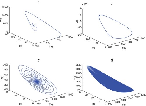
Table 1. List of parameters.

			Value (Unit)
Parameters	Range	Source	Bilinear	Saturation
r	0.03–3 (${\mathrm{d}}^{-1}$)	[1,26]	1	0.5
α	$\ge 1$	[26]	1.2	1.2
$T_{max}$	1000–1500 (${\mathrm{mm}}^{-3}$)	[1,26]	1000	1500
${\beta }_1$	0.000 25–0.5 (${\mathrm{mm}}^3$ ${\mathrm{d}}^{-1}$)	[26]	0.0005	0.02
${\beta }_2$	${10}^{-5}$–10(${\mathrm{mm}}^3$ ${\mathrm{d}}^{-1}$)	[7]	$6.5\times {10}^{-5}$	0.03
c	0.01–10 (${\mathrm{d}}^{-1}$)	[7]	0.05	1
p	0.812 (${\mathrm{d}}^{-1}$)	[26]	0.812	0.812
k	2–1250 (${\mathrm{d}}^{-1}$)	[26]	200	200
$d_1$	0.2–0.5 (${\mathrm{d}}^{-1}$)	[26]	0.4	0.4
$d_2$	2.4–3 (${\mathrm{d}}^{-1}$)	[26]	2.4	2.4
$d_3$	1.618 (${\mathrm{d}}^{-1}$)	[26]	1.618	1.618

5. Control strategy

In this section, we will dedicate to dealing with the optimal control problem by Pontryagin Maximun Principle with delay in state. The interpretation of model (1(1) $\{\begin{array}{l}{\displaystyle \frac{\mathrm{d}T(t)}{\mathrm{d}t}}=rT(t)(1-{\displaystyle \frac{T(t)+\alpha I(t)}{T_{max}}})-f_1(V(t))T(t)-f_2(I(t))T(t),\\ {\displaystyle \frac{\mathrm{d}I(t)}{\mathrm{d}t}}=f_1(V(t))T(t)+f_2(I(t))T(t)-d_{1}I(t)-pI(t)Z(t),\\ {\displaystyle \frac{\mathrm{d}V(t)}{\mathrm{d}t}}=kI(t)-d_{2}V(t),\\ {\displaystyle \frac{\mathrm{d}Z(t)}{\mathrm{d}t}}=cI(t-\tau )-d_{3}Z(t),\end{array}$(1) ) is typical of a disease such as hepatitis B, which is a viral infection that targets the liver. Currently, the therapy for hepatitis B infection focuses on the impairment of viral processes and on the use of immunomodulators, i.e. inhibiting viral production by the antiretroviral nucleside analogues such as tenofovir, entecavir or lamivudine and blocking new infection of the healthy hepatocyte by interferon.

5.1. The optimization problem

To evaluate the efficacy of the two treatments, model (1(1) $\{\begin{array}{l}{\displaystyle \frac{\mathrm{d}T(t)}{\mathrm{d}t}}=rT(t)(1-{\displaystyle \frac{T(t)+\alpha I(t)}{T_{max}}})-f_1(V(t))T(t)-f_2(I(t))T(t),\\ {\displaystyle \frac{\mathrm{d}I(t)}{\mathrm{d}t}}=f_1(V(t))T(t)+f_2(I(t))T(t)-d_{1}I(t)-pI(t)Z(t),\\ {\displaystyle \frac{\mathrm{d}V(t)}{\mathrm{d}t}}=kI(t)-d_{2}V(t),\\ {\displaystyle \frac{\mathrm{d}Z(t)}{\mathrm{d}t}}=cI(t-\tau )-d_{3}Z(t),\end{array}$(1) ) is rewritten as (9) $\{\begin{array}{l}{T}^{\prime }(t)=rT(t)(1-\frac{T(t)+\alpha I(t)}{T_{max}})-(1-u_1(t))f_1(V)T(t)-(1-u_1(t))f_2(I)T(t),\\ I^{\prime }(t)=(1-u_1(t))f_1(V)T(t)+(1-u_1(t))f_2(I)T(t)-d_{1}I(t)-pI(t)Z(t),\\ V^{\prime }(t)=(1-u_2(t))kI(t)-d_{2}V(t),\\ Z^{\prime }(t)=cI(t-\tau )-d_{3}Z(t),\end{array}$(9) with $u_1(t)$ and $u_2(t)$ denoting the functions of time appearing in the time-dependent optimality system, which refer to the therapeutic effects of reducing the risk of transmission and restraining the replication of the virus. Supposing $u_i(t)\in [0,1](i=1,2)$ be Lebesgue integrable on a finite time interval $[t_0,t_f]$, our optimal control problem is to find $u_1(t)$, $u_2(t)$ and the associated state variables such that the following given objective functional can be minimized (10) $J(u_1,u_2)={\int }_{t_0}^{t_f}[I(t)+V(t)+{\displaystyle \frac{B_1}{2}}{u}_1^2(t)+{\displaystyle \frac{B_2}{2}}{u}_2^2(t)]\mathrm{d}t.$(10) The above integrand consists of the number of infected hepatocytes, free virus load and the cost of two treatments, here $B_i(i=1,2)$ denoting the weight constant that reflects the value and the importance of control cost. In addition to be more tractable, the quadratic form of costs is used to model the decreasing efficacy of treatment.

In order to investigate the optimal control of system (9(9) $\{\begin{array}{l}{T}^{\prime }(t)=rT(t)(1-\frac{T(t)+\alpha I(t)}{T_{max}})-(1-u_1(t))f_1(V)T(t)-(1-u_1(t))f_2(I)T(t),\\ I^{\prime }(t)=(1-u_1(t))f_1(V)T(t)+(1-u_1(t))f_2(I)T(t)-d_{1}I(t)-pI(t)Z(t),\\ V^{\prime }(t)=(1-u_2(t))kI(t)-d_{2}V(t),\\ Z^{\prime }(t)=cI(t-\tau )-d_{3}Z(t),\end{array}$(9) ), we first prove that there exists solution of the optimality system such that (11) $J(u_1^{\ast },u_2^{\ast })=\underset{\mathrm{\Omega }}{min}J(u_1(t),u_2(t)),$(11) with $\mathrm{\Omega }=\{(u_1(t),u_2(t))\in L^1(t_0,t_f)|0\le u_1(t),u_2(t)\le 1\}$ being the control set, By the results in [5,15], we have the following theorem.

Theorem 5.1

There exists an optimal solution $u^{\ast }=(u_1^{\ast },u_2^{\ast })$ for the optimal problem (9(9) $\{\begin{array}{l}{T}^{\prime }(t)=rT(t)(1-\frac{T(t)+\alpha I(t)}{T_{max}})-(1-u_1(t))f_1(V)T(t)-(1-u_1(t))f_2(I)T(t),\\ I^{\prime }(t)=(1-u_1(t))f_1(V)T(t)+(1-u_1(t))f_2(I)T(t)-d_{1}I(t)-pI(t)Z(t),\\ V^{\prime }(t)=(1-u_2(t))kI(t)-d_{2}V(t),\\ Z^{\prime }(t)=cI(t-\tau )-d_{3}Z(t),\end{array}$(9) ) such that (11(11) $J(u_1^{\ast },u_2^{\ast })=\underset{\mathrm{\Omega }}{min}J(u_1(t),u_2(t)),$(11) ) is satisfied.

Proof.

It is necessary to verify that the following conditions are satisfied.

1. The control set Ω and the corresponding state variables are nonempty.

2. The control set Ω is convex and closed.

3. The right hand side of the state system is bounded by a linear combination of state and control variables.

4. The integrand $L(I,V,u_1,u_2)=I(t)+V(t)+\frac{B_1}{2}{u}_1^2(t)+\frac{B_2}{2}{u}_2^2(t)$ is concave on Ω.

5. There are positive constants $c_1,c_2>0$ and $\xi >1$ such that $L(I,V,u_1,u_2)\ge c_1+c_2(|u_1{|}^2+|u_2{|}^2{)}^{\frac{\xi }{2}}.$

Based on [15], the boundedness of the state system with strategy of treatment ensures the existence of a solution, which implies that condition (i) is valid. For condition (ii), it is obvious by definition that the control set is bounded and convex. Using the boundedness of the solution and the property of $f_i(i=1,2)$, we know that condition (iii) is satisfied for the form of $u_1$ and $u_2$ in the state system. In order to show the concavity of the integrand L on Ω, its Hessian matrix is given as $H_L=\left(\begin{array}{cc}{B}_1& 0\\ 0& B_2\end{array}\right),$then for any $(u_1,u_2)\in \mathrm{\Omega }$, the determinant of $H_L$ is $det(H_L)=B_1{B}_2\ge 0$ which leads to the condition (iv). Finally, for condition (v), when $c_1$ is taken to be dependent on lower bound of I and V, $c_2=min\{\frac{1}{2}{B}_1,\frac{1}{2}{B}_2\}$, we have $L(I,V,u_1,u_2)\ge c_1+c_2(|u_1{|}^2+|u_2{|}^2).$Accordingly, the existence of optimal control for the minimization problem has been established.

In the following, by optimal control theory and method in [11,20], the therapeutic strategy is analysed to achieve the desired goal of minimizing objective function in (10(10) $J(u_1,u_2)={\int }_{t_0}^{t_f}[I(t)+V(t)+{\displaystyle \frac{B_1}{2}}{u}_1^2(t)+{\displaystyle \frac{B_2}{2}}{u}_2^2(t)]\mathrm{d}t.$(10) ). In fact, the necessary condition of this optimal problem can be generated by dealing with the Hamilton function, which is defined as $H(t)=I(t)+V(t)+{\displaystyle \frac{B_1}{2}}{u}_1^2(t)+{\displaystyle \frac{B_2}{2}}{u}_2^2(t)+\sum _{i=1}^4{\lambda }_i{g}_i,$with $g=(g_1,g_2,g_3,g_4)$ denoting the right-hand side of system (9(9) $\{\begin{array}{l}{T}^{\prime }(t)=rT(t)(1-\frac{T(t)+\alpha I(t)}{T_{max}})-(1-u_1(t))f_1(V)T(t)-(1-u_1(t))f_2(I)T(t),\\ I^{\prime }(t)=(1-u_1(t))f_1(V)T(t)+(1-u_1(t))f_2(I)T(t)-d_{1}I(t)-pI(t)Z(t),\\ V^{\prime }(t)=(1-u_2(t))kI(t)-d_{2}V(t),\\ Z^{\prime }(t)=cI(t-\tau )-d_{3}Z(t),\end{array}$(9) ) and $\lambda =({\lambda }_1,{\lambda }_2,{\lambda }_3,{\lambda }_4)$ being the associated adjoint variable satisfying (12) $\{\begin{array}{l}{\lambda }_1^{\prime }(t)=-{\displaystyle \frac{\mathrm{\partial }H}{\mathrm{\partial }T}},\\ {\lambda }_2^{\prime }(t)=-{\displaystyle \frac{\mathrm{\partial }H}{\mathrm{\partial }I}}-{\chi }_{[t_0,t_f-\tau ]}(t){\displaystyle \frac{\mathrm{\partial }H}{\mathrm{\partial }{I}_{\tau }}}(t+\tau ),\\ {\lambda }_3^{\prime }(t)=-{\displaystyle \frac{\mathrm{\partial }H}{\mathrm{\partial }V}},\\ {\lambda }_4^{\prime }(t)=-{\displaystyle \frac{\mathrm{\partial }H}{\mathrm{\partial }Z}},\end{array}$(12) with the transversality conditions at the final time being ${\lambda }_i(t_f)=0(i=1,2,3,4)$, here $I_{\tau }$ representing delayed state variable of I by $I_{\tau }=I(t-\tau )$, and ${\chi }_{[t_0,t_f-\tau ]}$ being indicator function for the interval $[t_0,t_f-\tau ]$ by ${\chi }_{[t_0,t_f-\tau ]}(t)=\{\begin{array}{ll}1,& \mathrm{if}t\in [t_0,t_f-\tau ],\\ 0,& \mathrm{if}\mathrm{else}.\end{array}$The problem of exploring $u^{\ast }=(u_1^{\ast },u_2^{\ast })$ that minimizes the objective function (10(10) $J(u_1,u_2)={\int }_{t_0}^{t_f}[I(t)+V(t)+{\displaystyle \frac{B_1}{2}}{u}_1^2(t)+{\displaystyle \frac{B_2}{2}}{u}_2^2(t)]\mathrm{d}t.$(10) ) subjected to (9(9) $\{\begin{array}{l}{T}^{\prime }(t)=rT(t)(1-\frac{T(t)+\alpha I(t)}{T_{max}})-(1-u_1(t))f_1(V)T(t)-(1-u_1(t))f_2(I)T(t),\\ I^{\prime }(t)=(1-u_1(t))f_1(V)T(t)+(1-u_1(t))f_2(I)T(t)-d_{1}I(t)-pI(t)Z(t),\\ V^{\prime }(t)=(1-u_2(t))kI(t)-d_{2}V(t),\\ Z^{\prime }(t)=cI(t-\tau )-d_{3}Z(t),\end{array}$(9) ) is converted to minimizing the Hamiltonian with respect to the control, then we have the necessary optimality in the following theorem.

Theorem 5.2

Let $u^{\ast }=(u_1^{\ast },u_2^{\ast })$ be an optimal control and $(\overline{T},\overline{I},\overline{V},\overline{Z})$ be the corresponding solution of (9(9) $\{\begin{array}{l}{T}^{\prime }(t)=rT(t)(1-\frac{T(t)+\alpha I(t)}{T_{max}})-(1-u_1(t))f_1(V)T(t)-(1-u_1(t))f_2(I)T(t),\\ I^{\prime }(t)=(1-u_1(t))f_1(V)T(t)+(1-u_1(t))f_2(I)T(t)-d_{1}I(t)-pI(t)Z(t),\\ V^{\prime }(t)=(1-u_2(t))kI(t)-d_{2}V(t),\\ Z^{\prime }(t)=cI(t-\tau )-d_{3}Z(t),\end{array}$(9) ), then there exists adjoint variable $\overline{\lambda }=({\overline{\lambda }}_1,{\overline{\lambda }}_2,{\overline{\lambda }}_3,{\overline{\lambda }}_4)$ satisfying (12(12) $\{\begin{array}{l}{\lambda }_1^{\prime }(t)=-{\displaystyle \frac{\mathrm{\partial }H}{\mathrm{\partial }T}},\\ {\lambda }_2^{\prime }(t)=-{\displaystyle \frac{\mathrm{\partial }H}{\mathrm{\partial }I}}-{\chi }_{[t_0,t_f-\tau ]}(t){\displaystyle \frac{\mathrm{\partial }H}{\mathrm{\partial }{I}_{\tau }}}(t+\tau ),\\ {\lambda }_3^{\prime }(t)=-{\displaystyle \frac{\mathrm{\partial }H}{\mathrm{\partial }V}},\\ {\lambda }_4^{\prime }(t)=-{\displaystyle \frac{\mathrm{\partial }H}{\mathrm{\partial }Z}},\end{array}$(12) ) such that $H(t,\overline{T},\overline{I},\overline{V},\overline{Z},{\overline{I}}_{\tau },u_1^{\ast },u_2^{\ast },\overline{\lambda })=\underset{\mathrm{\Omega }}{min}H(t,T,I,V,Z,I_{\tau },u_1,u_2,\lambda ).$Moreover, the optimal control is given as (13) $\{\begin{array}{l}{u}_1^{\ast }=max\{min\{{\displaystyle \frac{1}{B_1}}({\overline{\lambda }}_2-{\overline{\lambda }}_1)(f_1(\overline{V})\overline{T}+f_2(\overline{I})\overline{T}),1\},0\},\\ u_2^{\ast }=max\{min\{{\displaystyle \frac{1}{B_2}}k{\overline{\lambda }}_3\overline{I},1\},0\}.\end{array}$(13)

Proof.

Computing for the adjoint system (12(12) $\{\begin{array}{l}{\lambda }_1^{\prime }(t)=-{\displaystyle \frac{\mathrm{\partial }H}{\mathrm{\partial }T}},\\ {\lambda }_2^{\prime }(t)=-{\displaystyle \frac{\mathrm{\partial }H}{\mathrm{\partial }I}}-{\chi }_{[t_0,t_f-\tau ]}(t){\displaystyle \frac{\mathrm{\partial }H}{\mathrm{\partial }{I}_{\tau }}}(t+\tau ),\\ {\lambda }_3^{\prime }(t)=-{\displaystyle \frac{\mathrm{\partial }H}{\mathrm{\partial }V}},\\ {\lambda }_4^{\prime }(t)=-{\displaystyle \frac{\mathrm{\partial }H}{\mathrm{\partial }Z}},\end{array}$(12) ) leads to (14) $\{\begin{array}{ll}{\lambda }_1^{\prime }(t)& =-{\lambda }_{1}r(1-\frac{2T+\alpha I}{T_{max}})+({\lambda }_1-{\lambda }_2)(1-u_1)(f_1(V)+f_2(I)),\\ {\lambda }_2^{\prime }(t)& =-1+{\lambda }_1(\frac{r\alpha T}{T_{max}}+(1-u_1)f_2^{\mathrm{\prime }}(I)T)-{\lambda }_2((1-u_1)f_2^{\prime }(I)T-d_1-pZ)\\ & -{\lambda }_{3}k(1-u_2)-{\chi }_{[t_0,t_f-\tau ]}(t)c{\lambda }_4(t+\tau ),\\ {\lambda }_3^{\prime }(t)& =-1+{\lambda }_1(1-u_1)f_1^{\prime }(V)T-{\lambda }_2(1-u_1)f_1^{\prime }(V)T+{\lambda }_3{d}_2,\\ {\lambda }_4^{\prime }(t)& ={\lambda }_{2}pI+{\lambda }_4{d}_3.\end{array}$(14) By using Pontryagin Maximum Principle, the optimal control $u^{\ast }=(u_1^{\ast },u_2^{\ast })$ can be deduced from the optimality condition ${\displaystyle \frac{\mathrm{\partial }H}{\mathrm{\partial }{u}_1}}=0,{\displaystyle \frac{\mathrm{\partial }H}{\mathrm{\partial }{u}_2}}=0,$that is $\{\begin{array}{l}{B}_1{u}_1+{\lambda }_1{f}_1(V)T+{\lambda }_1{f}_2(I)T-{\lambda }_2{f}_1(V)T-{\lambda }_2{f}_2(I)T=0,\\ B_2{u}_2-{\lambda }_{3}kI=0,\end{array}$from which $u=(u_1,u_2)$ can be solved in terms of state variables and adjoint variables, denoted as $\overline{u}=({\overline{u}}_1,{\overline{u}}_2)$, here $\{\begin{array}{l}{\overline{u}}_1={\displaystyle \frac{1}{B_1}}({\lambda }_2-{\lambda }_1)(f_1(V)T+f_2(I)T),\\ {\overline{u}}_2={\displaystyle \frac{1}{B_2}}k{\lambda }_{3}I.\end{array}$Substituting $\overline{u}=({\overline{u}}_1,{\overline{u}}_2)$ into system (9(9) $\{\begin{array}{l}{T}^{\prime }(t)=rT(t)(1-\frac{T(t)+\alpha I(t)}{T_{max}})-(1-u_1(t))f_1(V)T(t)-(1-u_1(t))f_2(I)T(t),\\ I^{\prime }(t)=(1-u_1(t))f_1(V)T(t)+(1-u_1(t))f_2(I)T(t)-d_{1}I(t)-pI(t)Z(t),\\ V^{\prime }(t)=(1-u_2(t))kI(t)-d_{2}V(t),\\ Z^{\prime }(t)=cI(t-\tau )-d_{3}Z(t),\end{array}$(9) ) and (14(14) $\{\begin{array}{ll}{\lambda }_1^{\prime }(t)& =-{\lambda }_{1}r(1-\frac{2T+\alpha I}{T_{max}})+({\lambda }_1-{\lambda }_2)(1-u_1)(f_1(V)+f_2(I)),\\ {\lambda }_2^{\prime }(t)& =-1+{\lambda }_1(\frac{r\alpha T}{T_{max}}+(1-u_1)f_2^{\mathrm{\prime }}(I)T)-{\lambda }_2((1-u_1)f_2^{\prime }(I)T-d_1-pZ)\\ & -{\lambda }_{3}k(1-u_2)-{\chi }_{[t_0,t_f-\tau ]}(t)c{\lambda }_4(t+\tau ),\\ {\lambda }_3^{\prime }(t)& =-1+{\lambda }_1(1-u_1)f_1^{\prime }(V)T-{\lambda }_2(1-u_1)f_1^{\prime }(V)T+{\lambda }_3{d}_2,\\ {\lambda }_4^{\prime }(t)& ={\lambda }_{2}pI+{\lambda }_4{d}_3.\end{array}$(14) ), we can obtain the corresponding state variables and adjoint variables, denoted as $(\overline{T},\overline{I},\overline{V},\overline{Z})$ and $\overline{\lambda }=({\overline{\lambda }}_1,{\overline{\lambda }}_2,{\overline{\lambda }}_3,{\overline{\lambda }}_4)$ respectively, then we replace them into $\overline{u}$ again, which is still denoted as $\overline{u}$ for convenience. Meanwhile, we need to consider the constrains on the control and the sign of $\mathrm{\partial }H/\mathrm{\partial }u$, i.e. component $u_1^{\ast }$ of the optimal control $u^{\ast }$ can be expressed as follows: $u_1^{\ast }=\{\begin{array}{ll}0,& \mathrm{if}\frac{\mathrm{\partial }H}{\mathrm{\partial }{u}_1}<0,\\ {\overline{u}}_1,& \mathrm{if}\frac{\mathrm{\partial }H}{\mathrm{\partial }{u}_1}=0,\\ 1,& \mathrm{if}\frac{\mathrm{\partial }H}{\mathrm{\partial }{u}_1}>0.\end{array}$For $u_2^{\ast }$, it can be conducted in the similar way, which leads to the expression of the optimal control $u^{\ast }=(u_1^{\ast },u_2^{\ast })$ given in (13(13) $\{\begin{array}{l}{u}_1^{\ast }=max\{min\{{\displaystyle \frac{1}{B_1}}({\overline{\lambda }}_2-{\overline{\lambda }}_1)(f_1(\overline{V})\overline{T}+f_2(\overline{I})\overline{T}),1\},0\},\\ u_2^{\ast }=max\{min\{{\displaystyle \frac{1}{B_2}}k{\overline{\lambda }}_3\overline{I},1\},0\}.\end{array}$(13) ). The proof is completed.

5.2. Simulations of optimality system

In order to perform the numerical simulations, a discretized scheme on the basis of forward and backward finite-difference approximation method is used to solve the optimization system numerically. The bilinear incidence is taken and the parameter values are given the same as in Figure 1(b). We consider the simulation period for 200 days. To compare the numerical results, the simulated procedure is implemented without treatment for the first period of 100 days and with treatment for the second period of 100 days. For the weight coefficients $B_1$ and $B_2$, we take them as $B_1=1000$ and $B_2=1000$, which means that the therapeutic strategy of inhibiting viral production and blocking new infection costs the same. In the following, we mainly consider the implementing of optimal control when there exists periodic solution for model (1(1) $\{\begin{array}{l}{\displaystyle \frac{\mathrm{d}T(t)}{\mathrm{d}t}}=rT(t)(1-{\displaystyle \frac{T(t)+\alpha I(t)}{T_{max}}})-f_1(V(t))T(t)-f_2(I(t))T(t),\\ {\displaystyle \frac{\mathrm{d}I(t)}{\mathrm{d}t}}=f_1(V(t))T(t)+f_2(I(t))T(t)-d_{1}I(t)-pI(t)Z(t),\\ {\displaystyle \frac{\mathrm{d}V(t)}{\mathrm{d}t}}=kI(t)-d_{2}V(t),\\ {\displaystyle \frac{\mathrm{d}Z(t)}{\mathrm{d}t}}=cI(t-\tau )-d_{3}Z(t),\end{array}$(1) ).

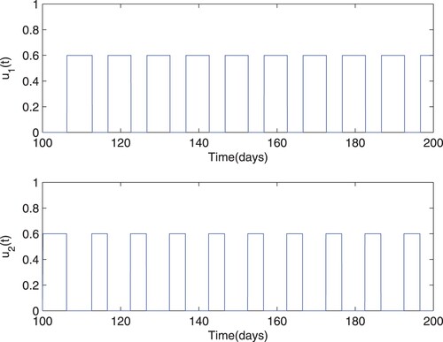
Figure 2 presents the comparison of simulation results in two different cases, i.e. with and without optimal control effect on the bifurcated periodic solution. From the comparison, it can be seen that the application of optimal treatment with $60\mathrm{\%}$ efficacy causes significant quantitative change in the model-simulated consequences of state variables, which specifically results in an increased concentration of target cells and decreased concentrations of infected cells and free virus as well as CTL cells correspondingly. As shown in Figure 2, the solution oscillates in both cases, but the magnitude decreases obviously in the case of implementing control. Meanwhile, with the aim of minimizing the objective functional subject, optimal controls $u_1(t)$ and $u_2(t)$, corresponding to blocking new infections and inhibiting viral production, must be manipulated properly and economically as time evolves, which is plotted in Figure 3. The periodic control curves demonstrate the therapy administration during the given period of 100 days, corresponding to the optimal control in Figure 3 from the start of treatment.

Figure 2. Numerical solution of model (9(9) $\{\begin{array}{l}{T}^{\prime }(t)=rT(t)(1-\frac{T(t)+\alpha I(t)}{T_{max}})-(1-u_1(t))f_1(V)T(t)-(1-u_1(t))f_2(I)T(t),\\ I^{\prime }(t)=(1-u_1(t))f_1(V)T(t)+(1-u_1(t))f_2(I)T(t)-d_{1}I(t)-pI(t)Z(t),\\ V^{\prime }(t)=(1-u_2(t))kI(t)-d_{2}V(t),\\ Z^{\prime }(t)=cI(t-\tau )-d_{3}Z(t),\end{array}$(9) ) with bilinear incidence, the same parameter values as in Figure 1(b) and $0\le u_1(t),u_2(t)\le 0.6$.

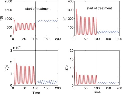
Figure 3. Implementation of the optimal control strategy with time.

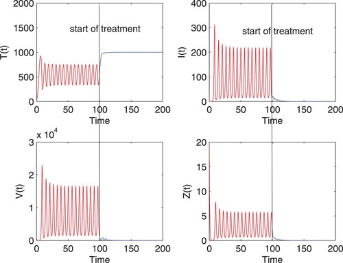
To reveal the effectiveness of optimal control strategy, $90\mathrm{\%}$ efficacy of treatment is also considered, with the same incidence function and parameter values as in Figure 2, which is shown in Figure 4. From the simulation, it can be noted that the application of treatment results in qualitative change in the system dynamics, comparing with that when $60\mathrm{\%}$ efficacy is adopted in Figure 2. As desired, the concentrations of infected cells and free virus are reduced to zero, and the system approaches to a stable disease-free steady state, implying the successful controlling of infection. This figure suggests that the disease clearance can be achieved if the therapeutic efficacy is improved to some high value and $(u_1(t),u_2(t))$ is administrated according to the optimal control solution. However, it is still currently challenging since the available drugs do not directly target cccDNA in chronic hepatitis B and the long-term treatment can lead to the problem of drug resistance.

Figure 4. Numerical solution of model (9(9) $\{\begin{array}{l}{T}^{\prime }(t)=rT(t)(1-\frac{T(t)+\alpha I(t)}{T_{max}})-(1-u_1(t))f_1(V)T(t)-(1-u_1(t))f_2(I)T(t),\\ I^{\prime }(t)=(1-u_1(t))f_1(V)T(t)+(1-u_1(t))f_2(I)T(t)-d_{1}I(t)-pI(t)Z(t),\\ V^{\prime }(t)=(1-u_2(t))kI(t)-d_{2}V(t),\\ Z^{\prime }(t)=cI(t-\tau )-d_{3}Z(t),\end{array}$(9) ) with $0\le u_1(t),u_2(t)\le 0.9$.

6. Conclusion

In this paper, we investigate an in-host DDE model with immune response by incorporating the lag between infection and activation of CTLs. First, dynamical properties of our system are studied analytically. In particular, stability analysis of the steady states has shown that the trivial equilibrium with no biological implication is always unstable, and the endemic equilibrium becomes feasible and probably stable once the infection-free equilibrium loses its stability. When constant time delay is further taken as the bifurcation parameter, the existence of pure imaginary roots of the characteristic equation is verified and the endemic steady state can lose its stability via Hopf bifurcation, resulting in periodic solution, which is presented intuitively in Figure 1.

Furthermore, considering the drug effects in blocking viral production and reducing viral infection for hepatitis B infection, we design an optimal control problem based on the DDE model. Allowing the efficacy of drug combination to vary with time, two control variables needed for optimal therapy are introduced in the system, with one acting as reducing the appearance of new infections in the incidence term, the other one inhibiting viral production in the releasing term for free virus particles. By the optimal control theory and method, we derive the control formulation and use it to search for the best control strategy, i.e. achieving the least amount of liver damage and the lowest cost for the drug combination that lead to hepatitis B virus control. When the bifurcated periodic solution occurs, the comparisons of model-predicted consequences of the state variables are presented numerically with different efficacy ($60\mathrm{\%}$ and $90\mathrm{\%}$), from which the quantitative effects of the control show that the sustained infection can be reduced to a lower level or even to viral clearance, if the control strategy is implemented correspondingly and the rapid progress in the therapy can be achieved.

However, it is known that long-term antiviral therapy results in side effects, compliance and, most importantly, rapid emergence of drug resistance. This has made it difficult to design an optimal control for treatment start, duration, which type of drugs to use and how to assess the effectiveness of treatment measures. Therefore, the limitation in our research can be considered and more accurate models can be developed to characterize the dynamic process and address the optimal control strategy in the presence of these events.

Acknowledgments

This research was supported by National Natural Science Foundation of China under Grant 11801439 and Natural Science Basic Research Plan in Shaanxi Province of China under Grant 2019JM338.

Data availability

The authors confirm that the data supporting the findings of this study are available in our manuscript and within the references.

Disclosure statement

The authors declare that there is no conflict of interest regarding the publication of this paper.

Additional information

Funding

This research was supported by National Natural Science Foundation of China under Grant 11801439 and Natural Science Basic Research Plan in Shaanxi Province of China under Grant 2019JM338.

References

- S. Chen, C. Cheng, and Y. Takeuchi, Stability analysis in delayed within-host viral dynamics with both viral and cellular infections, J. Math. Anal. Appl. 442 (2016), pp. 642–672.
- L. Chen, K. Hattaf, and J. Sun, Optimal control of a delayed SLBS computer virus model, Physica A427 (2015), pp. 244–250.
- J. Danane, A. Meskaf, and K. Allali, Optimal control of a delayed hepaptitis B viral infection model with HBV DNA-containing capsids and CTL immune response, Optim. Control Appl. Methods 39 (2018), pp. 1262–1272.
- P. Das, S. Das, R. Upadhyay, and P. Das, Optimal treatment strategies for delayed cancer-immune system with multiple therapeutic approach, Chaos Solitons Fractals 136 (2020), p. 109806.
- W.H. Fleming and R.W. Rishel, Deterministic and Stochastic Optimal Control, Springer, New York, 1975.
- J. Forde, S. Ciupe, A. Cintron-Arias, and S. Lenhart, Optimal control of drug therapy in a hepatitis B model, Appl. Sci. 6 (2016), pp. 1–18.
- T. Guo, Z. Qiu, and L. Rong, Analysis of an HIV model with immune responses and cell-to-cell transmission, Bull. Malays. Math. Sci. Soc. 43 (2020), pp. 581–607.
- J.K. Hale and S.M. Verduyn Lunel, Introduction to Functional Differential Equations, Springer-Verlag, New York, 1993.
- W.M. Hirsch, H. Hanisch, and J.P. Gabril, Differential equation models of some parasitic infections: Methods for the study of asymptotic behavior, Commun. Pure Appl. Math. 38 (1985), pp. 733–753.
- T. Khan, G. Zaman, and M. Ikhlaq Chohan, The transmission dynamic and optimal control of acute and chronic hepatitis B, J. Biol. Dyn. 11 (2016), pp. 172–189.
- S.M. Lenhart and J.T. Workman, Optimal Control Applied to Biological Models, Taylor & Francis, Boca Raton, 2007.
- M.Y. Li and H. Shu, Multiple stable periodic oscillations in a mathematical model of CTL response to HTLV-I infection, Bull. Math. Biol. 73 (2011), pp. 1774–1793.
- X. Li and J. Wei, On the zeros of a fourth degree exponential polynomial with applications to an eural network model with delays, Chaos Solitons Fractals 26 (2005), pp. 519–526.
- S. Liu, X. Yang, Y. Bi, and Y. Li, Dynamic behavior and optimal scheduling for mixed vaccination strategy with temporary immunity, Discrete Contin. Dyn. Syst. Ser. B 24 (2019), pp. 1469–1483.
- D.L. Lukes, Differential Equations: Classical to Controlled, Academic Press, New York, 1982.
- G. Makay, Uniform boundedness and uniform ultimate boundedness for functional differential equations, Funkc. Ekvacioj 38 (1995), pp. 283–296.
- K. Manna and S.P. Chakrabarty, Global stability of one and two discrete delay models for chronic hepatitis B infection with HBV DNA-containing capsids, Comput. Appl. Math. 36 (2017), pp. 525–536.
- G. Mwanga, H. Haario, and V. Capasso, Optimal control problems of epidemic systems with parameter uncertainties: application to a malaria two-age-class transmission model with asymptomatic carriers, Math. Biosci. 261 (2015), pp. 1–12.
- M.A. Nowak, S. Bonhoeffer, A.M. Hill, R. Boehme, H.C. Thomas, and H. McDade, Viral dynamics in hepatitis B virus infection, Proc. Natl. Acad. Sci. U.S.A. 93 (1996), pp. 4398–4402.
- L. Pontryagin, The Mathematical Theory of Optimal Processed, Taylor & Francis, London, UK, 1987.
- H.L. Smith and X.Q. Zhao, Robust persistence for semidynamical systems, Nonlinear Anal. 47 (2001), pp. 6169–6179.
- H. Song, W. Jiang, and S. Liu, Virus dynamics model with intracellular delays and immune response, Math. Biosci. Eng. 12 (2015), pp. 185–208.
- K. Wang, W. Wang, H. Pang, and X. Liu, Complex dynamic behavior in a viral model with delayed immune response, Physica D 226 (2007), pp. 197–208.
- S. Whang, S. Choi, and E. Jung, A dynamic model for tuberculosis transmission and optimal treatment strategies in South Korea, J. Theor. Biol. 279 (2011), pp. 120–131.
- J. Xu, Y. Geng, and S. Zhang, Global stability and Hopf bifurcation in a delayed viral infection model with cell-to-cell transmission and humoral immune response, Int. J. Bifurcation Chaos 29 (2019), p. 1950161.
- J. Xu and Y. Zhou, Bifurcation analysis of HIV-1 infection model with cell-to-cell transmission and immune response delay, Math. Biosci. Eng. 13 (2016), pp. 343–367.
- Y. Yang, S. Tang, X. Ren, H. Zhao, and C. Guo, Global stability and optimal control for a tuberculosis model with vaccination and treatment, Discrete Contin. Dyn. Syst. Ser. B 21 (2016), pp. 1009–1022.
- Y. Yang, L. Zou, and S. Ruan, Global dynamics of a delayed within-host viral infection model with both virus-to-cell and cell-to-cell transmissions, Math. Biosci. 270 (2015), pp. 183–191.
- S. Zhang and X. Xu, Dynamic analysis and optimal control for a model of hepatitis C with treatment, Commun. Nonlinear Sci. Numer. Simul. 46 (2017), pp. 14–25.
- H. Zhang, Z. Yang, K. Pawelek, and S. Liu, Optimal control strategies for a two-group epdiemic model with vaccination-resource constrains, Appl. Math. Comput. 371 (2019), p. 124956.
- H. Zhu, Y. Luo, and M. Chen, Stability and Hopf bifurcation of a HIV infection model with CTL-response delay, Comput. Math. Appl. 62 (2011), pp. 3091–3102.