A mathematical model for tilapia lake virus transmission with waning immunity

Abstract

The goal of this paper is to investigate the influence of the waning immunity on the dynamics of Tilapia Lake Virus (TiLV) transmission in wild and farmed tilapia within freshwater. We formulate a model for which susceptible individuals can contract the disease in two ways: (i) direct mode caused by contact with infected individuals; (ii) indirect mode due to the presence of pathogenic agents in the water. We obtain an age-structured model which combines both age since infection and age since recovery. We derive an explicit formula for the reproductive number ${\mathcal{R}}_0$ and show that the disease-free equilibrium is locally asymptotically stable when, ${\mathcal{R}}_0<1$. We discuss on the form of the waning immunity parameter and show numerically that a Hopf bifurcation may occur for suitable immunity parameter values, which means that there is a periodic solution around the endemic equilibrium when, ${\mathcal{R}}_0>1$.

Keywords:

• Age-structured model
• tilapia lake virus (TiLV)
• basic reproduction number
• stability
• waning immunity

Mathematics Subject Classifications:

• 45K05
• 45M10
• 92D25
• 92D30

1. Introduction

The immune system can be categorized into specific (adaptive) immunity with immunological memory and non-specific innate immunity [14,23,34]. The specific immune system involves the recognition of specific antigens on a pathogen, thereby providing protection against that pathogen primarily in the form of specific antibodies. In contrast, the non-specific immune system provides an array of protective mechanisms that are inherently available and provide immediate and permanent protection against a wide variety of pathogen. Therefore, the adaptive immune response is activated by the innate immune system in order to allow a specific response [31].

Further, the innate parameters are at the forefront of host immune defense and are a crucial factor in disease resistance. The adaptive response is commonly delayed but is essential for long-lasting immunity and a key factor in successful vaccination. Both innate and adaptive immunities complement each other in the host's attempt to prevent infection [14]. A key feature of the adaptive immune system is immunological memory. Repeat infections by the same virus or bacteria induce a strong and specific response that usually stops the infection and has less reliance on the innate system. Vaccination against infection is possible due to this immune memory. The first adaptive response against an infection, called the primary response, often takes days to mature. In contrast, a memory response develops within hours of infection. Memory is maintained by a subset of B and T lymphocytes called memory cells, which can potentially survive for years in the body. Memory cells remain ready to respond rapidly and efficiently to a subsequent encounter with a pathogen, giving rise to stronger and faster so-called secondary responses [20]. Most animals are susceptible to the initial infection, but they differ in their ability to limit the infection or destroy the pathogen [29].

Tilapia is considered as the second largest farmed fish species after carp globally. With such expansion, there is the risk of emergence of infectious diseases and tilapia lake virus infection has been shown to cause high mortalities ( 20–90%) over the last 4–5 years [4,12,25]. The identified routes of transmission are: horizontally through cohabitation [13], and vertically, that is from infected fish to their offspring [11,35]. Recently Tattiyapong et al. in [33], showed that the tilapia can develop protective immunity including a humoral response following exposure to TiLV. In this paper, we devote our attention to the modelling of an age-structured model for TiLV transmission that incorporates both horizontal direct (contact), indirect (through water) transmission routes, and waning immunity. To the best of our knowledge, only two mathematical papers have been devoted to understand the dynamics of the TiLV transmission. Their authors use various mathematical approaches: ordinary differential equation [36] and partial differential equation [19]. The model developed here can be viewed as an extension of the one in [19] in the following sense:

• According to [9,18], the death rate in tilapia fisheries was reported to be density-dependent. So, to be more realistic, we consider two types of mortality rates: the density non-dependent and the density-dependent mortality.

• Though the dynamics of immune status among host individuals plays a crucial role in the spread of infectious disease, Tattiyapong et al. [33] showed that TiLV infection provides recovered individuals with a short or relatively long immunity against re-infection and they lose their immunity through time, allowing them to become susceptible again. This means that it is natural for us to include the effects of immunity into our model in order to better represent the actual dynamics of TiLV epidemic spread and predict future outbreaks.

Furthermore, several papers have investigated diseases transmission with age of infection [3,7,8,19,21,24,37]. But, only few have addressed models with both time since infection and waning immunity. S. Bhattacharya and F.R. Adler [5] considered a SIRS model with temporary immunity when the rate of loss of immunity can depend on the time since recovery from disease. They determined the conditions under which the endemic steady state becomes unstable and found that rapid immunity loss is necessary to produce oscillations. In [17], H. Gulbudak et al. developed an immuno-epidemiological model that links the within-host dynamics to between-host circulation of a vector-borne disease. They derived evolutionary optimization principles for both pathogen and host and obtained by the invasion analysis that the ${\mathcal{R}}_0$ maximization principle holds for the vector-borne pathogen. For the host, they find that increasing the vector inoculum size increases the pathogen ${\mathcal{R}}_0$, but can either increase or decrease the pathogen virulence, suggesting that vector inoculum size can contribute to the virulence of vector-borne diseases in distinct ways.

More recently, R. Djidjou-Demasse et al. [30] considered a human-vector malaria transmission model structured by age, time since infection and waning immunity. They proved the existence of equilibria and obtained a necessary and sufficient condition that implies the bifurcation of the endemic equilibria. They also proved that by neglecting the age dependence of the human population, and under some certain conditions, they may be a backward or a forward bifurcation.

The present article considers an age-structured model with loss of immunity, which is considered to be one of the sources causing recurrence of infectious disease dynamics observed in many epidemics. Every recovered individual losses progressively its immunity, implying its direct reversion from the recovered class to the susceptible class at a rate that depends upon time since recovery. The obtained system is a SIVRS model, including two hyperbolic first-order partial differential equations coupled with two ordinary differential equations. Using the integrated semi-group theory [22,24], we prove some well-posedness results. We obtain an explicit formula for the basic reproduction number ${\mathcal{R}}_0$, we show the existence of a unique disease-free equilibrium and obtain its local stability. Finally, we explore the role of waning immunity on the epidemic evolution.

The organization of this paper is as follows. In Section 2, we formulate the model and prove its mathematical well-posedness. Section 3 is devoted to the computation of the basic reproduction number, the disease-free equilibrium and its stability. In Section 4, we perform some numerical simulations. In Section 5, a brief discussion is given to end this work.

2. Model and its mathematical well-posedness

2.1. Model formulation

Let $S(t)$ be the density of susceptible fish at time t, $i(a,t)$ the density of fish infected at time t with respect to age of infection a and $r(\tau ,t)$ be the density of recovered fish at time t with respect to the time since recovery τ. We denote by $V(t)$, the pathogen concentration in a water source at time t. The birth rate in the population is denoted by b. The constant ${\sigma }^{ind}$ denotes the transmission rate parameter for water-to-fish contact (horizontal indirect transmission). The density non-dependent and dependent mortality rates are denoted by ${\mu }_0$ and ${\mu }_1$ respectively. During an infection, fish can either die from infection at a rate ${\mu }_i(a)$, or recover at a time since infection a with a rate $\delta (a)$. A recovered fish loses its immunity at a rate $\gamma (\tau )$. The proportion of offspring born in the infected class is denoted by $\pi (a)\in [0,1]$, and we assume that offspring from the recovered class are born susceptible. Then the terms ${\displaystyle b{\int }_0^{\mathrm{\infty }}\pi (a)i(a,t)\mathrm{d}a}$ denotes the flux of infected offspring born into the infected class at time t. The term $\beta (a)i(a,t)$ represents the flux of pathogen shed by infected fish with respect to the age of their infection at time t. The flux of shed pathogen a time t is modelled by the term ${\displaystyle {\int }_0^{\mathrm{\infty }}\beta (a)i(a,t)\mathrm{d}a}$, we assume that a fraction $p\in [0,1]$ of this flux, is directly ingested by fish at time t by direct contact (from fish to fish) with a rate ${\sigma }^{dir}$ and the remaining 1−p is shed in water. The flux of newly infected fish corresponds to the boundary condition for i at age a = 0, while the flux of newly recovered fish corresponds to the boundary condition for r at $\tau =0$. The mortality rate of the virus is denoted by ${\mu }_V$. The total number of infected individuals is $I(t)={\int }_0^{\mathrm{\infty }}i(a,t)\mathrm{d}a$, while the total number of recovered individual is $R(t)={\int }_0^{\mathrm{\infty }}r(\tau ,t)\mathrm{d}\tau$. Then the total size of population at time t is given by $N(t)=S(t)+I(t)+R(t)$. With all the above notations, the model reads as follows (1) $\begin{array}{r}\{\begin{array}{l}{\displaystyle \frac{\mathrm{d}S(t)}{\mathrm{d}t}=(b-J(t)-({\mu }_0+{\mu }_{1}N(t)))S(t)+bR(t)}\\ +b{\int }_0^{\mathrm{\infty }}(1-\pi (a))i(a,t)\mathrm{d}a+{\int }_0^{\mathrm{\infty }}\gamma (\tau )r(\tau ,t)\mathrm{d}\tau ,\\ {\displaystyle \frac{\mathrm{\partial }i(a,t)}{\mathrm{\partial }t}+\frac{\mathrm{\partial }i(a,t)}{\mathrm{\partial }a}=-(\delta (a)+{\mu }_i(a)+{\mu }_0+{\mu }_{1}N(t))i(a,t),}\\ {\displaystyle \frac{\mathrm{\partial }r(\tau ,t)}{\mathrm{\partial }t}+\frac{\mathrm{\partial }r(\tau ,t)}{\mathrm{\partial }\tau }=-(\gamma (\tau )+{\mu }_0+{\mu }_{1}N(t))r(\tau ,t),}\\ {\displaystyle \frac{\mathrm{d}V(t)}{\mathrm{d}t}=(1-p){\int }_0^{\mathrm{\infty }}\beta (a)i(a,t)\mathrm{d}a-{\mu }_{V}V(t),}\end{array}\end{array}$(1) where (2) $\begin{array}{r}J(t)={\sigma }^{ind}V(t)+p{\sigma }^{dir}{\int }_0^{\mathrm{\infty }}\beta (a)i(a,t)\mathrm{d}a,\end{array}$(2) with boundary conditions (3) $\begin{array}{r}\begin{array}{l}{\displaystyle i(0,t)=J(t)S(t)+b{\int }_0^{\mathrm{\infty }}\pi (a)i(a,t)\mathrm{d}a,}\\ r(0,t)={\displaystyle {\int }_0^{\mathrm{\infty }}\delta (a)i(a,t)\mathrm{d}a,}\end{array}\end{array}$(3) and the following initial conditions (4) $\begin{array}{r}\begin{array}{l}S(0)=S_0,i(a,0)=i_0(a),r(\tau ,0)=r_0(\tau )\mathrm{and}V(0)=V_0.\end{array}\end{array}$(4)

Assumption 2.1

We make the following assumptions

1. $b,{\mu }_0,{\mu }_1,{\mu }_V,{\sigma }^{dir},{\sigma }^{ind}>0$ with $b>{\mu }_0$;

2. The functions $\delta (\cdot ),{\mu }_i(\cdot ),\gamma (\cdot )\in L_{+}^{\mathrm{\infty }}(0,\mathrm{\infty })$ and $\gamma (\tau )>{\gamma }_0$, for a.e $\tau \in (0,\mathrm{\infty })$ and for some ${\gamma }_0>0$;

3. The functions $\beta (.),{\pi }_i(.)$ are positive, bounded and uniformly continuous on $(0,\mathrm{\infty })$. And there exists a positive constant ${\pi }_0$ such that $\pi (a)\ge {\pi }_0$ for a.e $a\in (0,\mathrm{\infty })$;

4. The initial conditions are such that $S_0,V_0>0$, $i_0(\cdot ),r_0(\cdot )\in L_{+}^1(0,\mathrm{\infty })$.

2.2. Mathematical well-posedness

In this section, we prove that the system (1(1) $\begin{array}{r}\{\begin{array}{l}{\displaystyle \frac{\mathrm{d}S(t)}{\mathrm{d}t}=(b-J(t)-({\mu }_0+{\mu }_{1}N(t)))S(t)+bR(t)}\\ +b{\int }_0^{\mathrm{\infty }}(1-\pi (a))i(a,t)\mathrm{d}a+{\int }_0^{\mathrm{\infty }}\gamma (\tau )r(\tau ,t)\mathrm{d}\tau ,\\ {\displaystyle \frac{\mathrm{\partial }i(a,t)}{\mathrm{\partial }t}+\frac{\mathrm{\partial }i(a,t)}{\mathrm{\partial }a}=-(\delta (a)+{\mu }_i(a)+{\mu }_0+{\mu }_{1}N(t))i(a,t),}\\ {\displaystyle \frac{\mathrm{\partial }r(\tau ,t)}{\mathrm{\partial }t}+\frac{\mathrm{\partial }r(\tau ,t)}{\mathrm{\partial }\tau }=-(\gamma (\tau )+{\mu }_0+{\mu }_{1}N(t))r(\tau ,t),}\\ {\displaystyle \frac{\mathrm{d}V(t)}{\mathrm{d}t}=(1-p){\int }_0^{\mathrm{\infty }}\beta (a)i(a,t)\mathrm{d}a-{\mu }_{V}V(t),}\end{array}\end{array}$(1) )–(4(4) $\begin{array}{r}\begin{array}{l}S(0)=S_0,i(a,0)=i_0(a),r(\tau ,0)=r_0(\tau )\mathrm{and}V(0)=V_0.\end{array}\end{array}$(4) ) is well posed by using an integrated semi-group approach [21,24]. Before going further, we introduce the space $X_1$ defined by $X_1=\mathbb{R}\times L^1(0,\mathrm{\infty }).$

Let $A_i:D(A_i)\subset X_1\to X_1$ and $A_r:D(A_r)\subset X_1\to X_1$ be two linear operators on $X_1$ defined by $\begin{array}{rl}{A}_i\left(\begin{array}{c}0\\ \phi \end{array}\right)& =\left(\begin{array}{c}-\phi (0)\\ -({\displaystyle \frac{\mathrm{\partial }}{\mathrm{\partial }a}}+\delta (a)+{\mu }_i(a)+{\mu }_0)\phi \end{array}\right),\\ A_r\left(\begin{array}{c}0\\ \varphi \end{array}\right)& =\left(\begin{array}{c}-\varphi (0)\\ -(\frac{\mathrm{\partial }}{\mathrm{\partial }\tau }+\gamma (\tau )+{\mu }_0)\varphi \end{array}\right),\end{array}$with $D(A_i)=D(A_r)=\{0\}\times W^{1,1}(0,\mathrm{\infty }).$

Next, let $\mathbb{X}$ be the space defined by $\mathbb{X}=\mathbb{R}\times X_1\times X_1\times \mathbb{R}$

We define on $\mathbb{X}$ the norm, for $\phi =({\phi }_1,{\phi }_2,{\phi }_3,{\phi }_4,{\phi }_5,{\phi }_6{)}^T\in \mathbb{X}$, $\Vert \phi {\Vert }_{\mathbb{X}}=|{\phi }_1|+|{\phi }_2|+{\int }_0^{\mathrm{\infty }}|{\phi }_3(a)|\mathrm{d}a+|{\phi }_4|+{\int }_0^{\mathrm{\infty }}|{\phi }_5(\tau )|\mathrm{d}\tau +|{\phi }_6|.$

It is clear that $\mathbb{X}$ endowed with the norm $\Vert \cdot {\Vert }_{\mathbb{X}}$ is a Banach space. We denote by ${\mathbb{X}}_{+}$ the positive cone of $\mathbb{X}$, that is ${\mathbb{X}}_{+}={\mathbb{R}}_{+}\times X_{1,+}\times X_{1,+}\times {\mathbb{R}}_{+}.$

Let also ${\mathbb{X}}_0=\mathbb{R}\times \{0\}\times L^1(0,\mathrm{\infty })\times \{0\}\times L^1(0,\mathrm{\infty })\times \mathbb{R}$ and define the linear operator $A:D(A)\subset \mathbb{X}\to \mathbb{X}$ by $A=\left[\begin{array}{cccc}b-{\mu }_0& 0& 0& 0\\ 0& A_i& 0& 0\\ 0& 0& A_r& 0\\ 0& 0& 0& -{\mu }_V\end{array}\right]$with $D(A)=\mathbb{R}\times D(A_i)\times D(A_r)\times \mathbb{R}.$

Then $\overline{D(A)}={\mathbb{X}}_0$ is not dense in $\mathbb{X}$. For $v(t)=(S(t),0,i(\cdot ,t),0,r(\cdot ,t),V(t){)}^T$, let $\begin{array}{rl}{\displaystyle F_1(v(t))}& =-(J(t)+{\mu }_{1}N(t))S(t)+bR(t)\\ & +b{\int }_0^{\mathrm{\infty }}(1-\pi (a))i(a,t)\mathrm{d}a+{\int }_0^{\mathrm{\infty }}\gamma (\tau )r(\tau ,t)\mathrm{d}\tau ,\\ {\displaystyle F_2(v(t))}& =J(t)S(t)+b{\int }_0^{\mathrm{\infty }}\pi (a)i(a,t)\mathrm{d}a,\\ {\displaystyle F_3(v(t))}& ={\mu }_{1}N(t)i(.,t),\\ {\displaystyle F_4(v(t))}& ={\int }_0^{\mathrm{\infty }}\delta (a)i(a,t)\mathrm{d}a,\\ {\displaystyle F_5(v(t))}& ={\mu }_{1}N(t)r(.,t),\end{array}$and ${\displaystyle F_6(v(t))=(1-p){\int }_0^{\mathrm{\infty }}\beta (a)i(a,t)\mathrm{d}a.}$

We consider $F:\overline{D(A)}\to \mathbb{X}$ the nonlinear map defined by $F(v(t))=\left(\begin{array}{c}{F}_1(v(t))\\ F_2(v(t))\\ F_3(v(t))\\ F_4(v(t))\\ F_5(v(t))\\ F_6(v(t))\end{array}\right).$

Set ${\mathbb{X}}_0^{+}={\mathbb{X}}_0\cap {\mathbb{X}}_{+}$. Then, the system (1(1) $\begin{array}{r}\{\begin{array}{l}{\displaystyle \frac{\mathrm{d}S(t)}{\mathrm{d}t}=(b-J(t)-({\mu }_0+{\mu }_{1}N(t)))S(t)+bR(t)}\\ +b{\int }_0^{\mathrm{\infty }}(1-\pi (a))i(a,t)\mathrm{d}a+{\int }_0^{\mathrm{\infty }}\gamma (\tau )r(\tau ,t)\mathrm{d}\tau ,\\ {\displaystyle \frac{\mathrm{\partial }i(a,t)}{\mathrm{\partial }t}+\frac{\mathrm{\partial }i(a,t)}{\mathrm{\partial }a}=-(\delta (a)+{\mu }_i(a)+{\mu }_0+{\mu }_{1}N(t))i(a,t),}\\ {\displaystyle \frac{\mathrm{\partial }r(\tau ,t)}{\mathrm{\partial }t}+\frac{\mathrm{\partial }r(\tau ,t)}{\mathrm{\partial }\tau }=-(\gamma (\tau )+{\mu }_0+{\mu }_{1}N(t))r(\tau ,t),}\\ {\displaystyle \frac{\mathrm{d}V(t)}{\mathrm{d}t}=(1-p){\int }_0^{\mathrm{\infty }}\beta (a)i(a,t)\mathrm{d}a-{\mu }_{V}V(t),}\end{array}\end{array}$(1) )–(4(4) $\begin{array}{r}\begin{array}{l}S(0)=S_0,i(a,0)=i_0(a),r(\tau ,0)=r_0(\tau )\mathrm{and}V(0)=V_0.\end{array}\end{array}$(4) ) rewrites as the following abstract Cauchy problem (5) $\begin{array}{r}\frac{\mathrm{d}v(t)}{\mathrm{d}t}=Av(t)+F(v(t)),\mathrm{for}t\ge 0,\mathrm{with}v(0)=v_0\in {\mathbb{X}}_0^{+},\end{array}$(5) where $v_0=(S_0,0,i_0,0,r_0,V_0{)}^T.$ In general, the differential Equation (5(5) $\begin{array}{r}\frac{\mathrm{d}v(t)}{\mathrm{d}t}=Av(t)+F(v(t)),\mathrm{for}t\ge 0,\mathrm{with}v(0)=v_0\in {\mathbb{X}}_0^{+},\end{array}$(5) ) may not have a strong solution. Thus, we solve it in integrated form: (6) $\begin{array}{r}v(t)=v_0+A{\int }_0^{t}v(s)\mathrm{d}s+{\int }_0^{t}F(v(s))\mathrm{d}s.\end{array}$(6)

A continuous solution to (5(5) $\begin{array}{r}\frac{\mathrm{d}v(t)}{\mathrm{d}t}=Av(t)+F(v(t)),\mathrm{for}t\ge 0,\mathrm{with}v(0)=v_0\in {\mathbb{X}}_0^{+},\end{array}$(5) ) is called an integral solution to (6(6) $\begin{array}{r}v(t)=v_0+A{\int }_0^{t}v(s)\mathrm{d}s+{\int }_0^{t}F(v(s))\mathrm{d}s.\end{array}$(6) ). The next result states the well posedness of (1(1) $\begin{array}{r}\{\begin{array}{l}{\displaystyle \frac{\mathrm{d}S(t)}{\mathrm{d}t}=(b-J(t)-({\mu }_0+{\mu }_{1}N(t)))S(t)+bR(t)}\\ +b{\int }_0^{\mathrm{\infty }}(1-\pi (a))i(a,t)\mathrm{d}a+{\int }_0^{\mathrm{\infty }}\gamma (\tau )r(\tau ,t)\mathrm{d}\tau ,\\ {\displaystyle \frac{\mathrm{\partial }i(a,t)}{\mathrm{\partial }t}+\frac{\mathrm{\partial }i(a,t)}{\mathrm{\partial }a}=-(\delta (a)+{\mu }_i(a)+{\mu }_0+{\mu }_{1}N(t))i(a,t),}\\ {\displaystyle \frac{\mathrm{\partial }r(\tau ,t)}{\mathrm{\partial }t}+\frac{\mathrm{\partial }r(\tau ,t)}{\mathrm{\partial }\tau }=-(\gamma (\tau )+{\mu }_0+{\mu }_{1}N(t))r(\tau ,t),}\\ {\displaystyle \frac{\mathrm{d}V(t)}{\mathrm{d}t}=(1-p){\int }_0^{\mathrm{\infty }}\beta (a)i(a,t)\mathrm{d}a-{\mu }_{V}V(t),}\end{array}\end{array}$(1) )–(4(4) $\begin{array}{r}\begin{array}{l}S(0)=S_0,i(a,0)=i_0(a),r(\tau ,0)=r_0(\tau )\mathrm{and}V(0)=V_0.\end{array}\end{array}$(4) ).

Theorem 2.1

The system of Equations (1(1) $\begin{array}{r}\{\begin{array}{l}{\displaystyle \frac{\mathrm{d}S(t)}{\mathrm{d}t}=(b-J(t)-({\mu }_0+{\mu }_{1}N(t)))S(t)+bR(t)}\\ +b{\int }_0^{\mathrm{\infty }}(1-\pi (a))i(a,t)\mathrm{d}a+{\int }_0^{\mathrm{\infty }}\gamma (\tau )r(\tau ,t)\mathrm{d}\tau ,\\ {\displaystyle \frac{\mathrm{\partial }i(a,t)}{\mathrm{\partial }t}+\frac{\mathrm{\partial }i(a,t)}{\mathrm{\partial }a}=-(\delta (a)+{\mu }_i(a)+{\mu }_0+{\mu }_{1}N(t))i(a,t),}\\ {\displaystyle \frac{\mathrm{\partial }r(\tau ,t)}{\mathrm{\partial }t}+\frac{\mathrm{\partial }r(\tau ,t)}{\mathrm{\partial }\tau }=-(\gamma (\tau )+{\mu }_0+{\mu }_{1}N(t))r(\tau ,t),}\\ {\displaystyle \frac{\mathrm{d}V(t)}{\mathrm{d}t}=(1-p){\int }_0^{\mathrm{\infty }}\beta (a)i(a,t)\mathrm{d}a-{\mu }_{V}V(t),}\end{array}\end{array}$(1) )–(4(4) $\begin{array}{r}\begin{array}{l}S(0)=S_0,i(a,0)=i_0(a),r(\tau ,0)=r_0(\tau )\mathrm{and}V(0)=V_0.\end{array}\end{array}$(4) ) represented by the integral Equation (6(6) $\begin{array}{r}v(t)=v_0+A{\int }_0^{t}v(s)\mathrm{d}s+{\int }_0^{t}F(v(s))\mathrm{d}s.\end{array}$(6) ) has a unique continuous solution with values in ${\mathbb{X}}_0^{+}$ and the map $\mathrm{\Psi }:[0,\mathrm{\infty })\times {\mathbb{X}}_0^{+}\to {\mathbb{X}}_0^{+}$ defined by ${\displaystyle \mathrm{\Psi }(t,x):=(S(t),0,i(\cdot ,t),0,r(\cdot ,t),V(t){)}^T}$ is a continuous semiflow. That is the map Ψ is continuous and $\mathrm{\Psi }(t,\mathrm{\Psi }(s,.))=\mathrm{\Psi }(t+s,.)$ and $\mathrm{\Psi }(0,.)$ is the identity map.

Proof.

We proceed as in [24]. First, it is easy to see that the function F is Lipschitz continuous on bounded sets. Next, we prove that the operator $(A,D(A))$ is a Hille–Yosida operator and $(\lambda -A{)}^{-1}$ maps ${\mathbb{X}}_{+}$ into itself (A is resolvent positive). Indeed let $\lambda >-\tilde{\mu }:=-min\{b-{\mu }_0,{\gamma }_0,{\mu }_V\}$, $f=(\phi ,\mathrm{\Phi },\varphi ,\mathrm{\Psi },\psi ,\omega )\in \mathbb{X}$ and $g=(\tilde{\phi },(0,\tilde{\varphi }),(0,\tilde{\psi }),\tilde{\omega })\in D(A)$. Then $(\lambda -A{)}^{-1}\left(\begin{array}{c}\phi \\ \mathrm{\Phi }\\ \varphi \\ \mathrm{\Psi }\\ \psi \\ \omega \end{array}\right)=\left(\begin{array}{c}\tilde{\phi }\\ \left(\begin{array}{c}0\\ \tilde{\varphi }\end{array}\right)\\ \left(\begin{array}{c}0\\ \tilde{\psi }\end{array}\right)\\ \tilde{\omega }\end{array}\right)⟺\{\begin{array}{l}{\displaystyle (\lambda -b+{\mu }_0)\tilde{\phi }=\phi ,}\\ \tilde{\varphi }(0)=\mathrm{\Phi },\\ {\displaystyle \frac{\mathrm{d}}{\mathrm{d}a}\tilde{\varphi }+(\lambda +\delta (a)+{\mu }_i(a)+{\mu }_0)\tilde{\varphi }=\varphi ,}\\ \tilde{\psi }(0)=\mathrm{\Psi },\\ {\displaystyle \frac{\mathrm{d}}{\mathrm{d}\tau }\tilde{\psi }+(\lambda +\gamma (\tau ))\tilde{\psi }=\psi ,}\\ (\lambda +{\mu }_V)\tilde{\omega }=\omega .\end{array}$

Solving this latter system of equation lead us to (7) $\begin{array}{r}\{\begin{array}{l}{\displaystyle \tilde{\phi }=\frac{\phi }{\lambda -b+{\mu }_0},}\\ {\displaystyle \tilde{\varphi }=\mathrm{\Phi }{e}^{-(\lambda +{\mu }_0)a}{e}^{-{\int }_0^a(\delta (s)+{\mu }_i(s))\mathrm{d}s}+{\int }_0^a\varphi (s)e^{-(\lambda +{\mu }_0)(a-s)}{e}^{-{\int }_s^a(\delta (\sigma )+{\mu }_i(\sigma ))\mathrm{d}\sigma }\mathrm{d}a,}\\ {\displaystyle \tilde{\psi }=\mathrm{\Psi }{e}^{-\lambda \tau }{e}^{-{\int }_0^{\tau }\gamma (s)\mathrm{d}s}+{\int }_0^{\tau }\psi (s)e^{-\lambda (\tau -s)}{e}^{-{\int }_s^{\tau }\gamma (\sigma )\mathrm{d}\sigma }\mathrm{d}\tau ,}\\ {\displaystyle \tilde{\omega }=\frac{\omega }{\lambda +{\mu }_V}.}\end{array}\end{array}$(7)

Integrating the equations for $\tilde{\varphi }$ and for $\tilde{\psi }$ with respect to a and τ, respectively, and adding all obtained equations yields $\begin{array}{rl}& |\tilde{\phi }|+\Vert \tilde{\varphi }{\Vert }_{L^1(0,\mathrm{\infty })}+\Vert \tilde{\psi }{\Vert }_{L^1(0,\mathrm{\infty })}+|\tilde{\omega }|\\ & \le \frac{1}{\lambda +\tilde{\mu }}(|\phi |+|\mathrm{\Phi }|+\Vert \varphi {\Vert }_{L^1(0,\mathrm{\infty })}+|\mathrm{\Psi }|+\Vert \psi {\Vert }_{L^1(0,\mathrm{\infty })}+|\omega |).\end{array}$So $\Vert (\lambda -A{)}^{-1}\Vert \le \frac{1}{\lambda +\tilde{\mu }}.$

Hence A is Hille–Yosida. Moreover, if we assume that $f\in {\mathcal{X}}_{+}$, then by (7(7) $\begin{array}{r}\{\begin{array}{l}{\displaystyle \tilde{\phi }=\frac{\phi }{\lambda -b+{\mu }_0},}\\ {\displaystyle \tilde{\varphi }=\mathrm{\Phi }{e}^{-(\lambda +{\mu }_0)a}{e}^{-{\int }_0^a(\delta (s)+{\mu }_i(s))\mathrm{d}s}+{\int }_0^a\varphi (s)e^{-(\lambda +{\mu }_0)(a-s)}{e}^{-{\int }_s^a(\delta (\sigma )+{\mu }_i(\sigma ))\mathrm{d}\sigma }\mathrm{d}a,}\\ {\displaystyle \tilde{\psi }=\mathrm{\Psi }{e}^{-\lambda \tau }{e}^{-{\int }_0^{\tau }\gamma (s)\mathrm{d}s}+{\int }_0^{\tau }\psi (s)e^{-\lambda (\tau -s)}{e}^{-{\int }_s^{\tau }\gamma (\sigma )\mathrm{d}\sigma }\mathrm{d}\tau ,}\\ {\displaystyle \tilde{\omega }=\frac{\omega }{\lambda +{\mu }_V}.}\end{array}\end{array}$(7) ), we obtain $\tilde{\phi }\ge 0,\tilde{\varphi }\ge 0,\tilde{\omega }\ge 0$ and $\tilde{\omega }\ge 0$. That is $g=(\tilde{\phi },(0,\tilde{\varphi }),(0,\tilde{\psi }),\tilde{\omega })\in {\mathbb{X}}_{+}$. Thus $(\lambda -A{)}^{-1}$ maps ${\mathbb{X}}_{+}$ into ${\mathbb{X}}_{+}$. Next we show that for all $t\ge 0$ and $v\in {\mathbb{X}}_0^{+}$, (8) $\begin{array}{r}\underset{h\to 0^{+}}{lim}\frac{1}{h}dist(v+hF(v),{\mathbb{X}}_{+})=0,\end{array}$(8) where ${\displaystyle dist(v,{\mathbb{X}}_{+})=\underset{u\in {\mathbb{X}}_{+}}{inf}\Vert v-u{\Vert }_{\mathbb{X}}}$. Let m>0 and $B(0,m)$ be the ball of $\mathbb{X}$ centered at 0 and with radius m. By the expression of F, there exists a positive constant $C=C(m,\Vert \beta {\Vert }_{L^{\mathrm{\infty }}(0,\mathrm{\infty })})$ such for any $v\in {\mathbb{X}}_0^{+}\cap B(0,m)$, $F(v)+\alpha v\in {\mathbb{X}}_{+}.$

Now, if we let $\tilde{F}(v)=F(v)+\alpha v,$with α being chosen such that $\alpha >C$. Then $\tilde{F}(v)\in {\mathbb{X}}_{+}$ and for any positive and sufficiently small h, we have $\alpha -\alpha hv\in {\mathbb{X}}_{+}$ and $h\tilde{F}(v)\in {\mathbb{X}}_{+}$. So ${\displaystyle \underset{h\to 0^{+}}{lim}\frac{1}{h}dist(v+hF(v),{\mathbb{X}}_{+})=\underset{h\to 0^{+}}{lim}\frac{1}{h}dist(\alpha -\alpha hv+h\tilde{F}(v),{\mathbb{X}}_{+})=0.}$

In what follows, we prove that the solution of (1(1) $\begin{array}{r}\{\begin{array}{l}{\displaystyle \frac{\mathrm{d}S(t)}{\mathrm{d}t}=(b-J(t)-({\mu }_0+{\mu }_{1}N(t)))S(t)+bR(t)}\\ +b{\int }_0^{\mathrm{\infty }}(1-\pi (a))i(a,t)\mathrm{d}a+{\int }_0^{\mathrm{\infty }}\gamma (\tau )r(\tau ,t)\mathrm{d}\tau ,\\ {\displaystyle \frac{\mathrm{\partial }i(a,t)}{\mathrm{\partial }t}+\frac{\mathrm{\partial }i(a,t)}{\mathrm{\partial }a}=-(\delta (a)+{\mu }_i(a)+{\mu }_0+{\mu }_{1}N(t))i(a,t),}\\ {\displaystyle \frac{\mathrm{\partial }r(\tau ,t)}{\mathrm{\partial }t}+\frac{\mathrm{\partial }r(\tau ,t)}{\mathrm{\partial }\tau }=-(\gamma (\tau )+{\mu }_0+{\mu }_{1}N(t))r(\tau ,t),}\\ {\displaystyle \frac{\mathrm{d}V(t)}{\mathrm{d}t}=(1-p){\int }_0^{\mathrm{\infty }}\beta (a)i(a,t)\mathrm{d}a-{\mu }_{V}V(t),}\end{array}\end{array}$(1) )–(4(4) $\begin{array}{r}\begin{array}{l}S(0)=S_0,i(a,0)=i_0(a),r(\tau ,0)=r_0(\tau )\mathrm{and}V(0)=V_0.\end{array}\end{array}$(4) ) is bounded.

Theorem 2.2

The solution of system (1(1) $\begin{array}{r}\{\begin{array}{l}{\displaystyle \frac{\mathrm{d}S(t)}{\mathrm{d}t}=(b-J(t)-({\mu }_0+{\mu }_{1}N(t)))S(t)+bR(t)}\\ +b{\int }_0^{\mathrm{\infty }}(1-\pi (a))i(a,t)\mathrm{d}a+{\int }_0^{\mathrm{\infty }}\gamma (\tau )r(\tau ,t)\mathrm{d}\tau ,\\ {\displaystyle \frac{\mathrm{\partial }i(a,t)}{\mathrm{\partial }t}+\frac{\mathrm{\partial }i(a,t)}{\mathrm{\partial }a}=-(\delta (a)+{\mu }_i(a)+{\mu }_0+{\mu }_{1}N(t))i(a,t),}\\ {\displaystyle \frac{\mathrm{\partial }r(\tau ,t)}{\mathrm{\partial }t}+\frac{\mathrm{\partial }r(\tau ,t)}{\mathrm{\partial }\tau }=-(\gamma (\tau )+{\mu }_0+{\mu }_{1}N(t))r(\tau ,t),}\\ {\displaystyle \frac{\mathrm{d}V(t)}{\mathrm{d}t}=(1-p){\int }_0^{\mathrm{\infty }}\beta (a)i(a,t)\mathrm{d}a-{\mu }_{V}V(t),}\end{array}\end{array}$(1) )–(4(4) $\begin{array}{r}\begin{array}{l}S(0)=S_0,i(a,0)=i_0(a),r(\tau ,0)=r_0(\tau )\mathrm{and}V(0)=V_0.\end{array}\end{array}$(4) ) is bounded. More precisely the following inequalities hold for a.e. $t\ge 0$ (9) $\begin{array}{r}N(t)\le \frac{(b-{\mu }_0)N_0{e}^{(b-{\mu }_0)t}}{b-{\mu }_0+{\mu }_1{N}_0(e^{(b-{\mu }_0)t}-1)},V(t)\le max\{V_0,\frac{(1-p)\Vert \beta {\Vert }_{L^{\mathrm{\infty }}(0,\mathrm{\infty })}}{{\mu }_V}\frac{b-{\mu }_0}{{\mu }_1}\}.\end{array}$(9)

Moreover, the upper bounds are uniform, (10) $\begin{array}{rl}& \underset{t\to \mathrm{\infty }}{lim sup}[S(t)+\Vert i(\cdot ,t){\Vert }_{L^1(0,\mathrm{\infty })}\\ & +\Vert r(\cdot ,t){\Vert }_{L^1(0,\mathrm{\infty })}]\le \frac{b-{\mu }_0}{{\mu }_1},{\displaystyle \underset{t\to \mathrm{\infty }}{lim sup}V(t)\le \frac{(1-p)\Vert \beta {\Vert }_{L^{\mathrm{\infty }}(0,\mathrm{\infty })}}{{\mu }_V}\frac{b-{\mu }_0}{{\mu }_1},}\end{array}$(10) where $N_0=S_0+{\int }_0^{\mathrm{\infty }}{i}_0(a)\mathrm{d}a+{\int }_0^{\mathrm{\infty }}{r}_0(\tau )\mathrm{d}\tau$.

Proof.

It is clear that $N(t)$ satisfies the differential inequality $\frac{\mathrm{d}N(t)}{\mathrm{d}t}\le (b-{\mu }_0)N(t)-{\mu }_{1}N(t{)}^2.$

Hence it follows that $N(t)\le \frac{(b-{\mu }_0)N_0{e}^{(b-{\mu }_0)t}}{b-{\mu }_0+{\mu }_1{N}_0(e^{(b-{\mu }_0)t}-1)},$from which we deduce the first inequality of (9(9) $\begin{array}{r}N(t)\le \frac{(b-{\mu }_0)N_0{e}^{(b-{\mu }_0)t}}{b-{\mu }_0+{\mu }_1{N}_0(e^{(b-{\mu }_0)t}-1)},V(t)\le max\{V_0,\frac{(1-p)\Vert \beta {\Vert }_{L^{\mathrm{\infty }}(0,\mathrm{\infty })}}{{\mu }_V}\frac{b-{\mu }_0}{{\mu }_1}\}.\end{array}$(9) ). In addition, we obtain $\underset{t\to \mathrm{\infty }}{lim sup}N(t)\le \frac{b-{\mu }_0}{{\mu }_1}.$

Moreover from the third equation of (1(1) $\begin{array}{r}\{\begin{array}{l}{\displaystyle \frac{\mathrm{d}S(t)}{\mathrm{d}t}=(b-J(t)-({\mu }_0+{\mu }_{1}N(t)))S(t)+bR(t)}\\ +b{\int }_0^{\mathrm{\infty }}(1-\pi (a))i(a,t)\mathrm{d}a+{\int }_0^{\mathrm{\infty }}\gamma (\tau )r(\tau ,t)\mathrm{d}\tau ,\\ {\displaystyle \frac{\mathrm{\partial }i(a,t)}{\mathrm{\partial }t}+\frac{\mathrm{\partial }i(a,t)}{\mathrm{\partial }a}=-(\delta (a)+{\mu }_i(a)+{\mu }_0+{\mu }_{1}N(t))i(a,t),}\\ {\displaystyle \frac{\mathrm{\partial }r(\tau ,t)}{\mathrm{\partial }t}+\frac{\mathrm{\partial }r(\tau ,t)}{\mathrm{\partial }\tau }=-(\gamma (\tau )+{\mu }_0+{\mu }_{1}N(t))r(\tau ,t),}\\ {\displaystyle \frac{\mathrm{d}V(t)}{\mathrm{d}t}=(1-p){\int }_0^{\mathrm{\infty }}\beta (a)i(a,t)\mathrm{d}a-{\mu }_{V}V(t),}\end{array}\end{array}$(1) ), we deduce that $\begin{array}{rl}\frac{\mathrm{d}V}{\mathrm{d}t}& \le (1-p)\Vert \beta {\Vert }_{L^{\mathrm{\infty }}(0,\mathrm{\infty })}I(t)-{\mu }_{V}V\\ & \le (1-p)\Vert \beta {\Vert }_{L^{\mathrm{\infty }}(0,\mathrm{\infty })}\frac{b-{\mu }_0}{{\mu }_1}-{\mu }_{V}V.\end{array}$Thus $V(t)\le V_0{e}^{-{\mu }_{V}t}+\frac{(1-p)\Vert \beta {\Vert }_{L^{\mathrm{\infty }}(0,\mathrm{\infty })}}{{\mu }_V}\frac{b-{\mu }_0}{{\mu }_1}(1-e^{-{\mu }_{V}t}),$from which we deduce the second inequality of (9(9) $\begin{array}{r}N(t)\le \frac{(b-{\mu }_0)N_0{e}^{(b-{\mu }_0)t}}{b-{\mu }_0+{\mu }_1{N}_0(e^{(b-{\mu }_0)t}-1)},V(t)\le max\{V_0,\frac{(1-p)\Vert \beta {\Vert }_{L^{\mathrm{\infty }}(0,\mathrm{\infty })}}{{\mu }_V}\frac{b-{\mu }_0}{{\mu }_1}\}.\end{array}$(9) ). Hence ${\displaystyle \underset{t\to \mathrm{\infty }}{lim sup}V(t)\le \frac{(1-p)\Vert \beta {\Vert }_{L^{\mathrm{\infty }}(0,\mathrm{\infty })}}{{\mu }_V}\frac{b-{\mu }_0}{{\mu }_1}.}$This completes the proof.

Remark 2.1

The Theorem 2.2 shows that the model has a unique continuous solution in a positive cone ${\mathbb{X}}_0^{+},$ moreover, the set $\mathcal{D}$ defined as follows (11) $\begin{array}{rl}\mathcal{D}& =\{(S,i,r,V);{\displaystyle S(t)+{\int }_0^{\mathrm{\infty }}i(a,t)\mathrm{d}a}\\ & +{\int }_0^{\mathrm{\infty }}r(\tau ,t)\mathrm{d}\tau \le \frac{b-{\mu }_0}{{\mu }_1},V(t)\le \frac{(1-p)\Vert \beta {\Vert }_{L^{\mathrm{\infty }}(0,\mathrm{\infty })}}{{\mu }_V}\frac{b-{\mu }_0}{{\mu }_1}\}\end{array}$(11) is positively invariant for system (1(1) $\begin{array}{r}\{\begin{array}{l}{\displaystyle \frac{\mathrm{d}S(t)}{\mathrm{d}t}=(b-J(t)-({\mu }_0+{\mu }_{1}N(t)))S(t)+bR(t)}\\ +b{\int }_0^{\mathrm{\infty }}(1-\pi (a))i(a,t)\mathrm{d}a+{\int }_0^{\mathrm{\infty }}\gamma (\tau )r(\tau ,t)\mathrm{d}\tau ,\\ {\displaystyle \frac{\mathrm{\partial }i(a,t)}{\mathrm{\partial }t}+\frac{\mathrm{\partial }i(a,t)}{\mathrm{\partial }a}=-(\delta (a)+{\mu }_i(a)+{\mu }_0+{\mu }_{1}N(t))i(a,t),}\\ {\displaystyle \frac{\mathrm{\partial }r(\tau ,t)}{\mathrm{\partial }t}+\frac{\mathrm{\partial }r(\tau ,t)}{\mathrm{\partial }\tau }=-(\gamma (\tau )+{\mu }_0+{\mu }_{1}N(t))r(\tau ,t),}\\ {\displaystyle \frac{\mathrm{d}V(t)}{\mathrm{d}t}=(1-p){\int }_0^{\mathrm{\infty }}\beta (a)i(a,t)\mathrm{d}a-{\mu }_{V}V(t),}\end{array}\end{array}$(1) ).

The next section concerns the basic reproduction number.

3. Basic reproduction number and disease-free equilibrium

We will consider the following functions (12) $\begin{array}{r}\mathcal{F}(a)=\exp (-{\int }_0^a{\eta }_1(s)\mathrm{d}s),\end{array}$(12) and (13) $\begin{array}{r}\mathcal{G}(\tau )=\exp (-{\int }_0^{\tau }{\eta }_2(s)\mathrm{d}s).\end{array}$(13) where ${\eta }_1(a)=\delta (a)+{\mu }_i(a)+b$ and ${\eta }_2(\tau )=\gamma (\tau )+b$. Then, it is clear that (14) $\begin{array}{r}\mathcal{F}\mathrm{and}\mathcal{G}\mathrm{aredecreasingfunctions},\mathcal{F}(0)=\mathcal{G}(0)=1\mathrm{and}\mathcal{F}(a),\mathcal{G}(a)\le 1.\end{array}$(14)

Definition 3.1

We define the basic reproduction number of system (1(1) $\begin{array}{r}\{\begin{array}{l}{\displaystyle \frac{\mathrm{d}S(t)}{\mathrm{d}t}=(b-J(t)-({\mu }_0+{\mu }_{1}N(t)))S(t)+bR(t)}\\ +b{\int }_0^{\mathrm{\infty }}(1-\pi (a))i(a,t)\mathrm{d}a+{\int }_0^{\mathrm{\infty }}\gamma (\tau )r(\tau ,t)\mathrm{d}\tau ,\\ {\displaystyle \frac{\mathrm{\partial }i(a,t)}{\mathrm{\partial }t}+\frac{\mathrm{\partial }i(a,t)}{\mathrm{\partial }a}=-(\delta (a)+{\mu }_i(a)+{\mu }_0+{\mu }_{1}N(t))i(a,t),}\\ {\displaystyle \frac{\mathrm{\partial }r(\tau ,t)}{\mathrm{\partial }t}+\frac{\mathrm{\partial }r(\tau ,t)}{\mathrm{\partial }\tau }=-(\gamma (\tau )+{\mu }_0+{\mu }_{1}N(t))r(\tau ,t),}\\ {\displaystyle \frac{\mathrm{d}V(t)}{\mathrm{d}t}=(1-p){\int }_0^{\mathrm{\infty }}\beta (a)i(a,t)\mathrm{d}a-{\mu }_{V}V(t),}\end{array}\end{array}$(1) )–(4(4) $\begin{array}{r}\begin{array}{l}S(0)=S_0,i(a,0)=i_0(a),r(\tau ,0)=r_0(\tau )\mathrm{and}V(0)=V_0.\end{array}\end{array}$(4) ) by the following formula: (15) $\begin{array}{r}{\mathcal{R}}_0={\mathcal{R}}_0^{Hdir}+{\mathcal{R}}_0^{Hind}+{\mathcal{R}}_0^V,\end{array}$(15) where (16a) $\begin{array}{rl}{\mathcal{R}}_0^{Hdir}& =\frac{b-{\mu }_0}{{\mu }_1}{\sigma }^{dir}p{\int }_0^{\mathrm{\infty }}\beta (a)\mathcal{F}(a)\mathrm{d}a,\end{array}$(16a) (16b) $\begin{array}{rl}{\mathcal{R}}_0^{Hind}& =\frac{b-{\mu }_0}{{\mu }_1}\frac{{\sigma }^{ind}(1-p)}{{\mu }_V}{\int }_0^{\mathrm{\infty }}\beta (a)\mathcal{F}(a)\mathrm{d}a,\end{array}$(16b) (16c) $\begin{array}{rl}{\mathcal{R}}_0^V& =b{\int }_0^{\mathrm{\infty }}\pi (a)\mathcal{F}(a)\mathrm{d}a,\end{array}$(16c) where $\mathcal{F}(a)$ is given by (12(12) $\begin{array}{r}\mathcal{F}(a)=\exp (-{\int }_0^a{\eta }_1(s)\mathrm{d}s),\end{array}$(12) ).

Theorem 3.1

Let ${\mathcal{R}}_0$ be defined by (15(15) $\begin{array}{r}{\mathcal{R}}_0={\mathcal{R}}_0^{Hdir}+{\mathcal{R}}_0^{Hind}+{\mathcal{R}}_0^V,\end{array}$(15) ). Then, system (1(1) $\begin{array}{r}\{\begin{array}{l}{\displaystyle \frac{\mathrm{d}S(t)}{\mathrm{d}t}=(b-J(t)-({\mu }_0+{\mu }_{1}N(t)))S(t)+bR(t)}\\ +b{\int }_0^{\mathrm{\infty }}(1-\pi (a))i(a,t)\mathrm{d}a+{\int }_0^{\mathrm{\infty }}\gamma (\tau )r(\tau ,t)\mathrm{d}\tau ,\\ {\displaystyle \frac{\mathrm{\partial }i(a,t)}{\mathrm{\partial }t}+\frac{\mathrm{\partial }i(a,t)}{\mathrm{\partial }a}=-(\delta (a)+{\mu }_i(a)+{\mu }_0+{\mu }_{1}N(t))i(a,t),}\\ {\displaystyle \frac{\mathrm{\partial }r(\tau ,t)}{\mathrm{\partial }t}+\frac{\mathrm{\partial }r(\tau ,t)}{\mathrm{\partial }\tau }=-(\gamma (\tau )+{\mu }_0+{\mu }_{1}N(t))r(\tau ,t),}\\ {\displaystyle \frac{\mathrm{d}V(t)}{\mathrm{d}t}=(1-p){\int }_0^{\mathrm{\infty }}\beta (a)i(a,t)\mathrm{d}a-{\mu }_{V}V(t),}\end{array}\end{array}$(1) )–(4(4) $\begin{array}{r}\begin{array}{l}S(0)=S_0,i(a,0)=i_0(a),r(\tau ,0)=r_0(\tau )\mathrm{and}V(0)=V_0.\end{array}\end{array}$(4) ) always has a non-trivial disease-free equilibrium given by ${\displaystyle E_0=(\mathcal{N},0,0)}$, where ${\displaystyle \mathcal{N}=\frac{b-{\mu }_0}{{\mu }_1}}$. Moreover, the disease-free equilibrium $E_0$ is locally asymptotically stable if ${\mathcal{R}}_0<1$ while unstable if ${\mathcal{R}}_0>1$.

Proof.

It is clear that $E_0$ exists. Now let $S(t)=\mathcal{N}+S_1(t)$, $i(a,t)=i_1(a,t)$, $r(\tau ,t)=r_1(\tau ,t)$, $V(t)=V_1(t)$, $I_1(t)={\int }_0^{\mathrm{\infty }}{i}_1(a,t)\mathrm{d}a$, $R_1(t)={\int }_0^{\mathrm{\infty }}{i}_1(\tau ,t)\mathrm{d}\tau$ and $N_1(t)=S_1(t)+I_1(t)+R_1(t).$ Linearizing the system (1(1) $\begin{array}{r}\{\begin{array}{l}{\displaystyle \frac{\mathrm{d}S(t)}{\mathrm{d}t}=(b-J(t)-({\mu }_0+{\mu }_{1}N(t)))S(t)+bR(t)}\\ +b{\int }_0^{\mathrm{\infty }}(1-\pi (a))i(a,t)\mathrm{d}a+{\int }_0^{\mathrm{\infty }}\gamma (\tau )r(\tau ,t)\mathrm{d}\tau ,\\ {\displaystyle \frac{\mathrm{\partial }i(a,t)}{\mathrm{\partial }t}+\frac{\mathrm{\partial }i(a,t)}{\mathrm{\partial }a}=-(\delta (a)+{\mu }_i(a)+{\mu }_0+{\mu }_{1}N(t))i(a,t),}\\ {\displaystyle \frac{\mathrm{\partial }r(\tau ,t)}{\mathrm{\partial }t}+\frac{\mathrm{\partial }r(\tau ,t)}{\mathrm{\partial }\tau }=-(\gamma (\tau )+{\mu }_0+{\mu }_{1}N(t))r(\tau ,t),}\\ {\displaystyle \frac{\mathrm{d}V(t)}{\mathrm{d}t}=(1-p){\int }_0^{\mathrm{\infty }}\beta (a)i(a,t)\mathrm{d}a-{\mu }_{V}V(t),}\end{array}\end{array}$(1) )–(4(4) $\begin{array}{r}\begin{array}{l}S(0)=S_0,i(a,0)=i_0(a),r(\tau ,0)=r_0(\tau )\mathrm{and}V(0)=V_0.\end{array}\end{array}$(4) ) about $E_0$, we obtain the following system (17) $\begin{array}{r}\{\begin{array}{l}{\displaystyle \frac{\mathrm{d}{S}_1(t)}{\mathrm{d}t}=-(J_1(t)+{\mu }_1{N}_1(t))\mathcal{N}+b{R}_1(t)}\\ +b{\int }_0^{\mathrm{\infty }}(1-\pi (a))i_1(a,t)\mathrm{d}a+{\int }_0^{\mathrm{\infty }}\gamma (\tau )r_1(\tau ,t)\mathrm{d}\tau ,\\ {\displaystyle \frac{\mathrm{\partial }{i}_1(a,t)}{\mathrm{\partial }t}+\frac{\mathrm{\partial }{i}_1(a,t)}{\mathrm{\partial }a}=-{\eta }_1(a)i_1(a,t),}\\ {\displaystyle \frac{\mathrm{\partial }{r}_1(\tau ,t)}{\mathrm{\partial }t}+\frac{\mathrm{\partial }{r}_1(\tau ,t)}{\mathrm{\partial }\tau }=-{\eta }_2(\tau )r_1(\tau ,t),}\\ {\displaystyle \frac{d{V}_1(t)}{dt}=(1-p){\int }_0^{\mathrm{\infty }}\beta (a)i_1(a,t)\mathrm{d}a-{\mu }_V{V}_1(t),}\end{array}\end{array}$(17) where (18) $\begin{array}{r}{J}_1(t)={\sigma }^{ind}{V}_1(t)+p{\sigma }^{dir}{\int }_0^{\mathrm{\infty }}\beta (a)i_1(a,t)\mathrm{d}a,\end{array}$(18) with boundary conditions (19) $\begin{array}{r}\begin{array}{l}{\displaystyle i_1(0,t)=J_1(t)\mathcal{N}+b{\int }_0^{\mathrm{\infty }}\pi (a)i_1(a,t)\mathrm{d}a,}\\ r_1(0,t)={\displaystyle {\int }_0^{\mathrm{\infty }}\delta (a)i_1(a,t)\mathrm{d}a.}\end{array}\end{array}$(19)

We look for solutions on the form $s_1(t)=\tilde{S}{e}^{\lambda t}$, $i_1(a,t)=\tilde{i}(a)e^{\lambda t}$, $r_1(\tau ,t)=\tilde{r}(\tau )e^{\lambda t}$, and $V_1(t)=\tilde{V}{e}^{\lambda t}$, with λ a complex number. We are only interested by the equation in $\tilde{i}$ and $\tilde{V}$. Thus, we consider the following problem (20) $\begin{array}{r}\{\begin{array}{l}{\displaystyle \lambda \tilde{i}(a)+\frac{d\tilde{i}(a)}{da}=-{\eta }_1(a)\tilde{i}(a),}\\ {\displaystyle \lambda \tilde{V}=(1-p){\int }_0^{\mathrm{\infty }}\beta (a)\tilde{i}(a)\mathrm{d}a-{\mu }_V\tilde{V},}\\ {\displaystyle \tilde{i}(0)=[{\sigma }^{ind}\tilde{V}+p{\sigma }^{dir}{\int }_0^{\mathrm{\infty }}\beta (a)\tilde{i}(a)\mathrm{d}a]\mathcal{N}+b{\int }_0^{\mathrm{\infty }}\pi (a)\tilde{i}(a)\mathrm{d}a.}\end{array}\end{array}$(20)

Solving the first equation of (20(20) $\begin{array}{r}\{\begin{array}{l}{\displaystyle \lambda \tilde{i}(a)+\frac{d\tilde{i}(a)}{da}=-{\eta }_1(a)\tilde{i}(a),}\\ {\displaystyle \lambda \tilde{V}=(1-p){\int }_0^{\mathrm{\infty }}\beta (a)\tilde{i}(a)\mathrm{d}a-{\mu }_V\tilde{V},}\\ {\displaystyle \tilde{i}(0)=[{\sigma }^{ind}\tilde{V}+p{\sigma }^{dir}{\int }_0^{\mathrm{\infty }}\beta (a)\tilde{i}(a)\mathrm{d}a]\mathcal{N}+b{\int }_0^{\mathrm{\infty }}\pi (a)\tilde{i}(a)\mathrm{d}a.}\end{array}\end{array}$(20) ) leads us to (21) $\begin{array}{r}\tilde{i}(a)=\tilde{i}(0)e^{-{\int }_0^a(\lambda +{\eta }_1(s))\mathrm{d}s}.\end{array}$(21)

Moreover the third equation of (20(20) $\begin{array}{r}\{\begin{array}{l}{\displaystyle \lambda \tilde{i}(a)+\frac{d\tilde{i}(a)}{da}=-{\eta }_1(a)\tilde{i}(a),}\\ {\displaystyle \lambda \tilde{V}=(1-p){\int }_0^{\mathrm{\infty }}\beta (a)\tilde{i}(a)\mathrm{d}a-{\mu }_V\tilde{V},}\\ {\displaystyle \tilde{i}(0)=[{\sigma }^{ind}\tilde{V}+p{\sigma }^{dir}{\int }_0^{\mathrm{\infty }}\beta (a)\tilde{i}(a)\mathrm{d}a]\mathcal{N}+b{\int }_0^{\mathrm{\infty }}\pi (a)\tilde{i}(a)\mathrm{d}a.}\end{array}\end{array}$(20) ) gives (22) $\begin{array}{r}\tilde{V}=\frac{(1-p)}{\lambda +{\mu }_V}\tilde{i}(0){\int }_0^{\mathrm{\infty }}\beta (a)e^{-a\lambda }\mathcal{F}(a)\mathrm{d}a,\end{array}$(22) with $\mathcal{F}(a)$ given by (12(12) $\begin{array}{r}\mathcal{F}(a)=\exp (-{\int }_0^a{\eta }_1(s)\mathrm{d}s),\end{array}$(12) ).

Taking (21(21) $\begin{array}{r}\tilde{i}(a)=\tilde{i}(0)e^{-{\int }_0^a(\lambda +{\eta }_1(s))\mathrm{d}s}.\end{array}$(21) ) and (22(22) $\begin{array}{r}\tilde{V}=\frac{(1-p)}{\lambda +{\mu }_V}\tilde{i}(0){\int }_0^{\mathrm{\infty }}\beta (a)e^{-a\lambda }\mathcal{F}(a)\mathrm{d}a,\end{array}$(22) ) into account, the third equation of (20(20) $\begin{array}{r}\{\begin{array}{l}{\displaystyle \lambda \tilde{i}(a)+\frac{d\tilde{i}(a)}{da}=-{\eta }_1(a)\tilde{i}(a),}\\ {\displaystyle \lambda \tilde{V}=(1-p){\int }_0^{\mathrm{\infty }}\beta (a)\tilde{i}(a)\mathrm{d}a-{\mu }_V\tilde{V},}\\ {\displaystyle \tilde{i}(0)=[{\sigma }^{ind}\tilde{V}+p{\sigma }^{dir}{\int }_0^{\mathrm{\infty }}\beta (a)\tilde{i}(a)\mathrm{d}a]\mathcal{N}+b{\int }_0^{\mathrm{\infty }}\pi (a)\tilde{i}(a)\mathrm{d}a.}\end{array}\end{array}$(20) ) leads us to $\begin{array}{rl}{\displaystyle \tilde{i}(0)}& =\tilde{i}(0)[{\sigma }^{dir}p+\frac{{\sigma }^{ind}(1-p)}{\lambda +{\mu }_V}]\mathcal{N}{\int }_0^{\mathrm{\infty }}\beta (a)e^{-a\lambda }\mathcal{F}(a)\mathrm{d}a\\ & +b\tilde{i}(0){\int }_0^{\mathrm{\infty }}\pi (a)e^{-a\lambda }\mathcal{F}(a)\mathrm{d}a.\end{array}$That is (23) $\begin{array}{r}{\displaystyle 1=[{\sigma }^{dir}p+\frac{{\sigma }^{ind}(1-p)}{\lambda +{\mu }_V}]\mathcal{N}{\int }_0^{\mathrm{\infty }}\beta (a)e^{-a\lambda }\mathcal{F}(a)\mathrm{d}a+b{\int }_0^{\mathrm{\infty }}\pi (a)e^{-a\lambda }\mathcal{F}(a)\mathrm{d}a.}\end{array}$(23)

Define a function (24) $\begin{array}{r}H(\lambda )=[{\sigma }^{dir}p+\frac{{\sigma }^{ind}(1-p)}{\lambda +{\mu }_V}]\mathcal{N}{\int }_0^{\mathrm{\infty }}\beta (a)e^{-a\lambda }\mathcal{F}(a)\mathrm{d}a+b{\int }_0^{\mathrm{\infty }}\pi (a)e^{-a\lambda }\mathcal{F}(a)\mathrm{d}a.\end{array}$(24)

Then, $H(0)={\mathcal{R}}_0$. Moreover, it is easy to see that, H is a continuously differentiable satisfying ${\displaystyle \underset{\lambda \to +\mathrm{\infty }}{lim}H(\lambda )=0,{\displaystyle \underset{\lambda \to -\mathrm{\infty }}{lim}H(\lambda )=+\mathrm{\infty }\mathrm{and}{H}^{\prime }(\lambda )<0.}}$

Therefore H is a decreasing function. Hence, any real solution of Equation (23(23) $\begin{array}{r}{\displaystyle 1=[{\sigma }^{dir}p+\frac{{\sigma }^{ind}(1-p)}{\lambda +{\mu }_V}]\mathcal{N}{\int }_0^{\mathrm{\infty }}\beta (a)e^{-a\lambda }\mathcal{F}(a)\mathrm{d}a+b{\int }_0^{\mathrm{\infty }}\pi (a)e^{-a\lambda }\mathcal{F}(a)\mathrm{d}a.}\end{array}$(23) ) is negative if ${\mathcal{R}}_0<1$, and positive if ${\mathcal{R}}_0>1$. Thus, if ${\mathcal{R}}_0>1$ the infection-free equilibrium is unstable. Next, we show that Equation (23(23) $\begin{array}{r}{\displaystyle 1=[{\sigma }^{dir}p+\frac{{\sigma }^{ind}(1-p)}{\lambda +{\mu }_V}]\mathcal{N}{\int }_0^{\mathrm{\infty }}\beta (a)e^{-a\lambda }\mathcal{F}(a)\mathrm{d}a+b{\int }_0^{\mathrm{\infty }}\pi (a)e^{-a\lambda }\mathcal{F}(a)\mathrm{d}a.}\end{array}$(23) ) has no complex solutions with nonnegative real part if ${\mathcal{R}}_0<1$. To do this, let $\lambda =x+iy$, with $x,y\in \mathbb{R}$ be a solution of Equation (23(23) $\begin{array}{r}{\displaystyle 1=[{\sigma }^{dir}p+\frac{{\sigma }^{ind}(1-p)}{\lambda +{\mu }_V}]\mathcal{N}{\int }_0^{\mathrm{\infty }}\beta (a)e^{-a\lambda }\mathcal{F}(a)\mathrm{d}a+b{\int }_0^{\mathrm{\infty }}\pi (a)e^{-a\lambda }\mathcal{F}(a)\mathrm{d}a.}\end{array}$(23) ). Now define (25) $\begin{array}{r}\mathcal{G}(a)=({\sigma }^{dir}p\mathcal{N}\beta (a)+b\pi (a))\mathcal{F}(a),\end{array}$(25) and (26) $\begin{array}{r}\mathcal{H}(a)={\sigma }^{ind}(1-p)\mathcal{N}\beta (a)\mathcal{F}(a).\end{array}$(26)

So $H(\lambda )={\int }_0^{\mathrm{\infty }}\mathcal{G}(a)e^{-a\lambda }\mathrm{d}a+\frac{1}{\lambda +{\mu }_V}{\int }_0^{\mathrm{\infty }}\mathcal{H}(a)e^{-a\lambda }\mathrm{d}a.$

We argue by contradiction by assuming that $x\ge 0$. Then, $\begin{array}{rl}{\displaystyle |H(\lambda )|}& =|{\int }_0^{\mathrm{\infty }}\mathcal{G}(a)e^{-a\lambda }\mathrm{d}a+{\int }_0^{\mathrm{\infty }}\mathcal{H}(a)e^{-a\lambda }\mathrm{d}a|\\ & \le {\int }_0^{\mathrm{\infty }}|e^{-a(x+iy)}|\mathcal{G}(a)\mathrm{d}a+\frac{1}{\sqrt{(x+{\mu }_V{)}^2+y^2}}{\int }_0^{\mathrm{\infty }}|e^{-a(x+iy)}|\mathcal{H}(a)\mathrm{d}a\\ & \le {\int }_0^{\mathrm{\infty }}{e}^{-ax}\mathcal{G}(a)\mathrm{d}a+\frac{1}{x+{\mu }_V}{\int }_0^{\mathrm{\infty }}{e}^{-ax}\mathcal{H}(a)\mathrm{d}a\\ & =|H(x)|\le {\mathcal{R}}_0<1.\end{array}$

That is $|H(\lambda )|<1$, which is a contradiction. Thus, $x<0$ and every solution of (23(23) $\begin{array}{r}{\displaystyle 1=[{\sigma }^{dir}p+\frac{{\sigma }^{ind}(1-p)}{\lambda +{\mu }_V}]\mathcal{N}{\int }_0^{\mathrm{\infty }}\beta (a)e^{-a\lambda }\mathcal{F}(a)\mathrm{d}a+b{\int }_0^{\mathrm{\infty }}\pi (a)e^{-a\lambda }\mathcal{F}(a)\mathrm{d}a.}\end{array}$(23) ) has a negative real part. Therefore, if ${\mathcal{R}}_0<1$, the disease-free equilibrium $E_0$ is locally asymptotically stable and is unstable if ${\mathcal{R}}_0>1$. This completes the proof.

4. Numerical experiments

In this section, we present some numerical simulations. The list of the parameters of our model as well as their values are summarized in Table 1.

Table 1. Baseline values of the model parameters.

	Description	Dimension	Values	Sources
b	birth rate	day ${}^{-1}$	$\frac{4}{365}$	[19,26]
θ	Normalization param. for shedding rate	copies.day ${}^{-3}$.fish${}^{-1}$	${10}^4$	[19,35,39]
${\alpha }_1$	Mean duration of the latency period	day	2	[10,13,19]
${\alpha }_2$	Mean duration of the infectious period	day	13	[10,13,19]
${\mu }_0$	Density non-dependent mortality rate	day ${}^{-1}$	$\frac{1}{365}$	[1,19,38]
${\mu }_1$	Density-dependent mortality rate	day ${}^{-1}$.fish${}^{-1}$	$8.22\times {10}^{-8}$	fixed
${\mu }_V$	Mortality rate of virus	day ${}^{-1}$	0.5	[19,28,32]
${\nu }_0$	Normalization param. for death rate	day ${}^{-3}$	$1.63\times {10}^{-2}$	[13,19]
$a_1$	Mean delay between infection and onset of mortality	day	2	[10,13,19]
$a_2$	Mean duration of disease related mortality	day	7	[10,13,19]
${\sigma }^{dir}$	Horizontal direct transmission rate	copies${}^{-1}$	$6.8\times {10}^{-9}$	estimated
${\sigma }^{ind}$	Horizontal indirect transmission rate	copies${}^{-1}$.day${}^{-1}$	$3.6\times {10}^{-11}$	estimated
${\pi }_0$	Normalization param.	day ${}^{-2}$	$\frac{1}{86}$	[11,19]
${\pi }_1$	Mean delay between infection and laying being affected	day	2	[13,19,35]
${\pi }_2$	Mean duration of the laying being affected	day	13	[13,19,33]

4.1. Model parameters and bifurcation parameter

Most parameters have been estimated in [19] except $\gamma ,\delta$, ${\mu }_1$, ${\sigma }^{dir}$ and ${\sigma }^{ind}$.

Values of $\gamma (.)$: to choose a suitable form of $\gamma (\tau )$, we assume that the duration of the immunity loss decays linearly with time since recovery. Furthermore, according to [33], tilapia developed an antibody response as early as 7 days post TiLV challenge (dpc), peaked at 15 dpc, showed a gradual decline up until about 42 dpc, but persisted in some fish up until day 110 dpc. Hence we estimate that the mean time to loss immunity is $\tilde{T}\approx 90$ days. Let ${\displaystyle \mathrm{\Gamma }(\tau )=e^{-{\int }_0^{\tau }\gamma (s)\mathrm{d}s}}$ denote the probability that an immune individual remains immune at time τ after recovery. Then, (27) $\begin{array}{r}\tilde{T}={\int }_0^{\mathrm{\infty }}\mathrm{\Gamma }(\tau )\mathrm{d}\tau .\end{array}$(27)

Next, we choose $\gamma (\tau )$ as an increasing function of τ in the form: (28) $\begin{array}{r}\gamma (\tau )=\{\begin{array}{ll}{\displaystyle \frac{1}{\varsigma -\frac{\varsigma -1}{\varsigma }\tau }}& \mathrm{if}\tau \in [0,\varsigma ],\\ 1& \mathrm{if}\tau \in [\varsigma ,+\mathrm{\infty }[.\end{array}\end{array}$(28)

In what follows, ς will be interpreted as a bifurcation parameter. Since the mean time to loss immunity is estimated to $\tilde{T}\approx 90$ days, we get $\varsigma =180.$

In the same way, we adopt the following form of $\delta (a)$: (29) $\begin{array}{r}\delta (a)=\{\begin{array}{ll}0& \mathrm{if}a\in [0,2],\\ {\displaystyle 1-\frac{1}{1+\epsilon (a-2)}}& \mathrm{if}a\in [2,+\mathrm{\infty }[,\end{array}\end{array}$(29) where ε is set to $\epsilon =0.338$ such that the mean duration of the infectious period, that is ${\int }_0^{\mathrm{\infty }}{e}^{-{\int }_0^a\delta (s)\mathrm{d}s}\mathrm{d}a$ is around 13 days [33].

Value of parameter ${\mu }_1$: The value of the density-dependent mortality ${\mu }_1$ can vary depending on the carrying capacity. The value of ${\mu }_1$ was fixed to $8.22\times {10}^{-8}$ day ${}^{-1}.$ In that case, the total size of fish converges towards the carrying capacity $\frac{b-{\mu }_0}{{\mu }_1}={10}^5$ fish at the disease-free equilibrium.

Values of parameters ${\sigma }^{dir}$ and ${\sigma }^{ind}$: the Horizontal direct transmission rate ${\sigma }^{dir}$ was estimated to $6.8\times {10}^{-9}$ copies${}^{-1}$ and the Horizontal indirect transmission rate ${\sigma }^{ind}$ to $3.6\times {10}^{-11}$ copies${}^{-1}$.day${}^{-1}.$ These values should be estimated by fitting the model with the experimental data. But unfortunately, we do not have data to estimate these parameters. Here, the values of ${\sigma }^{dir}$ and ${\sigma }^{ind}$ were calibrated in order to have a reproductive number ${\mathcal{R}}_0^{Hdir}$ or ${\mathcal{R}}_0^{Hind}$ very close to that estimated in [19,36], that was ${\mathcal{R}}_0=2.60\pm \mathrm{0.16.}$

The following forms of parameters were retrieved from [19].

Values of $\beta (.)$: (30) $\begin{array}{r}\beta (a)=\{\begin{array}{ll}\theta ({\alpha }_1-a)(a-({\alpha }_1+{\alpha }_2))& \mathrm{if}a\in [{\alpha }_1,{\alpha }_1+{\alpha }_2],\\ 0& \mathrm{otherwise},\end{array}\end{array}$(30)

Values of ${\mu }_i(.)$: we let (31) $\begin{array}{r}{\mu }_i(a)=\{\begin{array}{ll}{\nu }_0(a_1-a)(a-(a_1+a_2))& \mathrm{if}a\in [a_1,a_1+a_2],\\ 0& \mathrm{otherwise},\end{array}\end{array}$(31)

Values of $\pi (.)$: we consider $\pi (a)$ on the form (32) $\begin{array}{r}\pi (a)=\{\begin{array}{ll}{\pi }_0({\pi }_1-a)(a-({\pi }_1+{\pi }_2))& \mathrm{if}a\in [{\pi }_1,{\pi }_1+{\pi }_2],\\ 0& \mathrm{otherwise},\end{array}\end{array}$(32)

4.2. Effects of waning on the disease transmission

We present the numerical simulation results and show numerically the existence of endemic equilibria and the persistence of the disease when, ${\mathcal{R}}_0>1$. The simulations are performed with a set of parameters which are described in Table 1. Let (33) $\begin{array}{r}I(t)={\int }_0^{\mathrm{\infty }}i(a,t)\mathrm{d}a\text{and}R(t)={\int }_0^{\mathrm{\infty }}r(\tau ,t)\mathrm{d}\tau .\end{array}$(33)

We investigate the effect of waning on the spread of the disease. We consider indeed two scenarios: The first one when the waning parameter γ is given in (28(28) $\begin{array}{r}\gamma (\tau )=\{\begin{array}{ll}{\displaystyle \frac{1}{\varsigma -\frac{\varsigma -1}{\varsigma }\tau }}& \mathrm{if}\tau \in [0,\varsigma ],\\ 1& \mathrm{if}\tau \in [\varsigma ,+\mathrm{\infty }[.\end{array}\end{array}$(28) ) with the bifurcation parameter $\varsigma =180,$ see Figures 1(a,c,e) and  2(a)) and the second scenario is achieved when the waning parameter γ is given in (28(28) $\begin{array}{r}\gamma (\tau )=\{\begin{array}{ll}{\displaystyle \frac{1}{\varsigma -\frac{\varsigma -1}{\varsigma }\tau }}& \mathrm{if}\tau \in [0,\varsigma ],\\ 1& \mathrm{if}\tau \in [\varsigma ,+\mathrm{\infty }[.\end{array}\end{array}$(28) ) with the bifurcation parameter $\varsigma =2000,$ see Figures 1(b,d,f) and 2 (b). In both scenarios, ${\mathcal{R}}_0=5.2781$.

Figure 1. Results of simulations achieved with parameters in Table 1. The waning parameter γ is given in (28(28) $\begin{array}{r}\gamma (\tau )=\{\begin{array}{ll}{\displaystyle \frac{1}{\varsigma -\frac{\varsigma -1}{\varsigma }\tau }}& \mathrm{if}\tau \in [0,\varsigma ],\\ 1& \mathrm{if}\tau \in [\varsigma ,+\mathrm{\infty }[.\end{array}\end{array}$(28) ) with the bifurcation parameter ς that varies. We show to simplify the graphical representations the quantities (33(33) $\begin{array}{r}I(t)={\int }_0^{\mathrm{\infty }}i(a,t)\mathrm{d}a\text{and}R(t)={\int }_0^{\mathrm{\infty }}r(\tau ,t)\mathrm{d}\tau .\end{array}$(33) ) in (a,b). In 3D figures (c,d), we present the density of pathogen. We show the density of infected tilapias in 3D figures (e,f). (a) $\varsigma =2000$. (b) $\varsigma =180$. (c) $\varsigma =2000$. (d) $\varsigma =180$. (e) $\varsigma =2000$. (f) $\varsigma =180$.

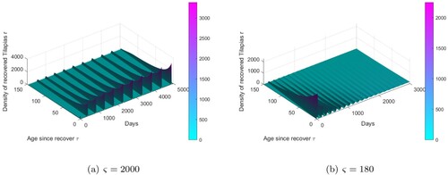
Figure 2. In 3D figures (a,b), we present the density of recovered tilapias. (a) $\varsigma =2000$. (b) $\varsigma =180$.

5. Discussion and conclusion

This work concerns a model of TiLV occurring in tilapia's populations. Because understanding the role of the adaptive immune response following exposure of tilapia to TiLV is a critical step in the development of a vaccine [33], our model incorporates the rate at which recovered individuals lose their immunity. We have established a mathematical well-posedness result obtained by mean of integrated semi-group theory, have computed the basic reproduction number and proved the stability of the disease-free equilibrium. Finally, we have performed some numerical simulations to prove the existence of the endemic equilibrium, the persistence of the disease and to illustrate the role of waning on the epidemic evolution.

The form of ${\mathcal{R}}_0$ given in (15(15) $\begin{array}{r}{\mathcal{R}}_0={\mathcal{R}}_0^{Hdir}+{\mathcal{R}}_0^{Hind}+{\mathcal{R}}_0^V,\end{array}$(15) ) has a biological meaning; indeed ${\mathcal{R}}_0$ depicts the expected number of secondary infections resulting from a single primary infection into an otherwise susceptible population. The term ${\mathcal{R}}_0^{Hdir}$ is the average number of secondary infections produced by one infective individual during its infectious period by horizontal direct transmission while ${\mathcal{R}}_0^{Hind}$ represents the average number of secondary infections produced by one infective individual during its infectious period by horizontal indirect transmission. ${\mathcal{R}}_0^V$ is the average number of secondary infections produced by one infective individual during its infectious period by Vertical transmission. Our study showed the possibility of several outcomes depending on the basic reproduction number ${\mathcal{R}}_0$, which led us to find mathematically the existence and the local stability of the disease-free equilibrium when, ${\mathcal{R}}_0<1$. Then, using numerical simulations, we found the existence of a unique endemic equilibrium for the system (1(1) $\begin{array}{r}\{\begin{array}{l}{\displaystyle \frac{\mathrm{d}S(t)}{\mathrm{d}t}=(b-J(t)-({\mu }_0+{\mu }_{1}N(t)))S(t)+bR(t)}\\ +b{\int }_0^{\mathrm{\infty }}(1-\pi (a))i(a,t)\mathrm{d}a+{\int }_0^{\mathrm{\infty }}\gamma (\tau )r(\tau ,t)\mathrm{d}\tau ,\\ {\displaystyle \frac{\mathrm{\partial }i(a,t)}{\mathrm{\partial }t}+\frac{\mathrm{\partial }i(a,t)}{\mathrm{\partial }a}=-(\delta (a)+{\mu }_i(a)+{\mu }_0+{\mu }_{1}N(t))i(a,t),}\\ {\displaystyle \frac{\mathrm{\partial }r(\tau ,t)}{\mathrm{\partial }t}+\frac{\mathrm{\partial }r(\tau ,t)}{\mathrm{\partial }\tau }=-(\gamma (\tau )+{\mu }_0+{\mu }_{1}N(t))r(\tau ,t),}\\ {\displaystyle \frac{\mathrm{d}V(t)}{\mathrm{d}t}=(1-p){\int }_0^{\mathrm{\infty }}\beta (a)i(a,t)\mathrm{d}a-{\mu }_{V}V(t),}\end{array}\end{array}$(1) )–(4(4) $\begin{array}{r}\begin{array}{l}S(0)=S_0,i(a,0)=i_0(a),r(\tau ,0)=r_0(\tau )\mathrm{and}V(0)=V_0.\end{array}\end{array}$(4) ), and the persistence of the disease in the population, when ${\mathcal{R}}_0>1$.

In order to have a better insight of the influence of waning on the dynamics of the model, we performed numerical simulation with waning parameter $\gamma (.)$ that varies with respect to a bifurcation parameter ς. The results of these simulations in both cases suggest that endemic equilibrium may lose its stability via a Hopf bifurcation, thus giving rise to stable periodic solutions. Biologically, this means that when the temporary immunity period is within a certain range, there will be periodic outbreaks of epidemic, and the disease will not be eradicated from the population [6]. When the bifurcation parameter $\varsigma =180,$ then the mean time to loss immunity is $\tilde{T}\approx 90$ days and the period of the oscillations increases monotonically with time, while the amplitude decreases with time and converges to an endemic equilibrium, see Figures 1(b ,d,f) and 2(b). When the bifurcation parameter $\varsigma =2000,$ the mean time to loss immunity is $\tilde{T}\approx 1000$ days and Figures 1(a,c,e) and 2(a) show waves of epidemic, with period and amplitude increasing with time until converging to a periodic solution of period $T\approx 500$ days. It also appears that considering a given period, the cumulative number of infected individuals in the case $\varsigma =180$ is very high when compared with the cumulative number of infected individuals in the case $\varsigma =2000$ (figures not shown). This means that a vaccine or genetic selection of tilapia, aiming to increase the duration of waning will reduce the severity of the disease even if it will not completely eliminate the disease in the population. In both cases, the value of the basic reproduction number ${\mathcal{R}}_0$ remains unchanged. This is explained by the fact that the expression of ${\mathcal{R}}_0$ does not depend on the waning rate $\gamma (\cdot ).$

In contrast to the model developed in [19], the present model:

• is able to reproduce all the scenarios developed in [19], namely the role of routes of transmissions of the TiLV. Therefore, it extends the model developed in [19].

• is able to study the influence of waning on the dynamics of transmissions of the TiLV, in particular, the waning plays a crucial role on the kinetics and the level of endemicity of disease propagation because the loss of immunity creates another time delay that can destabilize dynamics as shown in [2]:

  • when the temporary immunity period is within a certain range (about 1000 days), there will be periodic outbreaks of epidemic, and the disease will not be eradicated from the population, see on Figures 1(a,c,e) and 2(a) as shown in [6].

  • when the temporary immunity period is about 90 days, there are some oscillations on the patterns, see on Figures 1(b,d,f) and 2(b). The existence of those oscillations was also obtained in [19], but their causes were unknown compared to the current model.

• we observe that even if the basic reproductive number ${\mathcal{R}}_0$ of both models are very closed (5.2630 and 5.2781), the disease dynamics in both cases are very different.

• presents higher complexity and challenges to existing tools, some interesting results as the global stability of the disease-free equilibrium and the uniform persistence of the disease mathematically established in [19] were obtained here through numerical simulations.

The model developed in this paper relates to earlier work on modelling diseases with immunity. For example, Gomes et al. [16] have analysed several ODE models with temporary and partial immunity, as well as vaccination, where immunity wanes at a constant rate. They have shown that when a basic reproduction number exceeds unity, the solutions either decay linearly to an endemic steady state, or approach it in an oscillatory manner. In their findings, the immunity waning rate plays an important role in the time scale for oscillatory behaviour. While our model also highlights the importance of the waning and shows oscillatory behaviours of period depending on the waning rate. Since, temporary immunity is likely to wane at an increasing rate, we assumed that the duration of the immunity loss decays linearly with time since recovery. This led us to a simple form of the rate $\gamma (\tau )$. However, with more biological data, one could adopt more complicated forms of the waning rate as in [5]. Indeed, in reality, the immune system of individuals may be boosted through exposition to the disease. This feature is a factor considered in several existing models through the immunity clock, that is by resetting the recovery age [27] or through the inclusion of additional internal states (within-host dynamics), see for instance [15,17].

Acknowledgments

The authors are very grateful to the editors and the anonymous referees for their valuable comments and suggestions, which helped us to improve significantly the presentation of this work.

Disclosure statement

No potential conflict of interest was reported by the author(s).

Additional information

Funding

This work was funded by a grant from the African Institute for Mathematical Sciences, www.nexteinstein.org, with financial support from the Government of Canada, provided through Global Affairs Canada, www.international.gc.ca, and the International Development Research Centre, www.idrc.ca.

References

- S.K.K. Amponsah, B. Asiedu, and P. Failler, Population parameters of oreochromis niloticus (l) from a semi-open lagoon (Sakumo II), Ghana and its implications on management, Egyptian J. Aquat. Biol. Fish. 24(2) (2020), pp. 195–207.
- E. Bacharach, N. Mishra, T. Briese, M. C. Zody, J. E. Kembou Tsofack, R. Zamostiano, A. Berkowitz, J. Ng, A. Nitido, A. Corvelo, N. C. Toussaint, S. C. Abel Nielsen, M. Hornig, J. Del Pozo, T. Bloom, H. Ferguson, A. Eldar, W. I. Lipkin, C. A. Biron, E. Holmes, and C. Calisher, Characterization of a novel orthomyxo-like virus causing mass die-offs of tilapia, MBio 7(2) (2016), pp. 5561.
- C. Beaumont, J.-B. Burie, A. Ducrot, and P. Zongo, Propagation of Salmonella within an industrial hen house, SIAM J. Appl. Math. 72(4) (2012), pp. 1113–1148.
- B.K. Behera, P.K. Pradhan, T.R. Swaminathan, N. Sood, P. Paria, A. Das, D.K. Verma, R. Kumar, M.K. Yadav, A.K. Dev, P.K. Parida, B.K. Das, K.K. Lal, and J.K. Jena, Emergence of tilapia lake virus associated with mortalities of farmed Nile tilapia Oreochromis niloticus (Linnaeus 1758) in India, Aquaculture 484 (2018), pp. 168–174.
- S. Bhattacharya and F.R. Adler, A time since recovery model with varying rates of loss of immunity, Bullet. Math. Biol. 74(12) (2012), pp. 2810–2819.
- K.B. Blyuss and Y.N. Kyrychko, Stability and bifurcations in an epidemic model with varying immunity period, Bullet. Math. Biol. 72(2) (2010), pp. 490–505.
- F. Brauer, Z. Shuai, and P. van den Driessche, Dynamics of an age-of-infection cholera model, Math. Biosci. Eng. 10(5–6) (2013), pp. 1335–1349.
- Y. Cai, Y. Kang, M. Banerjee, and W. Wang, Complex dynamics of a host-parasite model with both horizontal and vertical transmissions in a spatial heterogeneous environment, Nonlinear Anal.: Real World Appl. 40 (2018), pp. 444–465.
- S.B. Chakraborty and B. Samir, Comparative growth performance of mixed-sex and monosex Nile tilapia at various stocking densities during cage culture, Recent Res. Sci. Technol. 4(11) (2012), pp. 46–50.
- N. Dinh-Hung, P. Sangpo, T. Kruangkum, P. Kayansamruaj, T. Rung-ruangkijkrai, S. Senapin, C.Rodkhum, and H.T. Dong, Dissecting the localization of tilapia tilapinevirus in the brain of the experimentally infected Nile tilapia, Oreochromis niloticus (l.), J. Fish Dis. 44(8) (2021), pp. 1053–1064.
- H.T. Dong, S. Senapin, W. Gangnonngiw, V.V. Nguyen, C. Rodkhum, P.P. Debnath, J.Delamare-Deboutteville, and C.V. Mohan, Experimental infection reveals transmission of tilapia lake virus (tilv) from tilapia broodstock to their reproductive organs and fertilized eggs, Aquaculture 515 (2020), pp. 734541.
- H.T. Dong, S. Siriroob, W. Meemetta, W. Santimanawong, W. Gangnonngiw, N. Pirarat, P. Khunrae, T. Rattanarojpong, R. Vanichviriyakit, and S. Senapin, Emergence of tilapia lake virus in Thailand and an alternative semi-nested rt-pcr for detection, Aquaculture 476 (2017), pp. 111–118.
- M. Eyngor, R. Zamostiano, J.E. Kembou Tsofack, A. Berkowitz, H. Bercovier, S. Tinman, M. Lev, A.Hurvitz, M. Galeotti, E. Bacharach, and A. Eldar, Identification of a novel RNA virus lethal to tilapia, J. Clin. Microbiol. 52(12) (2014), pp. 4137–4146.
- M. Firdaus-Nawi and M. Zamri-Saad, Major components of fish immunity: A review, Pertanika J. Trop. Agric. Sci. 39(4) (2016), pp. 393–420.
- A. Gandolfi, A. Pugliese, and C. Sinisgalli, Epidemic dynamics and host immune response: A nested approach, J. Math. Biol. 70(3) (2015), pp. 399–435.
- M.G.M. Gomes, L.J. White, and G.F. Medley, Infection, reinfection, and vaccination under suboptimal immune protection: Epidemiological perspectives, J. Theor. Biol. 228(4) (2004), pp. 539–549.
- H. Gulbudak, V.L. Cannataro, N. Tuncer, and M. Martcheva, Vector-borne pathogen and host evolution in a structured immuno-epidemiological system, Bullet. Math. Biol. 79(2) (2017), pp. 325–355.
- A. Ivan, Z. Thaddeus, I. Andrew, N. K. Howard, M. Norman, B. Steven, N. Mujibu, D. B. Sylvester, L. N. H. David, and E. Jackson, Effect of stocking density on growth and survival of Nile tilapia (Oreochromis niloticus, Linnaeus 1758) under cage culture in Lake Albert, Uganda, Int. J. Fish. Aquac.12(2) (2020), pp. 26–35.
- C. Kenne, R. Dorville, G. Mophou, and P. Zongo, An age-structured model for tilapia lake virus transmission in freshwater with vertical and horizontal transmission, Bullet. Math. Biol. 83(90) (2021), pp. 1–35.
- G.W. Litman, J.P. Rast, and S.D. Fugmann, The origins of vertebrate adaptive immunity, Nat. Rev. Immunol. 10(8) (2010), pp. 543–553.
- P. Magal, C.C. McCluskey, and G.F. Webb, Lyapunov functional and global asymptotic stability for an infection-age model, Appl. Anal. 89(7) (2010), pp. 1109–1140.
- P. Magal, O. Seydi, and F.-B. Wang, Monotone abstract non-densely defined Cauchy problems applied to age structured population dynamic models, J. Math. Anal. Appl. 479(1) (2019), pp. 450–481.
- B. Magnadóttir, Innate immunity of fish (overview), Fish Shellfish Immunol. 20(2) (2006), pp. 137–151.
- M. Martcheva and H.R. Thieme, Progression age enhanced backward bifurcation in an epidemic model with super-infection, J. Math. Biol. 46(5) (2003), pp. 385–424.
- K.K. Mugimba, M. Lamkhannat, S. Dubey, S. Mutoloki, H.M. Munangandu, and O. Evensen, Tilapia lake virus downplays innate immune responses during early stage of infection in Nile tilapia (Oreochromis niloticus), Scientific Reports 10(1) (2020), pp. 1–12.
- R.A. Myers, K.G. Bowen, and N.J. Barrowman, Maximum reproductive rate of fish at low population sizes, Canadian Journal of Fisheries and Aquatic Sciences 56(12) (1999), pp. 2404–2419.
- K. Okuwa, H. Inaba, and T. Kuniya, An age-structured epidemic model with boosting and waning of immune status, Math. Biosci. Eng. 18(5) (2021), pp. 5707–5736.
- D. Pokorova, T. Vesely, V. Piackova, S. Reschova, and J. Hulova, Current knowledge on koi herpesvirus (khv): a review, Vet. Med. Czech 50(4) (2005), pp. 139–148.
- M. Rafiq I. Sarder, K.D. Thompson, D.J. Penman, and B.J. McAndrew, Immune responses of Nile tilapia (Oreochromis niloticus l.) clones: I. Non-specific responses, Developmental
- Q. Richard, M. Choisy, T. Lefèvre, and R. Djidjou-Demasse, Human-vector malaria transmission model structured by age, time since infection and waning immunity, Nonlinear Analysis: Real World Applications 63 (2022), pp. 103393.
- M. Rubio-Godoy, Teleost fish immunology. review, Revista Mexicana De Ciencias Pecuarias 1(1) (2010), pp. 47–57.
- T. Shimizu, N. Yoshida, H. Kasai, and M. Yoshimizu, Survival of koi herpesvirus (khv) in environmental water, Fish Pathology 41(4) (2006), pp. 153–157.
- P. Tattiyapong, W. Dechavichitlead, T.B. Waltzek, and W. Surachetpong, Tilapia develop protective immunity including a humoral response following exposure to tilapia lake virus, Fish & Shellfish Immunology 106 (2020), pp. 666–674.
- C. Uribe, H. Folch, R. Enríquez, and G.J.V.M. Moran, Innate and adaptive immunity in teleost fish: A review, Veterinarni Medicina 56(10) (2011), pp. 486–503.
- J. Yamkasem, P. Tattiyapong, A. Kamlangdee, and W. Surachetpong, Evidence of potential vertical transmission of tilapia lake virus, J. Fish Dis. 42(9) (2019), pp. 1293–1300.
- Y.-F. Yang, T.-H. Lu, H.-C. Lin, C.-Y. Chen, and C. Liao, Assessing the population transmission dynamics of tilapia lake virus in farmed tilapia, J. Fish Dis. 419 (2018), pp. 1439–1448.
- J. Yang, Z. Qiu, and X.-Z. Li, Global stability of an age-structured cholera model, Math. Biosci. Eng.11(3) (2014), pp. 641–665.
- E. Yongo and N. Outa, Growth and population parameters of Nile tilapia, Oreochromis niloticus (L.) in the open waters of Lake Victoria, Kenya, Lakes & Reservoirs: Research & Management 21(4) (2016), pp. 375–379.
- W. Zeng, Y. Wang, X. Chen, Q. Wang, S.M. Bergmann, Y. Yang, Y. Wang, B. Li, Y. Lv, H. Li, and W.Lan, Potency and efficacy of vp20-based vaccine against tilapia lake virus using different prime-boost vaccination regimens in tilapia, Aquaculture 539 (2021), pp. 736654.