Uniqueness and stability of periodic solutions for an interactive wild and Wolbachia-infected male mosquito model

Abstract

We investigate a mosquito population suppression model, which includes the release of Wolbachia-infected males causing incomplete cytoplasmic incompatibility (CI). The model consists of two sub-equations by considering the density-dependent birth rate of wild mosquitoes. By assuming the release waiting period T is larger than the sexual lifespan $\overline{T}$ of Wolbachia-infected males, we derive four thresholds: the CI intensity threshold $s_h^{\ast }$, the release amount thresholds $g^{\ast }$ and $c^{\ast }$, and the waiting period threshold $T^{\ast }$. From a biological view, we assume $s_h>s_h^{\ast }$ throughout the paper. When $g^{\ast }<c<c^{\ast }$, we prove the origin $E_0$ is locally asymptotically stable iff $T<T^{\ast }$, and the model admits a unique T-periodic solution iff $T\ge T^{\ast }$, which is globally asymptotically stable. When $c\ge c^{\ast }$, we show the origin $E_0$ is globally asymptotically stable iff $T\le T^{\ast }$, and the model has a unique T-periodic solution iff $T>T^{\ast }$, which is globally asymptotically stable. Our theoretical results are confirmed by numerical simulations.

Keywords:

• Mosquito population suppression
• Wolbachia
• incomplete CI
• periodic solutions
• uniqueness
• global asymptotic stability

1. Introduction

Mosquitoes can spread diseases between humans, or from animals to humans. They ingest pathogens from an infected host and then transmit diseases during subsequent bites. Common mosquito-borne diseases include dengue, chikungunya, Zika, etc. [37]. The World Health Organization has reported that an estimated 100–400 million people are infected with dengue each year [38]. In recent years, dengue has spread rapidly in more than 129 countries [3]. Traditional ways to prevent the transmission of dengue are integrated mosquito management which includes spraying insecticide or removing breeding sites [1,36]. However, besides environmental pollution, spraying insecticide has only a short-term effect on eradicating mosquitoes due to the emergence of insecticide resistance [32,34]. At the same time, removing all breeding sites of larva mosquitoes is an impossible mission. Although the dengue vaccine Dengvaxia was approved for use in 2015, the safety of the vaccine cannot be guaranteed due to the phenomenon of antibody-dependent enhancement [9,11].

Nowadays, an innovative biological control strategy involves an intracellular bacterium called Wolbachia, which exists in about 20% arthropod hosts [19,35]. Wolbachia was first identified in 1924 by Hertig and Wolbach, and has gained widespread attention of researchers after its role in cytoplasmic incompatibility (CI) was revealed by Laven [21] in 1956. CI occurs when Wolbachia-infected males mate with Wolbachia-uninfected females, resulting in eggs produced from mated females will not hatch [15,29]. Since then, scientists have made great efforts to inject Wolbachia into Aedes mosquitoes to offer possible biological tools to combat dengue and other mosquito-borne diseases. The groundbreaking work was credited to Xi et al. [39], who successfully established the first stable Wolbachia strain, named as WB1, in Aedes aegypti by embryonic microinjection in 2005. Subsequent experiments showed that WB1 induced complete CI. Owing to this breakthrough, various Wolbachia strains have been stably established in Aedes albopictus [40], which is the sole vector of dengue in Guangzhou. In 2015, Xi's team built the largest mosquito factory of the world in Guangzhou, China, and a three-year field trial in Shazai island and Dadaosha island by releasing factory-reared male mosquitoes eradicated more than 95% of Aedes albopictus mosquito populations [48].

As the successful establishment of various Wolbachia strains in mosquitoes, mathematical modelling and analysing on the interactive dynamics of wild and released mosquitoes has attracted plenty of attention [5–7,22,23,30,33,42,44]. Various mathematical models have been established, including discrete models [4,8,45,47,50], which are suited to cage mosquito populations, ordinary differential equation models [13,20,49] and delay differential equation models [41,43], which consider the overlapping generations in mosquito populations and the maturation delay of mosquitoes from egg to reproductive adults, respectively. Also, stochastic models [16,17] have been developed to include the random switch of environments, and reaction diffusion models [18,28,31] have been investigated to include the effect of mosquito dispersal on the interactive dynamics of wild and released mosquitoes.

Among most of the above models, the authors assumed that CI is complete, i.e. no eggs from the incompatible mating will hatch. Complete CI is the most ideal situation when we aim to sterilize wild females through CI by releasing Wolbachia-infected males. However, experiments showed that CI could be incomplete [10,40] due to different hosts or different Wolbachia strains, which could also be influenced by environmental conditions. In this paper, we aim to develop a mosquito suppression model which includes both the release of male mosquitoes and the incomplete CI mechanism. To this end, we introduce the first parameter $s_h\in (0,1)$ to estimate the CI intensity. That is, $s_h$ is the relative reduction in egg hatch caused by incompatible crosses, and the hatch rate of the compatible case is $s_h=1$. Let $w(t)$ and $g(t)$ be the numbers of wild and Wolbachia-infected mosquitoes at time t, respectively. Then the ratio $g(t)/(w(t)+g(t))$ represents the probability of wild mosquitoes mating with Wolbachia-infected mosquitoes under the assumption of random mating behaviour [8]. Let a be the total number of offspring per wild mosquito per unit time. With the interference of Wolbachia-infected males, the birth rate of wild mosquitoes is reduced from a to $a\cdot (\frac{w(t)}{w(t)+g(t)}+\frac{(1-s_h)g(t)}{w(t)+g(t)})=a\cdot (1-s_h\frac{g(t)}{w(t)+g(t)}).$Meanwhile, mosquitoes go through four stages of complete metamorphosis: egg, pupa, larva, and adult, with the first three stages named as aquatic stages. Based on the experimental observations that the crowding effect basically takes place in aquatic stages [12,14], many authors included the density-dependent effect in the growth of the mosquito population [24,26]. Under this consideration, we also assume that the density dependence (denoted by ξ) of mosquitoes development process takes place in aquatic stages. Thus, the birth rate of wild mosquitoes is $a\cdot (1-s_h\frac{g(t)}{w(t)+g(t)})\cdot (1-\xi (w(t)+g(t))).$Together with the assumption that the death rate of wild mosquitoes is density-independent, we reach the following model, (1) $\frac{\mathrm{d}w(t)}{\mathrm{d}t}=a(1-s_h\frac{g(t)}{w(t)+g(t)})(1-\xi (w(t)+g(t)))w(t)-\mu w(t),$(1) where μ is the death rate of wild mosquitoes, and we assume that $a>\mu$.

We should mention here that the modelling idea in our model which treated the released male mosquitoes as a given function $g(t)$ was first proposed by Yu [41]. In [41], Yu developed an effective strategy to suppress wild mosquitoes by releasing Wolbachia-infected male mosquitoes, which is governed by a given function $g(t)$. This strategy reduces the difficulties in theoretical researches by reducing dimensions of systems. Since then, this novel modelling idea has attracted a great attention of many scholars. Yu introduced a parameter $\overline{T}$ as the sexual activity lifespan of Wolbachia-infected males. The release function $g(t)$ is then determined by the relation of $\overline{T}$ with the waiting period T between two consecutive releases. We assume that the Wolbachia-infected mosquitoes are released impulsively and periodically at discrete time points $T_k=kT,k=0,1,2,\dots$, and the release amount of each batch is maintained at a constant level c. The simplest case of $g(t)$ happens when $T=\overline{T}$, that is, once the released males lose their mating ability, another batch of infected males is released supplementarily. Thus, we have the release function $g(t)\equiv c,\mathrm{for}T=\overline{T},$and Model (1(1) $\frac{\mathrm{d}w(t)}{\mathrm{d}t}=a(1-s_h\frac{g(t)}{w(t)+g(t)})(1-\xi (w(t)+g(t)))w(t)-\mu w(t),$(1) ) takes the form (2) $\frac{\mathrm{d}w(t)}{\mathrm{d}t}=a(1-s_h\frac{c}{w(t)+c})(1-\xi (w(t)+c))w(t)-\mu w(t).$(2) We provide a complete dynamics of Model (2(2) $\frac{\mathrm{d}w(t)}{\mathrm{d}t}=a(1-s_h\frac{c}{w(t)+c})(1-\xi (w(t)+c))w(t)-\mu w(t).$(2) ) in Section 2, which is the basis for the discussion of $T>\overline{T}$ and $T<\overline{T}$. We only focus on the case $T>\overline{T}$ in this paper and leave the case $T<\overline{T}$ in future work. Thus, the release function $g(t)$ becomes $g(t)=\{\begin{array}{ll}c,& \mathrm{for}t\in [iT,iT+\overline{T}),\\ 0,& \mathrm{for}t\in [iT+\overline{T},(i+1)T),\end{array}i=0,1,2,\dots ,$and Model (1(1) $\frac{\mathrm{d}w(t)}{\mathrm{d}t}=a(1-s_h\frac{g(t)}{w(t)+g(t)})(1-\xi (w(t)+g(t)))w(t)-\mu w(t),$(1) ) can be rewritten as two sub-equations (3) $\begin{array}{rl}\frac{\mathrm{d}w}{\mathrm{d}t}& =a(1-s_h\frac{c}{w+c})(1-\xi (w+c))w-\mu w,\mathrm{for}t\in [iT,iT+\overline{T}),i=0,1,2,\dots ,\end{array}$(3) (4) $\begin{array}{rl}\frac{\mathrm{d}w}{\mathrm{d}t}& =-a\xi w(w-A),\mathrm{for}t\in [iT+\overline{T},(i+1)T),i=0,1,2,\dots ,\end{array}$(4) where $A=(a-\mu )/a\xi$.

In this study, we formulate a mosquito population suppression model interfered by Wolbachia-infected males causing incomplete CI. In Section 2, the local and global dynamics of wild mosquitoes are studied completely when $T=\overline{T}$. In Section 3, by using Poincaré map, we obtain the sufficient and necessary conditions for the stability of the origin $E_0$ and the existence and uniqueness of a globally asymptotically stable T-periodic solution for the case $T>\overline{T}$, respectively. Finally, some numerical examples are provided to confirm our main results in Section 4.

2. The dynamical behaviour for the case $T=\overline{T}$

In this section, we focus on a special release strategy, that is, the waiting period T between two consecutive releases is equal to the sexual activity lifespan $\overline{T}$. The release amount of each batch is controlled at stable level c, and the loss of released mosquitoes during the short sexual activity lifespan can be ignored. Thus, the total amount of released mosquitoes with sexual activity is maintained at the level c. The dynamics of wild mosquitoes $\omega (t)$ are mainly governed by (2(2) $\frac{\mathrm{d}w(t)}{\mathrm{d}t}=a(1-s_h\frac{c}{w(t)+c})(1-\xi (w(t)+c))w(t)-\mu w(t).$(2) ). Thus, to better understand the dynamical behaviours, we need to count the positive equilibria of (2(2) $\frac{\mathrm{d}w(t)}{\mathrm{d}t}=a(1-s_h\frac{c}{w(t)+c})(1-\xi (w(t)+c))w(t)-\mu w(t).$(2) ) and analyse their stability.

We claim that Model (2(2) $\frac{\mathrm{d}w(t)}{\mathrm{d}t}=a(1-s_h\frac{c}{w(t)+c})(1-\xi (w(t)+c))w(t)-\mu w(t).$(2) ) has no positive equilibrium when the release amount $c\ge 1/\xi$. In fact, from (2(2) $\frac{\mathrm{d}w(t)}{\mathrm{d}t}=a(1-s_h\frac{c}{w(t)+c})(1-\xi (w(t)+c))w(t)-\mu w(t).$(2) ) we easy to find that the part in the first bracket is positive and the part in the second bracket is negative when $c\ge 1/\xi$. Taking together, we derive that the right part of (2(2) $\frac{\mathrm{d}w(t)}{\mathrm{d}t}=a(1-s_h\frac{c}{w(t)+c})(1-\xi (w(t)+c))w(t)-\mu w(t).$(2) ) is negative for all $\omega (t)>0$ implying that (2(2) $\frac{\mathrm{d}w(t)}{\mathrm{d}t}=a(1-s_h\frac{c}{w(t)+c})(1-\xi (w(t)+c))w(t)-\mu w(t).$(2) ) has no positive equilibrium. In the following, we only need to consider the case that $0<c<1/\xi$ and analyse the existence of the positive equilibria over the rectangular area in $s_h$-c plane, as shown in Figure 1. We rewrite (2(2) $\frac{\mathrm{d}w(t)}{\mathrm{d}t}=a(1-s_h\frac{c}{w(t)+c})(1-\xi (w(t)+c))w(t)-\mu w(t).$(2) ) as (5) $\{\begin{array}{l}{\displaystyle \frac{\mathrm{d}w}{\mathrm{d}t}}={\displaystyle \frac{-wf(w)}{w+c}},\\ w(0)=u,\end{array}$(5) where $f(w)=a\xi w^2+(a\xi c(2-s_h)-(a-\mu ))w+c(\mu -a(1-s_h)(1-\xi c)).$ The equilibria of Model (5(5) $\{\begin{array}{l}{\displaystyle \frac{\mathrm{d}w}{\mathrm{d}t}}={\displaystyle \frac{-wf(w)}{w+c}},\\ w(0)=u,\end{array}$(5) ) satisfy $-wf(w)/(w+c)=0$. It is very obvious that Model (5(5) $\{\begin{array}{l}{\displaystyle \frac{\mathrm{d}w}{\mathrm{d}t}}={\displaystyle \frac{-wf(w)}{w+c}},\\ w(0)=u,\end{array}$(5) ) has at least one trivial equilibrium $E_0=0$. We then search other equilibria from $f(w)=0$. Since $f(w)=0$ is a quadratic equation, its discriminant is $\mathrm{\Delta }=a^2{\xi }^2{s}_h^2{c}^2-2a\xi s_h(a+\mu )c+(a-\mu {)}^2,$which is a quadratic polynomial with respect to c. It is easy to find that there are two positive real roots $c_1$ and $c_2$ such that $\mathrm{\Delta }=0$, where $c_1$ and $c_2$ are given as $c_1=\frac{a+\mu -2\sqrt{a\mu }}{a\xi s_h}\mathrm{and}{c}_2=\frac{a+\mu +2\sqrt{a\mu }}{a\xi s_h}.$The two roots divide $(0,\mathrm{\infty })$ into three intervals: $(0,c_1],(c_1,c_2)$ and $[c_2,\mathrm{\infty })$. We compare $c_2$ with $1/\xi$ and find $c_2-\frac{1}{\xi }=\frac{a(1-s_h)+\mu +2\sqrt{a\mu }}{a\xi s_h}>0,$which implies that Model (5(5) $\{\begin{array}{l}{\displaystyle \frac{\mathrm{d}w}{\mathrm{d}t}}={\displaystyle \frac{-wf(w)}{w+c}},\\ w(0)=u,\end{array}$(5) ) has no positive equilibrium when the release amount $c\in [c_2,\mathrm{\infty })$. When $c\in (c_1,c_2)$, the discriminant $\mathrm{\Delta }<0$ holds, then $f(w)$ is positive for all w>0, thus Model (5(5) $\{\begin{array}{l}{\displaystyle \frac{\mathrm{d}w}{\mathrm{d}t}}={\displaystyle \frac{-wf(w)}{w+c}},\\ w(0)=u,\end{array}$(5) ) also has no positive equilibrium.

Figure 1. The distribution of positive equilibria N in Model (5(5) $\{\begin{array}{l}{\displaystyle \frac{\mathrm{d}w}{\mathrm{d}t}}={\displaystyle \frac{-wf(w)}{w+c}},\\ w(0)=u,\end{array}$(5) ).

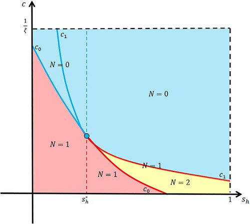
We only need to find the positive equilibria for $c\in (0,c_1]$. When $c=c_1$, we have $\mathrm{\Delta }=0$ and derive a unique equilibrium of (5(5) $\{\begin{array}{l}{\displaystyle \frac{\mathrm{d}w}{\mathrm{d}t}}={\displaystyle \frac{-wf(w)}{w+c}},\\ w(0)=u,\end{array}$(5) ), that is, $E^{\ast }=\frac{a-\mu -a\xi c_1(2-s_h)}{2a\xi }.$From the expression of $c_1$, it is a function of $s_h$ when $s_h$ varies over $(0,1)$. This curve divides the rectangle in Figure 1 into two areas. For the case that the release amount $c=c_1$, the equilibrium $E^{\ast }$ is positive only when $s_h>s_h^{\ast }$, where (6) $s_h^{\ast }=\frac{a-\sqrt{a\mu }}{a}.$(6) When $c\in (0,c_1)$, Model (5(5) $\{\begin{array}{l}{\displaystyle \frac{\mathrm{d}w}{\mathrm{d}t}}={\displaystyle \frac{-wf(w)}{w+c}},\\ w(0)=u,\end{array}$(5) ) has two equilibria, that is, $E_1=\frac{a-\mu -a\xi c(2-s_h)-\sqrt{\mathrm{\Delta }}}{2a\xi }\mathrm{and}{E}_2=\frac{a-\mu -a\xi c(2-s_h)+\sqrt{\mathrm{\Delta }}}{2a\xi }.$Now, we need to determine the signs of the two equilibria. Since $f(w)$ is a convex function, it is easy to get that $f(w)=0$ has a unique positive root when $f(0)<0$, or $f(0)=0$ and $a\xi c(2-s_h)-a+\mu >0$. We consider $f(0)=0$ and derive another curve $c_0=\frac{a(1-s_h)-\mu }{a\xi (1-s_h)},\mathrm{for}{s}_h\in (0,\frac{a-\mu }{a}],$which is tangent to $c_1$ at $s_h^{\ast }$. The two curves divide the rectangle in Figure 1 into six areas. When $c<c_0$, we have $f(0)<0$ and Model (5(5) $\{\begin{array}{l}{\displaystyle \frac{\mathrm{d}w}{\mathrm{d}t}}={\displaystyle \frac{-wf(w)}{w+c}},\\ w(0)=u,\end{array}$(5) ) has a unique equilibrium $E_2$. When $c=c_0$, Model (5(5) $\{\begin{array}{l}{\displaystyle \frac{\mathrm{d}w}{\mathrm{d}t}}={\displaystyle \frac{-wf(w)}{w+c}},\\ w(0)=u,\end{array}$(5) ) has a unique positive equilibrium $E_2$ if $s_h>s_h^{\ast }$ and has no positive equilibrium if $s_h\le s_h^{\ast }$. By further analysing, we find $f(0)>0$ when $c>c_0$, and Model (5(5) $\{\begin{array}{l}{\displaystyle \frac{\mathrm{d}w}{\mathrm{d}t}}={\displaystyle \frac{-wf(w)}{w+c}},\\ w(0)=u,\end{array}$(5) ) has two positive equilibria $E_1$ and $E_2$ if $c\in (c_m,c_1)$ and $s_h>s_h^{\ast }$, where $c_m=max\{0,c_0\}$, and has no positive equilibrium if $s_h\le s_h^{\ast }$. Now, we can give the main results as follows.

Theorem 2.1

For the case $s_h\in (0,s_h^{\ast }]$, the following conclusions hold.

1. If $c\in (0,c_0)$, then Model (5(5) $\{\begin{array}{l}{\displaystyle \frac{\mathrm{d}w}{\mathrm{d}t}}={\displaystyle \frac{-wf(w)}{w+c}},\\ w(0)=u,\end{array}$(5) ) has two non-negative equilibria: the origin $E_0$ and the unique positive equilibrium $E_2$, where $E_0$ is unstable and $E_2$ is asymptotically stable.

2. If $c\in [c_0,1/\xi )$, then Model (5(5) $\{\begin{array}{l}{\displaystyle \frac{\mathrm{d}w}{\mathrm{d}t}}={\displaystyle \frac{-wf(w)}{w+c}},\\ w(0)=u,\end{array}$(5) ) has only one non-negative equilibrium $E_0$, and $E_0$ is globally asymptotically stable.

Theorem 2.2

For the case $s_h\in (s_h^{\ast },1)$, the following conclusions hold.

1. If $c\in (0,c_0]$, then Model (5(5) $\{\begin{array}{l}{\displaystyle \frac{\mathrm{d}w}{\mathrm{d}t}}={\displaystyle \frac{-wf(w)}{w+c}},\\ w(0)=u,\end{array}$(5) ) has two non-negative equilibria: the origin $E_0$ and the unique positive equilibrium $E_2$, where $E_0$ is unstable and $E_2$ is asymptotically stable.

2. If $c\in (c_m,c_1)$, then Model (5(5) $\{\begin{array}{l}{\displaystyle \frac{\mathrm{d}w}{\mathrm{d}t}}={\displaystyle \frac{-wf(w)}{w+c}},\\ w(0)=u,\end{array}$(5) ) has three non-negative equilibria: the origin $E_0$, two positive equilibria $E_1$ and $E_2$, where both $E_0$ and $E_2$ are asymptotically stable, and $E_1$ is unstable.

3. If $c=c_1$, then Model (5(5) $\{\begin{array}{l}{\displaystyle \frac{\mathrm{d}w}{\mathrm{d}t}}={\displaystyle \frac{-wf(w)}{w+c}},\\ w(0)=u,\end{array}$(5) ) has two non-negative equilibria: the origin $E_0$ and the unique positive equilibrium $E^{\ast }$, where $E_0$ is asymptotically stable and $E^{\ast }$ is semi-stable, namely, the right-side of $E^{\ast }$ is stable and the left-side is not.

4. If $c\in (c_1,1/\xi )$, then Model (5(5) $\{\begin{array}{l}{\displaystyle \frac{\mathrm{d}w}{\mathrm{d}t}}={\displaystyle \frac{-wf(w)}{w+c}},\\ w(0)=u,\end{array}$(5) ) has only one equilibrium $E_0$, and $E_0$ is globally asymptotically stable.

Proof.

The existence of equilibria in each domain can be derived from the above analysis, and we only need to prove the stability. We consider the most complicated case, that is, $s_h\in (s_h^{\ast },1)$ and $c\in (c_m,c_1)$. In this case, Model (5(5) $\{\begin{array}{l}{\displaystyle \frac{\mathrm{d}w}{\mathrm{d}t}}={\displaystyle \frac{-wf(w)}{w+c}},\\ w(0)=u,\end{array}$(5) ) has three non-negative equilibria $E_0$, $E_1$ and $E_2$, hence (5(5) $\{\begin{array}{l}{\displaystyle \frac{\mathrm{d}w}{\mathrm{d}t}}={\displaystyle \frac{-wf(w)}{w+c}},\\ w(0)=u,\end{array}$(5) ) can be rewritten as (7) $\frac{\mathrm{d}w}{\mathrm{d}t}=\frac{-a\xi w(w-E_1)(w-E_2)}{w+c}.$(7) The interval $(0,\mathrm{\infty })$ is divided into three intervals: $(0,E_1]$, $(E_1,E_2]$ and $(E_2,\mathrm{\infty })$. From (7(7) $\frac{\mathrm{d}w}{\mathrm{d}t}=\frac{-a\xi w(w-E_1)(w-E_2)}{w+c}.$(7) ), we have $\begin{array}{rl}& \frac{\mathrm{d}w}{\mathrm{d}t}<0,\mathrm{for}u\in (0,E_1),\\ & \frac{\mathrm{d}w}{\mathrm{d}t}>0,\mathrm{for}u\in (E_1,E_2),\\ & \frac{\mathrm{d}w}{\mathrm{d}t}<0,\mathrm{for}u\in (E_2,\mathrm{\infty }),\end{array}$which implies that $E_0$ and $E_2$ are asymptotically stable, and $E_1$ is unstable. The proof of Theorem 2.2(2) is completed. For other cases, the proof is similar and omitted here.

Furthermore, combining Theorems 2.1 and 2.2, we can obtain the CI intensity threshold $s_h^{\ast }$ and the release amount threshold (see Figure 1), (8) $g^{\ast }=\{\begin{array}{ll}{c}_0,& \mathrm{if}{s}_h\in (0,s_h^{\ast }],\\ c_1,& \mathrm{if}{s}_h\in (s_h^{\ast },1).\end{array}$(8) In fact, what we most like to see is that $E_0$ is globally asymptotically stable, which means that no matter what the initial number of wild mosquitoes is, the population will be eventually eradicated in real life. The above theorems state that wild mosquitoes will tend to be extinct when the release amount of Wolbachia-infected males is larger than $g^{\ast }$, otherwise, the mosquito population can only be suppressed locally.

On this basis, we continue to study the case $T>\overline{T}$. When $T>\overline{T}$ and $c>g^{\ast }$, the global dynamics behaviour of Model (1(1) $\frac{\mathrm{d}w(t)}{\mathrm{d}t}=a(1-s_h\frac{g(t)}{w(t)+g(t)})(1-\xi (w(t)+g(t)))w(t)-\mu w(t),$(1) ) will be quite different from the case $T=\overline{T}$. For biological relevance, we only consider $s_h\in (s_h^{\ast },1)$ in the following.

3. The dynamical behaviour for the case $T>\overline{T}$

Since the release period T is greater than the sexual activity lifespan $\overline{T}$ of Wolbachia-infected males, we easy to find that $g(t)$ is a periodic piecewise function and jumps between two constants c and 0. The release strategy makes the time evolution of $w(t)$ switch between (3(3) $\begin{array}{rl}\frac{\mathrm{d}w}{\mathrm{d}t}& =a(1-s_h\frac{c}{w+c})(1-\xi (w+c))w-\mu w,\mathrm{for}t\in [iT,iT+\overline{T}),i=0,1,2,\dots ,\end{array}$(3) ) and (4(4) $\begin{array}{rl}\frac{\mathrm{d}w}{\mathrm{d}t}& =-a\xi w(w-A),\mathrm{for}t\in [iT+\overline{T},(i+1)T),i=0,1,2,\dots ,\end{array}$(4) ). Then Model (1(1) $\frac{\mathrm{d}w(t)}{\mathrm{d}t}=a(1-s_h\frac{g(t)}{w(t)+g(t)})(1-\xi (w(t)+g(t)))w(t)-\mu w(t),$(1) ) has a complex dynamical behaviour.

3.1. The Poincaré map of model (1)

For the case $T>\overline{T}$, the dynamical behaviour of (1(1) $\frac{\mathrm{d}w(t)}{\mathrm{d}t}=a(1-s_h\frac{g(t)}{w(t)+g(t)})(1-\xi (w(t)+g(t)))w(t)-\mu w(t),$(1) ) mainly depends on the constantly switching between (3(3) $\begin{array}{rl}\frac{\mathrm{d}w}{\mathrm{d}t}& =a(1-s_h\frac{c}{w+c})(1-\xi (w+c))w-\mu w,\mathrm{for}t\in [iT,iT+\overline{T}),i=0,1,2,\dots ,\end{array}$(3) ) and (4(4) $\begin{array}{rl}\frac{\mathrm{d}w}{\mathrm{d}t}& =-a\xi w(w-A),\mathrm{for}t\in [iT+\overline{T},(i+1)T),i=0,1,2,\dots ,\end{array}$(4) ). According to (3(3) $\begin{array}{rl}\frac{\mathrm{d}w}{\mathrm{d}t}& =a(1-s_h\frac{c}{w+c})(1-\xi (w+c))w-\mu w,\mathrm{for}t\in [iT,iT+\overline{T}),i=0,1,2,\dots ,\end{array}$(3) ) and (4(4) $\begin{array}{rl}\frac{\mathrm{d}w}{\mathrm{d}t}& =-a\xi w(w-A),\mathrm{for}t\in [iT+\overline{T},(i+1)T),i=0,1,2,\dots ,\end{array}$(4) ), Model (1(1) $\frac{\mathrm{d}w(t)}{\mathrm{d}t}=a(1-s_h\frac{g(t)}{w(t)+g(t)})(1-\xi (w(t)+g(t)))w(t)-\mu w(t),$(1) ) has only one equilibrium $E_0$. Let $w(t)=w(t;0,u)$ be a solution of (1(1) $\frac{\mathrm{d}w(t)}{\mathrm{d}t}=a(1-s_h\frac{g(t)}{w(t)+g(t)})(1-\xi (w(t)+g(t)))w(t)-\mu w(t),$(1) ) with the initial condition $w(0)=u>0$. Clearly, $w(t)$ is continuous and piecewise differentiable. Initial values satisfy $w(0)=u$ on $[0,\overline{T})$ for (3(3) $\begin{array}{rl}\frac{\mathrm{d}w}{\mathrm{d}t}& =a(1-s_h\frac{c}{w+c})(1-\xi (w+c))w-\mu w,\mathrm{for}t\in [iT,iT+\overline{T}),i=0,1,2,\dots ,\end{array}$(3) ) and $w(\overline{T})=w({\overline{T}}^{-})$ on $[\overline{T},T)$ for (4(4) $\begin{array}{rl}\frac{\mathrm{d}w}{\mathrm{d}t}& =-a\xi w(w-A),\mathrm{for}t\in [iT+\overline{T},(i+1)T),i=0,1,2,\dots ,\end{array}$(4) ). In reality, $w(\overline{T};0,u)$ and $w(T;0,u)$ are continuously differentiable with respect to u and $w(\overline{T})$, respectively, where $w(T;0,u)$ can be regarded as a solution of the initial value problem of (4(4) $\begin{array}{rl}\frac{\mathrm{d}w}{\mathrm{d}t}& =-a\xi w(w-A),\mathrm{for}t\in [iT+\overline{T},(i+1)T),i=0,1,2,\dots ,\end{array}$(4) ) with $w(\overline{T})=w({\overline{T}}^{-})$. The solution can be defined in the same way in other intervals. Furthermore, $w(t)=w(t;0,u)$ is a T-periodic solution if $w(T;0,u)=u$. For convenience, we define two continuously differentiable functions $\overline{h}(u)=w(\overline{T};0,u)\mathrm{and}h(u)=w(T;0,u)$throughout this paper.

For Equations (3(3) $\begin{array}{rl}\frac{\mathrm{d}w}{\mathrm{d}t}& =a(1-s_h\frac{c}{w+c})(1-\xi (w+c))w-\mu w,\mathrm{for}t\in [iT,iT+\overline{T}),i=0,1,2,\dots ,\end{array}$(3) ) and (4(4) $\begin{array}{rl}\frac{\mathrm{d}w}{\mathrm{d}t}& =-a\xi w(w-A),\mathrm{for}t\in [iT+\overline{T},(i+1)T),i=0,1,2,\dots ,\end{array}$(4) ), we introduce two new thresholds which are the release amount threshold $c^{\ast }$ and the waiting period threshold $T^{\ast }$, that is, (9) $c^{\ast }=\frac{-a{s}_h+\sqrt{a^2{s}_h^2+4a{s}_h(1-s_h)(a-\mu )}}{2a\xi (1-s_h)},$(9) and (10) $T^{\ast }=\frac{a((\xi c-1)(1-s_h)+1)}{a-\mu }\cdot \overline{T}.$(10) Since $c^{\ast }$ is strictly increasing with respect to $s_h$ and $c^{\ast }=g^{\ast }$ when $s_h=s_h^{\ast }$, we have $c^{\ast }>g^{\ast }$ for $s_h\in (s_h^{\ast },1)$.

Next, we study the initial value problem of Equation (3(3) $\begin{array}{rl}\frac{\mathrm{d}w}{\mathrm{d}t}& =a(1-s_h\frac{c}{w+c})(1-\xi (w+c))w-\mu w,\mathrm{for}t\in [iT,iT+\overline{T}),i=0,1,2,\dots ,\end{array}$(3) ) with $w(0)=u$ on $[0,\overline{T})$ and Equation (4(4) $\begin{array}{rl}\frac{\mathrm{d}w}{\mathrm{d}t}& =-a\xi w(w-A),\mathrm{for}t\in [iT+\overline{T},(i+1)T),i=0,1,2,\dots ,\end{array}$(4) ) with $w(\overline{T})=w({\overline{T}}^{-})$ on $[\overline{T},T)$. We first rewrite (3(3) $\begin{array}{rl}\frac{\mathrm{d}w}{\mathrm{d}t}& =a(1-s_h\frac{c}{w+c})(1-\xi (w+c))w-\mu w,\mathrm{for}t\in [iT,iT+\overline{T}),i=0,1,2,\dots ,\end{array}$(3) ) as (11) $\frac{\mathrm{d}w}{\mathrm{d}t}=-\frac{a\xi w((w-B{)}^2+D^2)}{w+c},$(11) where $B=\frac{A-(2-s_h)c}{2}\mathrm{and}{D}^2=-\frac{a^2{\xi }^2{s}_h^2{c}^2-2a\xi s_h(a+\mu )c+(a-\mu {)}^2}{4a^2{\xi }^2}.$Equation (11(11) $\frac{\mathrm{d}w}{\mathrm{d}t}=-\frac{a\xi w((w-B{)}^2+D^2)}{w+c},$(11) ) is equivalent to $(\frac{\alpha }{w}+\frac{\beta (w-B)}{(w-B{)}^2+D^2}+\frac{\gamma }{(w-B{)}^2+D^2})\mathrm{d}w=-a\xi \mathrm{d}t,$that is, (12) $d(\ln (w^{\alpha }((w-B{)}^2+D^2{)}^{\frac{\beta }{2}}{\mathrm{e}}^{\frac{\gamma }{D}{\tan }^{-1}(\frac{w-B}{D})}))=-a\xi \mathrm{d}t,$(12) where $\begin{array}{rl}& \alpha =\frac{a\xi }{a(1-s_h)(\xi c-1)+\mu },\beta =-\frac{a\xi }{a(1-s_h)(\xi c-1)+\mu },\\ & \gamma =1+\frac{a-\mu -a\xi c(2-s_h)}{2(a(1-s_h)(\xi c-1)+\mu )}.\end{array}$Integrating (12(12) $d(\ln (w^{\alpha }((w-B{)}^2+D^2{)}^{\frac{\beta }{2}}{\mathrm{e}}^{\frac{\gamma }{D}{\tan }^{-1}(\frac{w-B}{D})}))=-a\xi \mathrm{d}t,$(12) ) from 0 to $\overline{T}$, we obtain (13) $\begin{array}{rl}& {\overline{h}}^{\alpha }(u)((\overline{h}(u)-B{)}^2+D^2{)}^{\frac{\beta }{2}}{\mathrm{e}}^{\frac{\gamma }{D}{\tan }^{-1}(\frac{\overline{h}(u)-B}{D})}\\ & =u^{\alpha }((u-B{)}^2+D^2{)}^{\frac{\beta }{2}}{\mathrm{e}}^{\frac{\gamma }{D}{\tan }^{-1}(\frac{u-B}{D})}{\mathrm{e}}^{-a\xi \overline{T}}.\end{array}$(13) We rewrite (4(4) $\begin{array}{rl}\frac{\mathrm{d}w}{\mathrm{d}t}& =-a\xi w(w-A),\mathrm{for}t\in [iT+\overline{T},(i+1)T),i=0,1,2,\dots ,\end{array}$(4) ) as $d(\ln \left(\frac{w}{A-w}\right))=Aa\xi \mathrm{d}t.$Integrating it from $\overline{T}$ to T, we have (14) $\frac{\overline{h}(u)}{A-\overline{h}(u)}=\frac{mh(u)}{A-h(u)},$(14) where $m={\mathrm{e}}^{-Aa\xi (T-\overline{T})}={\mathrm{e}}^{-(a-\mu )(T-\overline{T})}$. Here $h(u)$ is implicitly determined by (13(13) $\begin{array}{rl}& {\overline{h}}^{\alpha }(u)((\overline{h}(u)-B{)}^2+D^2{)}^{\frac{\beta }{2}}{\mathrm{e}}^{\frac{\gamma }{D}{\tan }^{-1}(\frac{\overline{h}(u)-B}{D})}\\ & =u^{\alpha }((u-B{)}^2+D^2{)}^{\frac{\beta }{2}}{\mathrm{e}}^{\frac{\gamma }{D}{\tan }^{-1}(\frac{u-B}{D})}{\mathrm{e}}^{-a\xi \overline{T}}.\end{array}$(13) ) and (14(14) $\frac{\overline{h}(u)}{A-\overline{h}(u)}=\frac{mh(u)}{A-h(u)},$(14) ). Following (13(13) $\begin{array}{rl}& {\overline{h}}^{\alpha }(u)((\overline{h}(u)-B{)}^2+D^2{)}^{\frac{\beta }{2}}{\mathrm{e}}^{\frac{\gamma }{D}{\tan }^{-1}(\frac{\overline{h}(u)-B}{D})}\\ & =u^{\alpha }((u-B{)}^2+D^2{)}^{\frac{\beta }{2}}{\mathrm{e}}^{\frac{\gamma }{D}{\tan }^{-1}(\frac{u-B}{D})}{\mathrm{e}}^{-a\xi \overline{T}}.\end{array}$(13) ) and (14(14) $\frac{\overline{h}(u)}{A-\overline{h}(u)}=\frac{mh(u)}{A-h(u)},$(14) ), we have (15) $\underset{u\to 0}{lim}\frac{\overline{h}(u)}{u}={\mathrm{e}}^{-\frac{a\xi \overline{T}}{\alpha }}\mathrm{and}\underset{u\to 0}{lim}\frac{h(u)}{\overline{h}(u)}=\frac{1}{m}={\mathrm{e}}^{(a-\mu )(T-\overline{T})},$(15) since $\overline{h}(u)\to 0$ and $h(u)\to 0$ as $u\to 0$. Thus, we have (16) $\underset{u\to 0}{lim}\frac{h(u)}{u}=\underset{u\to 0}{lim}(\frac{h(u)}{\overline{h}(u)}\cdot \frac{\overline{h}(u)}{u})={\mathrm{e}}^{(a-\mu )(T-T^{\ast })}.$(16) According to the Poincaré map of Equations (3(3) $\begin{array}{rl}\frac{\mathrm{d}w}{\mathrm{d}t}& =a(1-s_h\frac{c}{w+c})(1-\xi (w+c))w-\mu w,\mathrm{for}t\in [iT,iT+\overline{T}),i=0,1,2,\dots ,\end{array}$(3) ) and (4(4) $\begin{array}{rl}\frac{\mathrm{d}w}{\mathrm{d}t}& =-a\xi w(w-A),\mathrm{for}t\in [iT+\overline{T},(i+1)T),i=0,1,2,\dots ,\end{array}$(4) ), we define two function sequences $\{{\overline{h}}_n(u)\}$ and $\{h_n(u)\}$ by $\{\begin{array}{l}{\overline{h}}_n(u)=w(nT+\overline{T};0,u),\\ h_n(u)=w(nT;0,u),\end{array}n=0,1,2,\dots .$By mathematical induction, we have ${\overline{h}}_0(u)=w(\overline{T};0,u),{\overline{h}}_n(u)=\overline{h}(h_n(u)),n=0,1,2,\dots ,$and (17) $h_0(u)=u,h_{n+1}(u)=w(T;0,h_n(u))=h(h_n(u)),n=0,1,2,\dots .$(17) By using a similar discussion as in [44], we obtain the following lemma.

Lemma 3.1

For any given initial value u>0, the following conclusions hold.

1. If $h(u)>u$, then sequences $\{h_n(u)\}$ and $\{{\overline{h}}_n(u)\}$ are both strictly increasing.

2. If $h(u)=u$, then $h_n(u)\equiv u$. Furthermore, $w(t)=w(t;0,u)$ is a T-periodic solution.

3. If $h(u)<u$, then sequences $\{h_n(u)\}$ and $\{{\overline{h}}_n(u)\}$ are both strictly decreasing.

3.2. Release amount $c\in (g^{\ast },c^{\ast })$

In this case, the release amount c of mosquitoes is controlled between $g^{\ast }$ and $c^{\ast }$. To study the dynamical behaviour, we establish two lemmas before giving the main result.

Lemma 3.2

If $T>T^{\ast }$ and $c>g^{\ast }$ hold, then (1(1) $\frac{\mathrm{d}w(t)}{\mathrm{d}t}=a(1-s_h\frac{g(t)}{w(t)+g(t)})(1-\xi (w(t)+g(t)))w(t)-\mu w(t),$(1) ) has a unique T-periodic solution.

Proof.

First, we show the existence of T-periodic solution. According to (16(16) $\underset{u\to 0}{lim}\frac{h(u)}{u}=\underset{u\to 0}{lim}(\frac{h(u)}{\overline{h}(u)}\cdot \frac{\overline{h}(u)}{u})={\mathrm{e}}^{(a-\mu )(T-T^{\ast })}.$(16) ), we have $\underset{u\to 0}{lim}\frac{h(u)}{u}>1,\mathrm{for}T>T^{\ast }.$Thus, there exists a sufficiently small ${\delta }_0>0$ such that (18) $h(u)>u,\mathrm{for}u\in (0,{\delta }_0).$(18) According to (1(1) $\frac{\mathrm{d}w(t)}{\mathrm{d}t}=a(1-s_h\frac{g(t)}{w(t)+g(t)})(1-\xi (w(t)+g(t)))w(t)-\mu w(t),$(1) ), we know that the solution $w(t)=w(t;0,A)$ is strictly decreasing on $[0,\overline{T})$, that is, we have $\overline{h}(A)<A$, which means that $h(A)<A$ though $w(t)=w(t;0,A)$ is strictly increasing on $[\overline{T},T)$. Hence, there must exist a $u_1\in [{\delta }_0,A)$ such that (19) $h(u_1)=u_1,h^{\prime }(u_1)\le 1,\mathrm{and}h(u)>u,\mathrm{for}u\in (0,u_1).$(19) By Lemma 3.1, we have $w(t;0,u_1)$ is a T-periodic solution of (1(1) $\frac{\mathrm{d}w(t)}{\mathrm{d}t}=a(1-s_h\frac{g(t)}{w(t)+g(t)})(1-\xi (w(t)+g(t)))w(t)-\mu w(t),$(1) ).

Next, the uniqueness of the T-periodic solution is showed by contradiction. Assume that there exists another T-periodic solution $u_2$ in $(u_1,A)$ such that (20) $h(u_2)=u_2,h^{\prime }(u_2)\le 1,\mathrm{and}h(u)<u\mathrm{for}u\in (u_2,A).$(20) Without loss of the generality, we assume that $u_1$ and $u_2$ are the minimal and maximal T-periodic solutions on $[{\delta }_0,A)$, respectively. There must exist a $\overline{v}\in [u_1,u_2]$ such that $h(\overline{v})=\overline{v}$ due to the continuous differentiability of $h(u)$. From the fact that $0<u_1\le \overline{v}\le u_2<A$, there are two cases: $\overline{v}\in (u_1,u_2)$, or $\overline{v}=u_1(\mathrm{or}{u}_2)$.

For the case $\overline{v}\in (u_1,u_2)$, let (21) $P(u)=u^{\alpha }((u-B{)}^2+D^2{)}^{\frac{\beta }{2}}{\mathrm{e}}^{\frac{\gamma }{D}{\tan }^{-1}\left(\frac{u-B}{D}\right)}.$(21) Differentiating $P(u)$ with respect to u gives $P^{\prime }(u)=\left(\frac{u+c}{u((u-B{)}^2+D^2)}\right)\cdot P(u).$Substituting (21(21) $P(u)=u^{\alpha }((u-B{)}^2+D^2{)}^{\frac{\beta }{2}}{\mathrm{e}}^{\frac{\gamma }{D}{\tan }^{-1}\left(\frac{u-B}{D}\right)}.$(21) ) into (13(13) $\begin{array}{rl}& {\overline{h}}^{\alpha }(u)((\overline{h}(u)-B{)}^2+D^2{)}^{\frac{\beta }{2}}{\mathrm{e}}^{\frac{\gamma }{D}{\tan }^{-1}(\frac{\overline{h}(u)-B}{D})}\\ & =u^{\alpha }((u-B{)}^2+D^2{)}^{\frac{\beta }{2}}{\mathrm{e}}^{\frac{\gamma }{D}{\tan }^{-1}(\frac{u-B}{D})}{\mathrm{e}}^{-a\xi \overline{T}}.\end{array}$(13) ), we obtain (22) $P(\overline{h}(u))=P(u){\mathrm{e}}^{-a\xi \overline{T}}.$(22) Taking the derivative with respect to u in (22(22) $P(\overline{h}(u))=P(u){\mathrm{e}}^{-a\xi \overline{T}}.$(22) ), we have $P^{\prime }(\overline{h}(u)){\overline{h}}^{\prime }(u)=P^{\prime }(u){\mathrm{e}}^{-a\xi \overline{T}},$that is, (23) ${\overline{h}}^{\prime }(u)=\frac{\overline{h}(u)((\overline{h}(u)-B{)}^2+D^2)(u+c)}{u((u-B{)}^2+D^2)(\overline{h}(u)+c)}.$(23) At the same time, taking the derivative of Equation (14(14) $\frac{\overline{h}(u)}{A-\overline{h}(u)}=\frac{mh(u)}{A-h(u)},$(14) ), we have $\frac{{\overline{h}}^{\prime }(u)}{(A-\overline{h}(u){)}^2}=\frac{m{h}^{\prime }(u)}{(A-h(u){)}^2}.$By (14(14) $\frac{\overline{h}(u)}{A-\overline{h}(u)}=\frac{mh(u)}{A-h(u)},$(14) ) again, we get $\frac{{\overline{h}}^{\prime }(u)}{\overline{h}(u)(A-\overline{h}(u))}=\frac{h^{\prime }(u)}{h(u)(A-h(u))}.$From (23(23) ${\overline{h}}^{\prime }(u)=\frac{\overline{h}(u)((\overline{h}(u)-B{)}^2+D^2)(u+c)}{u((u-B{)}^2+D^2)(\overline{h}(u)+c)}.$(23) ), we have (24) $h^{\prime }(u)=\frac{h(u)(A-h(u))((\overline{h}(u)-B{)}^2+D^2)(u+c)}{u(A-\overline{h}(u))((u-B{)}^2+D^2)(\overline{h}(u)+c)}.$(24) By (14(14) $\frac{\overline{h}(u)}{A-\overline{h}(u)}=\frac{mh(u)}{A-h(u)},$(14) ), we obtain (25) $\begin{array}{rl}A-\overline{h}(u)& =\frac{A(A-h(u))}{A-(1-m)h(u)},\\ \overline{h}(u)+c& =\frac{cA+(mA-(1-m)c)h(u)}{A-(1-m)h(u)},\\ \overline{h}(u)-B& =\frac{Amh(u)-B(A-(1-m)h(u))}{A-(1-m)h(u)}.\end{array}$(25) Substituting (25(25) $\begin{array}{rl}A-\overline{h}(u)& =\frac{A(A-h(u))}{A-(1-m)h(u)},\\ \overline{h}(u)+c& =\frac{cA+(mA-(1-m)c)h(u)}{A-(1-m)h(u)},\\ \overline{h}(u)-B& =\frac{Amh(u)-B(A-(1-m)h(u))}{A-(1-m)h(u)}.\end{array}$(25) ) into (24(24) $h^{\prime }(u)=\frac{h(u)(A-h(u))((\overline{h}(u)-B{)}^2+D^2)(u+c)}{u(A-\overline{h}(u))((u-B{)}^2+D^2)(\overline{h}(u)+c)}.$(24) ), we get (26) $h^{\prime }(u)=\frac{h(u)((Amh(u)-B(A-(1-m)h(u)){)}^2+D^2(A-(1-m)h(u){)}^2)(u+c)}{uA((u-B{)}^2+D^2)(cA+(mA-(1-m)c)h(u))}.$(26) According to (19(19) $h(u_1)=u_1,h^{\prime }(u_1)\le 1,\mathrm{and}h(u)>u,\mathrm{for}u\in (0,u_1).$(19) ), (20(20) $h(u_2)=u_2,h^{\prime }(u_2)\le 1,\mathrm{and}h(u)<u\mathrm{for}u\in (u_2,A).$(20) ) and (26(26) $h^{\prime }(u)=\frac{h(u)((Amh(u)-B(A-(1-m)h(u)){)}^2+D^2(A-(1-m)h(u){)}^2)(u+c)}{uA((u-B{)}^2+D^2)(cA+(mA-(1-m)c)h(u))}.$(26) ), we have $\begin{array}{rl}{h}^{\prime }(u_1)& =\frac{((Am{u}_1-B(A-(1-m)u_1){)}^2+D^2(A-(1-m)u_1{)}^2)(u_1+c)}{A((u_1-B{)}^2+D^2)(cA+(mA-(1-m)c)u_1)}\le 1,\\ h^{\prime }(u_2)& =\frac{((Am{u}_2-B(A-(1-m)u_2){)}^2+D^2(A-(1-m)u_2{)}^2)(u_2+c)}{A((u_2-B{)}^2+D^2)(cA+(mA-(1-m)c)u_2)}\le 1,\end{array}$which is equivalent to $\begin{array}{rl}E{u}_1^2+F{u}_1+G& \le 0,\\ E{u}_2^2+F{u}_2+G& \le 0,\end{array}$where (27) $\begin{array}{rl}E& =(B^2+D^2)(1-m)+2mAB+cA-m{A}^2,\\ F& =(1-m)(c(B^2+D^2)-2cAB)-c{A}^2(1+m)-2A(B^2+D^2),\\ G& =A(B^2+D^2)(A-c)+2c{A}^{2}B.\end{array}$(27) Set $Q(u)=E{u}^2+Fu+G,$then $Q(u_1)\le 0$ and $Q(u_2)\le 0$. Since $Q(A)=-mA(A(B^2+D^2)+A(A+c)(A-2B))<0$, we have $Q(\overline{v})\ge 0$. Thus, $Q(u)$ is a concave quadratic polynomial, that is, E<0 and F>0. However, $cE-F=c^{2}A+2cAB+c{A}^2+2A(B^2+D^2)>0,$which is a contradiction.

For the case $\overline{v}=u_1\mathrm{or}{u}_2$, without loss of generality, we assume that $\overline{v}=u_1$. Then, we have $\begin{array}{rl}& h(\overline{v})=\overline{v},h^{\prime }(\overline{v})=1,h(u)>u,\mathrm{for}u\in (0,\overline{v})\cup (\overline{v},u_2),\\ \mathrm{and}& h(u)<u,\mathrm{for}u\in (u_2,A).\end{array}$Let k be a small constant such that k>1, mk<1, and $h(u)-ku$ has three roots $0<{\overline{v}}_1<\overline{v}<{\overline{v}}_2<{\overline{v}}_3<u_2<A,$where (28) $h^{\prime }({\overline{v}}_1)\le k,h^{\prime }({\overline{v}}_2)\ge k,\mathrm{and}{h}^{\prime }({\overline{v}}_3)\le k.$(28) According to (26(26) $h^{\prime }(u)=\frac{h(u)((Amh(u)-B(A-(1-m)h(u)){)}^2+D^2(A-(1-m)h(u){)}^2)(u+c)}{uA((u-B{)}^2+D^2)(cA+(mA-(1-m)c)h(u))}.$(26) ), we have $h^{\prime }({\overline{v}}_i)=\frac{k((Amk{\overline{v}}_i-B(A-(1-m)k{\overline{v}}_i){)}^2+D^2(A-(1-m)k{\overline{v}}_i{)}^2)({\overline{v}}_i+c)}{A(({\overline{v}}_i-B{)}^2+D^2)(cA+(mA-(1-m)c)k{\overline{v}}_i)},i=1,2,3.$Equation (28(28) $h^{\prime }({\overline{v}}_1)\le k,h^{\prime }({\overline{v}}_2)\ge k,\mathrm{and}{h}^{\prime }({\overline{v}}_3)\le k.$(28) ) is equivalent to $\begin{array}{rl}E(k){\overline{v}}_1^2+F(k){\overline{v}}_1+G(k)& \le 0,\\ E(k){\overline{v}}_2^2+F(k){\overline{v}}_2+G(k)& \ge 0,\\ E(k){\overline{v}}_3^2+F(k){\overline{v}}_3+G(k)& \le 0,\end{array}$where $\begin{array}{rl}E(k)& =-(1-mk)mk{A}^2+(1-m)(2m{k}^{2}AB+ckA+(1-m)k^2(B^2+D^2)),\\ F(k)& =-(1-m)k(B^2+D^2)(2A-ck(1-m))-cA(1-mk)(A(1+mk)+2(1-m)kB),\\ G(k)& =((1-mk)A^2-(1-m)ckA)(B^2+D^2)+(1-mk)2c{A}^{2}B.\end{array}$Set $Q_k(u)=E(k)u^2+F(k)u+G(k),$then $Q_k({\overline{v}}_1)\le 0$, $Q_k({\overline{v}}_2)\ge 0$ and $Q_k({\overline{v}}_3)\le 0$. Since $Q_k(u)$ is a quadratic polynomial, $Q_k({\overline{v}}_1)=Q_k({\overline{v}}_2)=Q_k({\overline{v}}_3)=0$ is impossible. Similar to the above proof, $\begin{array}{rl}cE(k)-F(k)& =(1-mk)c{A}^2+(1-m)c^{2}kA+2(1-m)kA(B^2+D^2)\\ & +2(1-m)ckAB>0\end{array}$is in contradiction to the concavity of $Q_k(u)$. The proof is completed.

Lemma 3.3

If $T=T^{\ast }$ and $g^{\ast }<c<c^{\ast }$ hold, then (1(1) $\frac{\mathrm{d}w(t)}{\mathrm{d}t}=a(1-s_h\frac{g(t)}{w(t)+g(t)})(1-\xi (w(t)+g(t)))w(t)-\mu w(t),$(1) ) has a unique T-periodic solution.

Proof.

To prove the existence of T-periodic solution, similar to the proof of Lemma 3.2, we only need to show (18(18) $h(u)>u,\mathrm{for}u\in (0,{\delta }_0).$(18) ) is true. Applying (13(13) $\begin{array}{rl}& {\overline{h}}^{\alpha }(u)((\overline{h}(u)-B{)}^2+D^2{)}^{\frac{\beta }{2}}{\mathrm{e}}^{\frac{\gamma }{D}{\tan }^{-1}(\frac{\overline{h}(u)-B}{D})}\\ & =u^{\alpha }((u-B{)}^2+D^2{)}^{\frac{\beta }{2}}{\mathrm{e}}^{\frac{\gamma }{D}{\tan }^{-1}(\frac{u-B}{D})}{\mathrm{e}}^{-a\xi \overline{T}}.\end{array}$(13) ) and (14(14) $\frac{\overline{h}(u)}{A-\overline{h}(u)}=\frac{mh(u)}{A-h(u)},$(14) ), we have $\frac{h(u)}{u}=\frac{h(u)}{\overline{h}(u)}\cdot \frac{\overline{h}(u)}{u}=\frac{(A-h(u))((u-B{)}^2+D^2{)}^{\frac{\beta }{2\alpha }}{\mathrm{e}}^{\frac{\gamma }{\alpha D}{\tan }^{-1}(\frac{u-B}{D})}{\mathrm{e}}^{-\frac{a\xi \overline{T}}{\alpha }}}{m(A-\overline{h}(u))((\overline{h}(u)-B{)}^2+D^2{)}^{\frac{\beta }{2\alpha }}{\mathrm{e}}^{\frac{\gamma }{\alpha D}{\tan }^{-1}(\frac{\overline{h}(u)-B}{D})}}.$Since $m={\mathrm{e}}^{-a\xi \overline{T}/\alpha }$ when $T=T^{\ast }$, we obtain $\frac{h(u)}{u}=\frac{(A-h(u))((u-B{)}^2+D^2{)}^{\frac{\beta }{2\alpha }}{\mathrm{e}}^{\frac{\gamma }{\alpha D}{\tan }^{-1}(\frac{u-B}{D})}}{(A-\overline{h}(u))((\overline{h}(u)-B{)}^2+D^2{)}^{\frac{\beta }{2\alpha }}{\mathrm{e}}^{\frac{\gamma }{\alpha D}{\tan }^{-1}(\frac{\overline{h}(u)-B}{D})}},$that is, (29) ${\left(\frac{h(u)}{u}\right)}^{\alpha }=\frac{(A-h(u){)}^{\alpha }((u-B{)}^2+D^2{)}^{\frac{\beta }{2}}{\mathrm{e}}^{\frac{\gamma }{D}{\tan }^{-1}(\frac{u-B}{D})}}{(A-\overline{h}(u){)}^{\alpha }((\overline{h}(u)-B{)}^2+D^2{)}^{\frac{\beta }{2}}{\mathrm{e}}^{\frac{\gamma }{D}{\tan }^{-1}(\frac{\overline{h}(u)-B}{D})}}.$(29) Set $H(u)=(A-u{)}^{\alpha }((u-B{)}^2+D^2{)}^{\frac{\beta }{2}}{\mathrm{e}}^{\frac{\gamma }{D}{\tan }^{-1}(\frac{u-B}{D})}.$Clearly, $h(u)=u$ if and only if $H(u)=H(\overline{h}(u))$ where $u\in (0,A)$. The derivative of $H(u)$ is $H^{\prime }(u)=\frac{-(1+\alpha A)(u-\overline{u})}{(A-u)((u-B{)}^2+D^2)}H(u),$where $\overline{u}=\frac{2\alpha AB+A-c}{\alpha A+1}>0$ due to $c<c^{\ast }$, which means that (30) $H^{\prime }(u)>0,\mathrm{for}u\in (0,\overline{u}),\mathrm{and}{H}^{\prime }(u)<0,\mathrm{for}u\in (\overline{u},A).$(30) Thus, $H(u)$ is strictly increasing for $u\in (0,\overline{u})$, that is, $H(u)>H(\overline{h}(u))$. Therefore, there exists a $u\in (0,\overline{u})$ such that $h(u)>u$. Then Model (1(1) $\frac{\mathrm{d}w(t)}{\mathrm{d}t}=a(1-s_h\frac{g(t)}{w(t)+g(t)})(1-\xi (w(t)+g(t)))w(t)-\mu w(t),$(1) ) has at least one T-periodic solution for $u\in (0,A)$ with the fact that $h(u)<u$ for $u\ge A$.

Now, we show the uniqueness of the T-periodic solution. From the existence of T-periodic solution, we choose a $v_1\in (\overline{u},A)$ such that $h(v_1)=v_1,\mathrm{and}h(u)>u,\mathrm{for}u\in (0,v_1).$If (1(1) $\frac{\mathrm{d}w(t)}{\mathrm{d}t}=a(1-s_h\frac{g(t)}{w(t)+g(t)})(1-\xi (w(t)+g(t)))w(t)-\mu w(t),$(1) ) has another T-periodic solution, then there exists a $v_2\in (v_1,A)$ such that $h(v_2)=v_2,\mathrm{and}h(u)<u,\mathrm{for}u\in (v_2,A).$According to (30(30) $H^{\prime }(u)>0,\mathrm{for}u\in (0,\overline{u}),\mathrm{and}{H}^{\prime }(u)<0,\mathrm{for}u\in (\overline{u},A).$(30) ) and the fact $H(v_i)=H(\overline{h}(v_i))$, we obtain $v_i>\overline{u},\mathrm{and}\overline{h}(v_i)<\overline{u},i=1,2.$Then, we get $\overline{h}(v_2)<\overline{h}(v_1)<\overline{u}<v_1<v_2<A.$Since $\overline{h}(u)$ is strictly increasing for u>0, we have $\overline{h}(v_1)<\overline{h}(v_2)$, which is a contradiction.

Theorem 3.1

If $s_h>s_h^{\ast }$ and $g^{\ast }<c<c^{\ast }$ are satisfied, then we have

1. The origin $E_0$ of Model (1(1) $\frac{\mathrm{d}w(t)}{\mathrm{d}t}=a(1-s_h\frac{g(t)}{w(t)+g(t)})(1-\xi (w(t)+g(t)))w(t)-\mu w(t),$(1) ) is locally asymptotically stable if and only if $T<T^{\ast }$.

2. Model (1(1) $\frac{\mathrm{d}w(t)}{\mathrm{d}t}=a(1-s_h\frac{g(t)}{w(t)+g(t)})(1-\xi (w(t)+g(t)))w(t)-\mu w(t),$(1) ) has a unique globally asymptotically stable T-periodic solution if and only if $T\ge T^{\ast }$.

Proof.

Assume that $E_0$ is locally asymptotically stable. Based on (16(16) $\underset{u\to 0}{lim}\frac{h(u)}{u}=\underset{u\to 0}{lim}(\frac{h(u)}{\overline{h}(u)}\cdot \frac{\overline{h}(u)}{u})={\mathrm{e}}^{(a-\mu )(T-T^{\ast })}.$(16) ), to show $T<T^{\ast }$, it suffices to prove that $h^{\prime }(0)<1$ by contradiction. If $h^{\prime }(0)\ge 1$, then according to Lemmas 3.2 and 3.3, there exists a ${\delta }^{\ast }\le min\{{\delta }_0,\overline{u}\}$ such that $h(u)>u\mathrm{for}\mathrm{any}u\in (0,{\delta }^{\ast }).$By Lemma 3.1, we know $\{h_n(u)\}$ is strictly increasing for $u\in (0,{\delta }^{\ast })$, that is, we have $\underset{n\to \mathrm{\infty }}{lim}{h}_n(u)\ne 0$, which is a contradiction. Therefore, $T<T^{\ast }$ is true.

We assume $T<T^{\ast }$ and show $E_0$ is locally asymptotically stable. Following (15(15) $\underset{u\to 0}{lim}\frac{\overline{h}(u)}{u}={\mathrm{e}}^{-\frac{a\xi \overline{T}}{\alpha }}\mathrm{and}\underset{u\to 0}{lim}\frac{h(u)}{\overline{h}(u)}=\frac{1}{m}={\mathrm{e}}^{(a-\mu )(T-\overline{T})},$(15) ), we have ${\overline{h}}^{\prime }(0)={\mathrm{e}}^{-\frac{a\xi \overline{T}}{\alpha }}={\mathrm{e}}^{-(a(1-s_h)(\xi c-1)+\mu )\overline{T}}.$Select a ${\epsilon }_0\in (0,A/2)$ such that $\overline{h}(u)>Mu$ for $u\in (0,{\epsilon }_0)$, where $M={\mathrm{e}}^{-(a(1-s_h)(\xi c-1)+\mu )\overline{T}}/2$. For any $0<\epsilon <{\epsilon }_0$ and $t_0\ge 0$, we let ${\delta }_1=min\{M\epsilon ,\frac{mA\epsilon }{A-(1-m)\epsilon }\}$ and prove that if $u_0\in (0,{\delta }_1)$, then we have (31) $w(t;t_0,u_0)<\epsilon ,\mathrm{for}t\ge t_0.$(31) Suppose that (31(31) $w(t;t_0,u_0)<\epsilon ,\mathrm{for}t\ge t_0.$(31) ) is not true. If there is a $\overline{t}>0$ such that $w(\overline{t})=w(\overline{t};t_0,u_0)=\epsilon ,\mathrm{but}w(t)<\epsilon ,\mathrm{for}{t}_0\le t<\overline{t},$then there must exist a nonnegative integer p such that either $\overline{t}=pT$, or $\overline{t}=pT+\overline{T}$, or $\overline{t}\in (pT,pT+\overline{T})\cup (pT+\overline{T},(p+1)T)$.

For the case $\overline{t}=pT$, we obtain $w(pT)=w(pT;t_0,u_0)=\epsilon ,\mathrm{and}w(t)<\epsilon ,\mathrm{for}t\in [t_0,pT).$When $t_0\le (p-1)T$, we have $w(pT)>w((p-1)T)$, which is a contradiction. When $t_0>(p-1)T$, from (14(14) $\frac{\overline{h}(u)}{A-\overline{h}(u)}=\frac{mh(u)}{A-h(u)},$(14) ), we get $w((p-1)T+\overline{T})=\frac{mAw(pT)}{A-(1-m)w(pT)}=\frac{mA\epsilon }{A-(1-m)\epsilon }\ge {\delta }_1.$Clearly, the minimum of $w(t)$ is $w((p-1)T+\overline{T})$ for $t\in [t_0,pT]$. Hence, $w(t_0)\ge w((p-1)T+\overline{T})\ge {\delta }_1$ is contradictory.

For the case $\overline{t}=pT+\overline{T}$, we know that $w(pT+\overline{T})=\epsilon$ is the minimum of $w(t)$ for $t\in (t_0,pT+\overline{T}]$, a contradiction.

For the case $\overline{t}\in (pT,pT+\overline{T})\cup (pT+\overline{T},(p+1)T)$, we have $\overline{t}\in (pT+\overline{T},(p+1)T)$ due to $w^{\prime }(\overline{t})\ge 0$. Similarly, by (14(14) $\frac{\overline{h}(u)}{A-\overline{h}(u)}=\frac{mh(u)}{A-h(u)},$(14) ), $w(pT+\overline{T})=\frac{mAw((p+1)T)}{A-(1-m)w((p+1)T)}>\frac{mA\epsilon }{A-(1-m)\epsilon }\ge {\delta }_1.$Since $w((p+1)T)>w(\overline{t})=\epsilon$, we get $w(t_0)>{\delta }_1$, which leads to a contradiction. In summary, $E_0$ is stable.

Then, we show that $E_0$ is locally attractive, namely $\underset{t\to \mathrm{\infty }}{lim}w(t;0,u)=0,\mathrm{for}u\in (0,{\delta }_1).$Obviously, $w(nT;0,u)$ is the maximum of $w(t)$ for $t\in [(n-1)T+\overline{T},nT+\overline{T}]$, $n=1,2,\dots$, hence we only need to prove that $\underset{n\to \mathrm{\infty }}{lim}{h}_n(u)=\underset{n\to \mathrm{\infty }}{lim}w(nT;0,u)=0.$By (16(16) $\underset{u\to 0}{lim}\frac{h(u)}{u}=\underset{u\to 0}{lim}(\frac{h(u)}{\overline{h}(u)}\cdot \frac{\overline{h}(u)}{u})={\mathrm{e}}^{(a-\mu )(T-T^{\ast })}.$(16) ), we have $h^{\prime }(0)<1$, namely, there exists a $\delta >0$ such that (32) $h(u)<u\mathrm{for}u\in (0,\delta ).$(32) By (32(32) $h(u)<u\mathrm{for}u\in (0,\delta ).$(32) ) and Lemma 3.1, we know that the sequence $\{h_n(u)\}$ is strictly decreasing for $u\in (0,\delta )$. Therefore, the limit $\underset{n\to \mathrm{\infty }}{lim}{h}_n(u)=l$ exists. Choosing l = 0, otherwise there will exist a T-periodic solution $w(t;0,l)$. In conclusion, $E_0$ is locally asymptotically stable.

Now, we give the proof of (2). Assume that Model (1(1) $\frac{\mathrm{d}w(t)}{\mathrm{d}t}=a(1-s_h\frac{g(t)}{w(t)+g(t)})(1-\xi (w(t)+g(t)))w(t)-\mu w(t),$(1) ) has a unique globally asymptotically stable T-periodic solution. If $T<T^{\ast }$, then there is a contradiction with the above conclusion. Hence, we have $T\ge T^{\ast }$.

Inversely, we assume that $T\ge T^{\ast }$ and show that Model (1(1) $\frac{\mathrm{d}w(t)}{\mathrm{d}t}=a(1-s_h\frac{g(t)}{w(t)+g(t)})(1-\xi (w(t)+g(t)))w(t)-\mu w(t),$(1) ) has a unique globally asymptotically stable T-periodic solution. Employing Lemmas 3.2 and 3.3, we know that Model (1(1) $\frac{\mathrm{d}w(t)}{\mathrm{d}t}=a(1-s_h\frac{g(t)}{w(t)+g(t)})(1-\xi (w(t)+g(t)))w(t)-\mu w(t),$(1) ) has a unique T-periodic solution. Define the T-periodic solution as $\tilde{w}(t)=w(t;0,\tilde{u}),\mathrm{for}\tilde{u}\in (0,A).$Obviously, (33) $(h(u)-u)(u-\tilde{u})<0,\mathrm{for}u\in (0,\tilde{u})\cup (\tilde{u},\mathrm{\infty }).$(33) We first show the stability of the T-periodic solution. For any $\epsilon >0$, $t_0\ge 0$, select $\delta =\epsilon$, it suffices to show that $|u-\tilde{u}|<\delta$, that is, (34) $|w(t)-\tilde{w}(t)|=|w(t;t_0,u)-w(t;0,\tilde{u})|<\epsilon ,\mathrm{for}t\ge t_0.$(34) Assume that (34(34) $|w(t)-\tilde{w}(t)|=|w(t;t_0,u)-w(t;0,\tilde{u})|<\epsilon ,\mathrm{for}t\ge t_0.$(34) ) is not true. Then there must exist a $\overline{t}>t_0$ such that $|w(\overline{t})-\tilde{w}(\overline{t})|=\epsilon ,\mathrm{and}|w(t)-\tilde{w}(t)|<\epsilon ,\mathrm{for}t\in [t_0,\overline{t}).$Without loss of generality, we assume that $w(\overline{t})-\tilde{w}(\overline{t})=\epsilon ,(\mathrm{or}w(\overline{t})-\tilde{w}(\overline{t})=-\epsilon ),$there must be a nonnegative integer p such that $\overline{t}=pT$, or $\overline{t}=pT+\overline{T}$, or $\overline{t}\in (pT,pT+\overline{T})\cup (pT+\overline{T},(p+1)T)$. Assume that $t_0\le (p-1)T$. Otherwise, the solutions $w(t)$ and $\tilde{w}(t)$ can reverse to the point $t=(p-1)T$.

For the case $\overline{t}=pT$, we get $w(pT)=\tilde{w}(pT)+\epsilon ,\mathrm{and}w(t)<\tilde{w}(t)+\epsilon ,\mathrm{for}t\in [t_0,pT),$which means that $w((p-1)T)<\tilde{w}((p-1)T)+\epsilon =\tilde{w}(pT)+\epsilon =w(pT).$From Lemma 3.1, we know that sequence $\{w(nT)\}$ is strictly increasing and $\underset{n\to \mathrm{\infty }}{lim}w(nT)=l$ where $l\in (0,A)$. Hence, $w(t;0,l)$ is another T-periodic solution of Model (1(1) $\frac{\mathrm{d}w(t)}{\mathrm{d}t}=a(1-s_h\frac{g(t)}{w(t)+g(t)})(1-\xi (w(t)+g(t)))w(t)-\mu w(t),$(1) ), which leads to a contradiction.

For the case $\overline{t}=pT+\overline{T}$, we obtain $w(pT+\overline{T})=\tilde{w}(pT+\overline{T})+\epsilon ,\mathrm{and}w(t)<\tilde{w}(t)+\epsilon ,\mathrm{for}t\in [t_0,pT+\overline{T}).$By (14(14) $\frac{\overline{h}(u)}{A-\overline{h}(u)}=\frac{mh(u)}{A-h(u)},$(14) ), we have $\begin{array}{rl}w((p+1)T)& =\frac{Aw(pT+\overline{T})}{mA+(1-m)w(pT+\overline{T})}=\frac{A(\tilde{w}(pT+\overline{T})+\epsilon )}{mA+(1-m)(\tilde{w}(pT+\overline{T})+\epsilon )}\\ & =\frac{A(\tilde{w}((p-1)T+\overline{T})+\epsilon )}{mA+(1-m)(\tilde{w}((p-1)T+\overline{T})+\epsilon )}>\frac{Aw((p-1)T+\overline{T})}{mA+(1-m)w((p-1)T+\overline{T})}\\ & =w(pT),\end{array}$which implies that the sequence $\{w(nT)\}$ is strictly increasing by Lemma 3.1. Thus, there is another T-periodic solution, a contradiction again.

For the case $\overline{t}\in (pT,pT+\overline{T})\cup (pT+\overline{T},(p+1)T)$, we know $w^{\prime }(\overline{t})\ge {\tilde{w}}^{\prime }(\overline{t})$. When $\overline{t}\in (pT,pT+\overline{T})$, integrating (12(12) $d(\ln (w^{\alpha }((w-B{)}^2+D^2{)}^{\frac{\beta }{2}}{\mathrm{e}}^{\frac{\gamma }{D}{\tan }^{-1}(\frac{w-B}{D})}))=-a\xi \mathrm{d}t,$(12) ) from pT to $\overline{t}$, we have $P(w(\overline{t}))=P(w(pT)){\mathrm{e}}^{-a\xi (\overline{t}-pT)},$where $P(u)$ is the increasing function defined in (21(21) $P(u)=u^{\alpha }((u-B{)}^2+D^2{)}^{\frac{\beta }{2}}{\mathrm{e}}^{\frac{\gamma }{D}{\tan }^{-1}\left(\frac{u-B}{D}\right)}.$(21) ). Since $w(\overline{t})=\tilde{w}(\overline{t})+\epsilon$, we obtain $P(\tilde{w}(\overline{t})+\epsilon )=P(w(pT)){\mathrm{e}}^{-a\xi (\overline{t}-pT)},$that is, (35) $P(\tilde{w}(\overline{t}-T)+\epsilon )=P(w(pT)){\mathrm{e}}^{-a\xi (\overline{t}-pT)}.$(35) Similarly, integrating (12(12) $d(\ln (w^{\alpha }((w-B{)}^2+D^2{)}^{\frac{\beta }{2}}{\mathrm{e}}^{\frac{\gamma }{D}{\tan }^{-1}(\frac{w-B}{D})}))=-a\xi \mathrm{d}t,$(12) ) from $(p-1)T$ to $\overline{t}-T$, we obtain $P(w(\overline{t}-T))=P(w((p-1)T)){\mathrm{e}}^{-a\xi (\overline{t}-pT)}.$From (35(35) $P(\tilde{w}(\overline{t}-T)+\epsilon )=P(w(pT)){\mathrm{e}}^{-a\xi (\overline{t}-pT)}.$(35) ), we have $P(\tilde{w}(\overline{t}-T)+\epsilon )>P(w(\overline{t}-T)),$which means that $P(w(pT))>P(w((p-1)T)).$Hence, we get $w(pT)>w((p-1)T)$. Clearly, the sequence $\{w(nT)\}$ is strictly increasing by Lemma 3.1, which is a contradiction with a unique T-periodic solution.

When $\overline{t}\in (pT+\overline{T},(p+1)T)$, integrating (4(4) $\begin{array}{rl}\frac{\mathrm{d}w}{\mathrm{d}t}& =-a\xi w(w-A),\mathrm{for}t\in [iT+\overline{T},(i+1)T),i=0,1,2,\dots ,\end{array}$(4) ) from $\overline{t}$ to $(p+1)T$, we obtain $\begin{array}{rl}\frac{w((p+1)T)}{A-w((p+1)T)}& =\frac{w(\overline{t})}{A-w(\overline{t})}{\mathrm{e}}^{Aa\xi ((p+1)T-\overline{t})}\\ & =\frac{\tilde{w}(\overline{t})+\epsilon }{A-(\tilde{w}(\overline{t})+\epsilon )}{\mathrm{e}}^{Aa\xi ((p+1)T-\overline{t})}\\ & =\frac{\tilde{w}(\overline{t}-T)+\epsilon }{A-(\tilde{w}(\overline{t}-T)+\epsilon )}{\mathrm{e}}^{Aa\xi ((p+1)T-\overline{t})}.\end{array}$Similarly, integrating (4(4) $\begin{array}{rl}\frac{\mathrm{d}w}{\mathrm{d}t}& =-a\xi w(w-A),\mathrm{for}t\in [iT+\overline{T},(i+1)T),i=0,1,2,\dots ,\end{array}$(4) ) from $\overline{t}-T$ to pT, we have $\frac{w(pT)}{A-w(pT)}=\frac{w(\overline{t}-T)}{A-w(\overline{t}-T)}{\mathrm{e}}^{Aa\xi ((p+1)T-\overline{t})}.$Since $\frac{\tilde{w}(\overline{t}-T)+\epsilon }{A-(\tilde{w}(\overline{t}-T)+\epsilon )}>\frac{w(\overline{t}-T)}{A-w(\overline{t}-T))},$it follows that $\frac{w((p+1)T)}{A-w((p+1)T)}>\frac{w(pT)}{A-w(pT)},$that is, $w((p+1)T)>w(pT)$. Obviously, this is a contradiction.

In conclusion, (34(34) $|w(t)-\tilde{w}(t)|=|w(t;t_0,u)-w(t;0,\tilde{u})|<\epsilon ,\mathrm{for}t\ge t_0.$(34) ) is true, which implies that the T-periodic solution $\tilde{w}(t)$ is stable. Next, we show $\tilde{w}(t)$ is globally attractive, which only need to prove that (36) $\underset{t\to \mathrm{\infty }}{lim}(w(t)-\tilde{w}(t))=\underset{t\to \mathrm{\infty }}{lim}(w(t;0,u)-w(t;0,\tilde{u}))=0,\mathrm{for}u>0.$(36) According to Lemma 3.1, (17(17) $h_0(u)=u,h_{n+1}(u)=w(T;0,h_n(u))=h(h_n(u)),n=0,1,2,\dots .$(17) ) and (33(33) $(h(u)-u)(u-\tilde{u})<0,\mathrm{for}u\in (0,\tilde{u})\cup (\tilde{u},\mathrm{\infty }).$(33) ), the sequence $\{h_n(u)\}$ is strictly monotonous, thus, $\underset{n\to \mathrm{\infty }}{lim}{h}_n(u)=\underset{n\to \mathrm{\infty }}{lim}w(nT;0,u)=\tilde{u},$which leads to (36(36) $\underset{t\to \mathrm{\infty }}{lim}(w(t)-\tilde{w}(t))=\underset{t\to \mathrm{\infty }}{lim}(w(t;0,u)-w(t;0,\tilde{u}))=0,\mathrm{for}u>0.$(36) ). Therefore, $\tilde{w}(t)$ is globally asymptotically stable.

3.3. Release amount $c\ge c^{\ast }$

Before giving the main result, we first give a lemma for the case $c\ge c^{\ast }$.

Lemma 3.4

If $T\le T^{\ast }$ and $c\ge c^{\ast }$ hold, then $h(u)<u$ for any u>0.

Proof.

The proof here is divided into two cases: $T=T^{\ast }$ and $T<T^{\ast }$. For the case $T=T^{\ast }$, by Lemma 3.2 and $c\ge c^{\ast }$, we have $\overline{u}\le 0$, so $H^{\prime }(u)<0$ for $u\in (0,A)$. Therefore, $H(u)$ is strictly decreasing. Furthermore, from (29(29) ${\left(\frac{h(u)}{u}\right)}^{\alpha }=\frac{(A-h(u){)}^{\alpha }((u-B{)}^2+D^2{)}^{\frac{\beta }{2}}{\mathrm{e}}^{\frac{\gamma }{D}{\tan }^{-1}(\frac{u-B}{D})}}{(A-\overline{h}(u){)}^{\alpha }((\overline{h}(u)-B{)}^2+D^2{)}^{\frac{\beta }{2}}{\mathrm{e}}^{\frac{\gamma }{D}{\tan }^{-1}(\frac{\overline{h}(u)-B}{D})}}.$(29) ), we obtain ${\left(\frac{h(u)}{u}\right)}^{\alpha }=\frac{(A-h(u){)}^{\alpha }}{(A-u{)}^{\alpha }}\cdot \frac{H(u)}{H(\overline{h}(u))}<\frac{(A-h(u){)}^{\alpha }}{(A-u{)}^{\alpha }},$that is, $\frac{h(u)}{u}<\frac{A-h(u)}{A-u}.$Thus, we have $h(u)<u$ for $u\in (0,A)$.

For the case $T<T^{\ast }$, according to (14(14) $\frac{\overline{h}(u)}{A-\overline{h}(u)}=\frac{mh(u)}{A-h(u)},$(14) ) and (16(16) $\underset{u\to 0}{lim}\frac{h(u)}{u}=\underset{u\to 0}{lim}(\frac{h(u)}{\overline{h}(u)}\cdot \frac{\overline{h}(u)}{u})={\mathrm{e}}^{(a-\mu )(T-T^{\ast })}.$(16) ), we see that $h(A)<A$ and $h^{\prime }(0)<1$. Next, we show the result by contradiction. Assume that there exists a $\acute{u}\in (0,A)$ such that $h(\acute{u})\ge \acute{u}$. Then, there exists a $\hat{u}\in (0,\acute{u}]$ such that $h(\hat{u})=\hat{u}$ and $h^{\prime }(\hat{u})\ge 1$. From (26(26) $h^{\prime }(u)=\frac{h(u)((Amh(u)-B(A-(1-m)h(u)){)}^2+D^2(A-(1-m)h(u){)}^2)(u+c)}{uA((u-B{)}^2+D^2)(cA+(mA-(1-m)c)h(u))}.$(26) ), we get $h^{\prime }(\hat{u})=\frac{((Am\hat{u}-B(A-(1-m)\hat{u}){)}^2+D^2(A-(1-m)\hat{u}{)}^2)(\hat{u}+c)}{A((\hat{u}-B{)}^2+D^2)(cA+(mA-(1-m)c)\hat{u})}\ge 1,$which leads to $E{\hat{u}}^2+F\hat{u}+G\ge 0,$where E, F and G are defined in (27(27) $\begin{array}{rl}E& =(B^2+D^2)(1-m)+2mAB+cA-m{A}^2,\\ F& =(1-m)(c(B^2+D^2)-2cAB)-c{A}^2(1+m)-2A(B^2+D^2),\\ G& =A(B^2+D^2)(A-c)+2c{A}^{2}B.\end{array}$(27) ). Rewriting the above equation, we have $\begin{array}{rl}E{\hat{u}}^2+F\hat{u}+G& =(cA+B^2+D^2){\hat{u}}^2+(c(B^2+D^2)-2cAB-c{A}^2-2A(B^2+D^2))\hat{u}\\ & +G-m\hat{u}((\hat{u}+c)(B^2+D^2)+A(\hat{u}+c)(A-2B))\ge 0.\end{array}$Thus, we get $\begin{array}{rl}& (cA+B^2+D^2){\hat{u}}^2+(c(B^2+D^2)-2cAB-c{A}^2-2A(B^2+D^2))\hat{u}+G\\ & \ge m\hat{u}((\hat{u}+c)(B^2+D^2)+A(\hat{u}+c)(A-2B))>0.\end{array}$Set $\begin{array}{rl}l(u)& =(cA+B^2+D^2)u^2+(c(B^2+D^2)-2cAB-c{A}^2-2A(B^2+D^2))u\\ & +A(B^2+D^2)(A-c)+2c{A}^{2}B.\end{array}$Obviously, $l(u)$ is a convex quadratic polynomial. When $c\ge c^{\ast }$, we obtain $l(0)\le 0$ and $l(A)=0$. Then, we have $l(u)<0$ for $u\in (0,A)$, which is in contradiction to $l(\hat{u})\ge 0$.

In conclusion, with the fact $h(u)<u$ for $u\ge A$, $h(u)<u$ for u>0 is true under the given conditions. The proof, therefore, is completed.

Theorem 3.2

If $s_h>s_h^{\ast }$ and $c\ge c^{\ast }$ are satisfied, then we have

(1)	The origin $E_0$ of Model (1(1) $\frac{\mathrm{d}w(t)}{\mathrm{d}t}=a(1-s_h\frac{g(t)}{w(t)+g(t)})(1-\xi (w(t)+g(t)))w(t)-\mu w(t),$(1) ) is globally asymptotically stable if and only if $T\le T^{\ast }$.
(2)	Model (1(1) $\frac{\mathrm{d}w(t)}{\mathrm{d}t}=a(1-s_h\frac{g(t)}{w(t)+g(t)})(1-\xi (w(t)+g(t)))w(t)-\mu w(t),$(1) ) has a unique globally asymptotically stable T-periodic solution if and only if $T>T^{\ast }$.

Proof.

(1) Assume that $E_0$ is globally asymptotically stable. Therefore, to prove $T\le T^{\ast }$, it suffices to show that $h^{\prime }(0)\le 1$. Similar to the proof of Theorem 3.1(1), the conclusion can be proved by contradiction. Assume that $T\le T^{\ast }$. The stability can be shown in the same way as Theorem 3.1(1). Using Lemma 3.4, we have $h(u)<u$ for any u>0, which means that the sequence $\{h_n(u)\}$ is strictly decreasing. Hence, we have $\underset{n\to \mathrm{\infty }}{lim}{h}_n(u)=0$, same as the proof of Theorem 3.1(1), which implies that $E_0$ is globally attractive. Thus, the origin $E_0$ is globally asymptotically stable.

(2) Assume that the T-periodic solution of Model (1(1) $\frac{\mathrm{d}w(t)}{\mathrm{d}t}=a(1-s_h\frac{g(t)}{w(t)+g(t)})(1-\xi (w(t)+g(t)))w(t)-\mu w(t),$(1) ) is unique globally asymptotically stable. If $T\le T^{\ast }$, according to the above result, we know that $E_0$ is globally asymptotically stable, which contradicts the assumption. Assume that $T>T^{\ast }$. By Lemma 3.2, we have a unique T-periodic solution. Similar to the proof of Theorem 3.1(2), the global asymptotic stability of T-periodic solution can be proved. The proof is completed.

Corollary 3.1

If $s_h>s_h^{\ast }$ and $c>g^{\ast }$ are satisfied, then Model (1(1) $\frac{\mathrm{d}w(t)}{\mathrm{d}t}=a(1-s_h\frac{g(t)}{w(t)+g(t)})(1-\xi (w(t)+g(t)))w(t)-\mu w(t),$(1) ) has a unique globally asymptotically stable T-periodic solution if and only if the origin $E_0$ is unstable.

Proof.

Assume that Model (1(1) $\frac{\mathrm{d}w(t)}{\mathrm{d}t}=a(1-s_h\frac{g(t)}{w(t)+g(t)})(1-\xi (w(t)+g(t)))w(t)-\mu w(t),$(1) ) has a unique globally asymptotically stable T-periodic solution denoted by $w^{\ast }(t)=w(t;0,u^{\ast })$ with $u^{\ast }\in (0,A)$. We prove that $E_0$ is unstable by contradiction. If $E_0$ is stable, by the definition of stability, we know that the solution $w(t;t_0,u_0)$ does not approach $w^{\ast }(t)$, which is a contradiction. In turn, assume that $E_0$ is unstable. Similar to the proof of Theorems 3.1(2) and 3.2(2), we can show that Model (1(1) $\frac{\mathrm{d}w(t)}{\mathrm{d}t}=a(1-s_h\frac{g(t)}{w(t)+g(t)})(1-\xi (w(t)+g(t)))w(t)-\mu w(t),$(1) ) has a unique globally asymptotically stable T-periodic solution. Detailed steps are omitted here.

4. Numerical simulations

According to the data in [2,25,27,46] and the method of choosing data in [49], we get the values of parameters as $a\in [0.1134,75.6565],\mu \in [0.0231,0.0693],\overline{T}\approx 14.$The most difficult parameter to determine is the density-dependent death rate ξ. Note that ξ is primarily determined by the environmental conditions of the area studied. Normally, when the environment is suitable for mosquitoes breeding, ξ will be very small. Not to change the dynamics significantly, we can take $\xi =0.001$ as a typical example. We provide two numerical simulations to confirm the analytical results of Theorems 3.1 and 3.2.

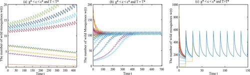
Example 4.1

Let the parameters a, μ, ξ, and $\overline{T}$ be given as $a=2,\mu =0.05,\xi =0.001,\overline{T}=14.$From (6(6) $s_h^{\ast }=\frac{a-\sqrt{a\mu }}{a}.$(6) ), (8(8) $g^{\ast }=\{\begin{array}{ll}{c}_0,& \mathrm{if}{s}_h\in (0,s_h^{\ast }],\\ c_1,& \mathrm{if}{s}_h\in (s_h^{\ast },1).\end{array}$(8) ), (9(9) $c^{\ast }=\frac{-a{s}_h+\sqrt{a^2{s}_h^2+4a{s}_h(1-s_h)(a-\mu )}}{2a\xi (1-s_h)},$(9) ) and (10(10) $T^{\ast }=\frac{a((\xi c-1)(1-s_h)+1)}{a-\mu }\cdot \overline{T}.$(10) ), we have $s_h^{\ast }=0.8419,g^{\ast }=787.5247,c^{\ast }=887.4855\mathrm{and}{T}^{\ast }=\mathrm{14.0574.}$We choose $s_h=0.9>s_h^{\ast }$ and $g^{\ast }<c=790<c^{\ast }$. The release period is set at $\overline{T}<T=14.04<T^{\ast }$. As shown in Figure 2(a), when the initial amount is small, the wild mosquitoes can be suppressed finally, implying that the origin $E_0$ is locally asymptotically stable, as stated by Theorem 3.1(1). If the release period T is set at $T=T^{\ast }$ or $T=15>T^{\ast }$, the amount of wild mosquitoes oscillates periodically around some level, as shown in Figures 2(b) and 2(c), which verifies the result given in Theorem 3.1(2). And we can find the amplitude increases with the release period.

Figure 2. The dynamical behaviours of Model (1(1) $\frac{\mathrm{d}w(t)}{\mathrm{d}t}=a(1-s_h\frac{g(t)}{w(t)+g(t)})(1-\xi (w(t)+g(t)))w(t)-\mu w(t),$(1) ) with $g^{\ast }<c<c^{\ast }$. (a) The origin $E_0$ is locally asymptotically stable with $T<T^{\ast }$. (b) Model (1(1) $\frac{\mathrm{d}w(t)}{\mathrm{d}t}=a(1-s_h\frac{g(t)}{w(t)+g(t)})(1-\xi (w(t)+g(t)))w(t)-\mu w(t),$(1) ) has a unique globally asymptotically stable T-periodic solution with $T=T^{\ast }$. (c) Model (1(1) $\frac{\mathrm{d}w(t)}{\mathrm{d}t}=a(1-s_h\frac{g(t)}{w(t)+g(t)})(1-\xi (w(t)+g(t)))w(t)-\mu w(t),$(1) ) has a unique globally asymptotically stable T-periodic solution with $T>T^{\ast }$.

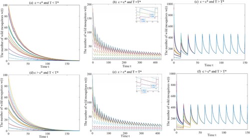
Example 4.2

Same as the above example, we select the same parameter values a, μ, ξ and $\overline{T}$, and get four thresholds $s_h^{\ast }$, $g^{\ast }$, $c^{\ast }$, and $T^{\ast }$. Choosing $s_h=0.9>s_h^{\ast }$ and $c=c^{\ast }$, if the release period $\overline{T}<T=14.01<T^{\ast }$ or $\overline{T}<T=T^{\ast }$, then the origin $E_0$ is globally asymptotically stable as shown in Figures 3(a) and 3(b). If $T=15>T^{\ast }$, then the amount of wild mosquitoes oscillates periodically as shown in Figure 3(c). Next, we choose $c=900>c^{\ast }$ and select $\overline{T}<T=14.01<T^{\ast }$, $\overline{T}<T=T^{\ast }$ or $T=15>T^{\ast }$, respectively. The same conclusions are reached (see Figure 3(d,e,f)).

Figure 3. The dynamical behaviours of Model (1(1) $\frac{\mathrm{d}w(t)}{\mathrm{d}t}=a(1-s_h\frac{g(t)}{w(t)+g(t)})(1-\xi (w(t)+g(t)))w(t)-\mu w(t),$(1) ) with $c\ge c^{\ast }$. (a) The origin $E_0$ is globally asymptotically stable with $c=c^{\ast }$ and $T<T^{\ast }$. (b) Model (1(1) $\frac{\mathrm{d}w(t)}{\mathrm{d}t}=a(1-s_h\frac{g(t)}{w(t)+g(t)})(1-\xi (w(t)+g(t)))w(t)-\mu w(t),$(1) ) has a unique globally asymptotically stable T-periodic solution with $c=c^{\ast }$ and $T=T^{\ast }$. (c) Model (1(1) $\frac{\mathrm{d}w(t)}{\mathrm{d}t}=a(1-s_h\frac{g(t)}{w(t)+g(t)})(1-\xi (w(t)+g(t)))w(t)-\mu w(t),$(1) ) has a unique globally asymptotically stable T-periodic solution with $c=c^{\ast }$ and $T>T^{\ast }$. (d) The origin $E_0$ is globally asymptotically stable with $c>c^{\ast }$ and $T<T^{\ast }$. (e) Model (1(1) $\frac{\mathrm{d}w(t)}{\mathrm{d}t}=a(1-s_h\frac{g(t)}{w(t)+g(t)})(1-\xi (w(t)+g(t)))w(t)-\mu w(t),$(1) ) has a unique globally asymptotically stable T-periodic solution with $c>c^{\ast }$ and $T=T^{\ast }$. (f) Model (1(1) $\frac{\mathrm{d}w(t)}{\mathrm{d}t}=a(1-s_h\frac{g(t)}{w(t)+g(t)})(1-\xi (w(t)+g(t)))w(t)-\mu w(t),$(1) ) has a unique globally asymptotically stable T-periodic solution with $c>c^{\ast }$ and $T>T^{\ast }$.

5. Conclusion

Based on the modelling methods of Yu [41] and Li [24], and the incomplete CI mechanism, we considered a population suppression model consisting of two sub-equations switching each other in this study by releasing Wolbachia-infected male mosquitoes. In modelling, we introduced the CI intensity $s_h\in (0,1)$ and the sexual lifespan $\overline{T}$ of Wolbachia-infected mosquitoes, and ignored the independent dynamical equation for Wolbachia-infected mosquitoes.

We assumed that the release amount $g(t)$ of Wolbachia-infected mosquitoes was periodic and impulsive at discrete time points $T_k=kT$, $k=0,1,2,\dots$, and focused on the case that the waiting period T was greater than the sexual lifespan $\overline{T}$. In this paper, we defined four thresholds: the CI intensity threshold $s_h^{\ast }$, the release amount thresholds $g^{\ast }$ and $c^{\ast }$, and the release waiting period threshold $T^{\ast }$. We obtained a relatively complete analysis for the dynamics of Model (1(1) $\frac{\mathrm{d}w(t)}{\mathrm{d}t}=a(1-s_h\frac{g(t)}{w(t)+g(t)})(1-\xi (w(t)+g(t)))w(t)-\mu w(t),$(1) ) when CI intensity $s_h$ is greater than its threshold $s_h^{\ast }$.

Several important lemmas were established and used to prove the main results. For many dynamical systems, it is challenging to obtain the conditions for the existence and uniqueness of periodic solutions. We established necessary and sufficient conditions for both the stability of the origin $E_0$ and the existence and uniqueness of the globally asymptotically stable T-periodic solution in Theorems 3.1 and 3.2, respectively.

In Theorem 3.1, we showed that when the conditions $s_h>s_h^{\ast }$ and $g^{\ast }<c<c^{\ast }$ hold, Model (1(1) $\frac{\mathrm{d}w(t)}{\mathrm{d}t}=a(1-s_h\frac{g(t)}{w(t)+g(t)})(1-\xi (w(t)+g(t)))w(t)-\mu w(t),$(1) ) has either a locally asymptotically stable origin $E_0$ or a unique globally asymptotically stable T-periodic solution depending on $T<T^{\ast }$ or $T\ge T^{\ast }$. That is, if we don't release enough Wolbachia-infected mosquitoes making the release amount be less than the threshold $c^{\ast }$, then whether the mosquito population is successfully suppressed depends on its initial value even though we release at a sufficient frequency $T<T^{\ast }$ (see Figure 2(a)). At the same time, when the mosquitoes are released infrequently, namely, $T\ge T^{\ast }$, then the suppression of mosquito population is unsuccessful (see Figure 2(b,c)). In Theorem 3.2, we obtained that when the conditions $s_h>s_h^{\ast }$ and $c\ge c^{\ast }$ hold, the globally asymptotically stable origin $E_0$ or the unique globally asymptotically stable T-periodic solution of Model (1(1) $\frac{\mathrm{d}w(t)}{\mathrm{d}t}=a(1-s_h\frac{g(t)}{w(t)+g(t)})(1-\xi (w(t)+g(t)))w(t)-\mu w(t),$(1) ) are obtained if $T\le T^{\ast }$ or $T>T^{\ast }$. In other words, if we release enough Wolbachia-infected mosquitoes ($c\ge c^{\ast }$) and release them frequently ($T\le T^{\ast }$), then the mosquito population will be suppressed (see Figure 3(a,b,e,d)). On the contrary, if the frequency of release is not frequent ($T>T^{\ast }$), then the mosquito population is persistent (see Figure 3(c,f)). Combining Theorems 3.1 and 3.2, under the conditions $s_h>s_h^{\ast }$ and $c>g^{\ast }$, the necessary and sufficient condition for the existence of the unique globally asymptotically stable T-periodic solution is that the origin $E_0$ is unstable.

In summary, we studied the dynamical behaviours of the wild mosquito population when $s_h>s_h^{\ast }$ and $c>g^{\ast }$, and gave complete conclusions and detailed steps. These studies have reference values for guiding mosquito control. The cases of $s_h\le s_h^{\ast }$ or $c\le g^{\ast }$ have not been studied, and these investigations are left to future work.

Disclosure statement

No potential conflict of interest was reported by the author(s).

Additional information

Funding

This work was supported by the National Natural Science Foundation of China [grant number 12171113].

References

- F. Baldacchino, B. Caputo, F. Chandre, A. Drago, A. della Torre, F. Montarsi, and A. Rizzoli, Control methods against invasive Aedes mosquitoes in Europe: A review, Pest Manag. Sci. 71 (2015), pp. 1471–1485.
- S. Boyer, J. Gilles, D. Merancienne, G. Lempérière, and D. Fontenille, Sexual performance of male mosquito Aedes albopictus, Med. Vet. Entomol. 25 (2011), pp. 454–459.
- O.J. Brady, P.W. Gething, S. Bhatt, J.P. Messina, J.S. Brownstein, A.G. Hoen, C.L. Moyes, A.W.Farlow, T.W. Scott, S.I. Hay, and R. Reithinger, Refining the global spatial limits of dengue virus transmission by evidence-based consensus, Plos Neglect. Trop. D 6(8) (2012), pp. 1–15.
- J.S. Brownstein, E. Hett, and S.L. O'Neill, The potential of virulent Wolbachia to modulate disease transmission by insects, J. Invertebr. Pathol. 84 (2003), pp. 24–29.
- L.M. Cai, S. Ai, and J. Li, Dynamics of mosquitoes populations with different strategies for releasing sterile mosquitoes, SIAM J. Appl. Math. 74(6) (2014), pp. 1786–1809.
- L.M. Cai, S. Ai, and G. Fan, Dynamics of delayed mosquitoes populations models with two different strategies of releasing sterile mosquitoes, Math. Biosci. Eng. 15(5) (2018), pp. 1181–1202.
- L.M. Cai, J. Huang, X.Y. Song, and Y.Y. Zhang, Bifurcation analysis of a mosquito population model for proportional releasing sterile mosquitoes, Discrete Contin. Dyn. Syst. B 24(11) (2019), pp. 6279–6295.
- E. Caspari and G.S. Watson, On the evolutionary importance of cytoplasmic sterility in mosquitoes, Evolution 13(4) (1959), pp. 568–570.
- J. Cohen, Dengue may bring out the worst in Zika, Science 355(6332) (2017), p. 1362.
- J.E. Crawford, D.W. Clarke, V. Criswell, M. Desnoyer, D. Cornel, B. Deegan, K. Gong, K.C. Hopkins, P. Howell, J.S. Hyde, J. Livni, C. Behling, R. Benza, W. Chen, K.L. Dobson, C. Eldershaw, D. Greeley, Y. Han, B. Hughes, E. Kakani, J. Karbowski, A. Kitchell, E. Lee, T. Lin, J. Liu, M. Lozano, W.MacDonald, J.W. Mains, M. Metlitz, S.N. Mitchell, D. Moore, J.R. Ohm, K. Parkes, A. Porshnikoff, C. Robuck, M. Sheridan, R. Sobecki, P. Smith, J. Stevenson, J. Sullivan, B. Wasson, A.M. Weakley, M. Wilhelm, J. Won, A. Yasunaga, W.C. Chan, J. Holeman, N. Snoad, L. Upson, T. Zha, S.L. Dobson, F.S. Mulligan, P. Massaro, and B.J. White, Efficient production of male Wolbachia-infected Aedes aegypti mosquitoes enables large-scale suppression of wild populations, Nat. Biotechnol. 38 (2020), pp. 482–492.
- W. Dejnirattisai, P. Supasa, W. Wongwiwat, A. Rouvinski, G. Barba-Spaeth, T. Duangchinda, A.Sakuntabhai, V.-M. Cao-Lormeau, P. Malasit, F.A. Rey, J. Mongkolsapaya, and G.R. Screaton, Dengue virus sero-cross-reactivity drives antibody-dependent enhancement of infection with Zika virus, Nat. Immunol. 17(9) (2016), pp. 1102–1108.
- C. Dye, Intraspecific competition amongst larval Aedes aegypti: Food exploitation or chemical interference, Ecol. Entomol. 7(1) (1982), pp. 39–46.
- J.Z. Farkas and P. Hinow, Structured and unstructured continuous models for Wolbachia infections, Bull. Math. Biol. 72 (2010), pp. 2067–2088.
- R.M. Gleiser, J. Urrutia, and D.E. Gorla, Effects of crowding on populations of Aedes albifasciatus larvae under laboratory conditions, Entomol. Exp. Appl. 95(2) (2000), pp. 135–140.
- A.A. Hoffmann, B.L. Montgomery, J. Popovici, I. Iturbe-Ormaetxe, P.H. Johnson, F. Muzzi, M.Greenfield, M. Durkan, Y.S. Leong, Y. Dong, H. Cook, J. Axford, A.G. Callahan, N. Kenny, C.Omodei, E.A. McGraw, P.A. Ryan, S.A. Ritchie, M. Turelli, and S.L. O'Neill, Successful establishment of Wolbachia in Aedes populations to suppress dengue transmission, Nature 476 (2011), pp. 454–457.
- L. Hu, M. Huang, M. Tang, J. Yu, and B. Zheng, Wolbachia spread dynamics in stochastic environments, Theor. Popul. Biol. 106 (2015), pp. 32–44.
- L. Hu, M. Tang, Z. Wu, Z. Xi, and J. Yu, The threshold infection level for Wolbachia invasion in random environments, J. Differ. Equ. 266 (2019), pp. 4377–4393.
- M.G. Huang, M.X. Tang, and J.S. Yu, Wolbachia infection dynamics by reaction-diffusion equations, Sci. China Math. 58(1) (2015), pp. 77–96.
- A. Jeyaprakash and M.A. Hoy, Long PCR improves Wolbachia DNA amplification: Wsp sequences found in 76% of sixty-three arthropod species, Insect Mol. Biol. 9 (2000), pp. 393–405.
- M.J. Keeling, F.M. Jiggins, and J.M. Read, The invasion and coexistence of competing Wolbachia strains, Heredity 91 (2003), pp. 382–388.
- H. Laven, Cytoplasmic inheritance in Culex, Nature 177 (1956), pp. 141–142.
- J. Li, Simple mathematical models for interacting wild and transgenic mosquito populations, Math. Biosci. 189 (2004), pp. 39–59.
- J. Li, Differential equations models for interacting wild and transgenic mosquito populations, J. Biol. Dyn. 2(3) (2008), pp. 241–258.
- J. Li, New revised simple models for interactive wild and sterile mosquito populations and their dynamics, J. Biol. Dyn. 11(S2) (2017), pp. 316–333.
- Y. Li, F. Kamara, G. Zhou, S. Puthiyakunnon, C. Li, Y. Liu, Y. Zhou, L. Yao, G. Yan, X.-G. Chen, and P. Kittayapong, Urbanization increases Aedes albopictus larval habitats and accelerates mosquito development and survivorship, PLoS Negl. Trop. Dis. 8 (2014), p. e3301.
- G.H. Lin and Y.X. Hui, Stability analysis in a mosquito population suppression model, J. Biol. Dyn. 14(1) (2020), pp. 578–589.
- F.S. Liu, C.S. Yao, P.Q. Lin, and C.Q. Zhou, Studies on life table of the natural population of Aedes albopictus, Acta Sci. Nat. Univ. Sunyatseni 31(8) (1992), pp. 84–93.
- Y.F. Liu, F. Jiao, and L.C. Hu, Modeling mosquito population control by a coupled system, J. Math. Anal. Appl. 506 (2022), p. 125671.
- C.J. McMeniman, R.V. Lane, B.N. Cass, A.W.C. Fong, M. Sidhu, Y.-F. Wang, and S. L. O'Neill, Stable introduction of a life-shortening Wolbachia infection into the mosquito Aedes aegypti, Science 323 (2009), pp. 141–144.
- J.L. Rasgon and T.W. Scott, Impact of population age structure on Wolbachia transgene driver efficacy: Ecologically complex factors and release of genetically modified mosquitoes, Insect Biochem. Mol. Biol. 34 (2004), pp. 707–713.
- P. Schofield, Spatially explicit models of Turelli-Hoffmann Wolbachia invasive wave fronts, J. Theor. Biol. 215 (2002), pp. 121–131.
- P. Somwang, J. Yanola, W. Suwan, C. Walton, N. Lumjuan, L. Prapanthadara, and P. Somboon, Enzymes-based resistant mechanism in pyrethroid resistant and susceptible Aedes aegypti strains from northern Thailand, Parasitol. Res. 109 (2011), pp. 531–537.
- M. Turelli, Evolution of incompatibility-inducing microbes and their hosts, Evolution 48(5) (1994), pp. 1500–1513.
- Y. Wang, X. Liu, C.L. Li, S. Tianyun, J. Jin, Y. Guo, D. Ren, Z. Yang, Q. Liu, and F. Meng, A survey of insecticide resistance in Aedes albopictus (Diptera: Culicidae) during a 2014 dengue fever outbreak in Guangzhou China, J. Econ. Entomol. 110(1) (2017), pp. 239–244.
- J.H. Werren, D. Windsor, and L. Gao, Distribution of Wolbachia among neotropical arthropods, Proc. R. Soc. Lond. B 262 (1995), pp. 197–204.
- WHO, Dengue: Guidelines for Diagnosis, Treatment, Prevention and Control, World Health Organization, Geneva, 2009.
- WHO, Vector-borne diseases, 2 March 2020. Available at https://www.who.int/news-room/fact-sheets/detail/vector-borne-diseases.
- WHO, Dengue and severe dengue, 19 May 2021. Available at https://www.who.int/news-room/fact-sheets/detail/dengue-and-severe-dengue.
- Z.Y. Xi, C.C.H. Khoo, and S.L. Dobson, Wolbachia establishment and invasion in an Aedes aegypti laboratory population, Science 310 (2005), pp. 326–328.
- Z.Y. Xi, C.C.H. Khoo, and S.L. Dobson, Interspecific transfer of Wolbachia into the mosquito disease vector Aedes albopictus, Proc. R. Soc. B 273 (2006), pp. 1317–1322.
- J.S. Yu, Modelling mosquito population suppression based on delay differential equations, SIAM J. Appl. Math. 78(6) (2018), pp. 3168–3187.
- J.S. Yu, Existence and stability of a unique and exact two periodic orbits for an interactive wild and sterile mosquito model, J. Differ. Equ. 269 (2020), pp. 10395–10415.
- J.S. Yu and J. Li, Dynamics of interactive wild and sterile mosquitoes with time delay, J. Biol. Dyn. 13(1) (2019), pp. 606–620.
- J.S. Yu and J. Li, Global asymptotic stability in an interactive wild and sterile mosquito model, J. Differ. Equ. 269 (2020), pp. 6193–6215.
- J.S. Yu and B. Zheng, Modelling Wolbachia infection in mosquito population via discrete dynamical models, J. Differ. Equ. Appl. 25(11) (2019), pp. 1549–1567.
- D. Zhang, X. Zheng, Z. Xi, K. Bourtzis, J.R.L. Gilles, and R. Cordaux, Combining the sterile insect technique with the incompatible insect technique: I-Impact of Wolbachia infection on the fitness of triple-and double-infected strains of Aedes albopictus, PLoS One 10 (2015), p. e0121126.
- B. Zheng and J.S. Yu, Existence and uniqueness of periodic orbits in a discrete model on Wolbachia infection frequency, Adv. Nonlinear Anal. 11 (2022), pp. 212–224.
- X. Zheng, D. Zhang, Y. Li, C. Yang, Y. Wu, X. Liang, Y. Liang, X. Pan, L. Hu, Q. Sun, X. Wang, Y.Wei, J. Zhu, W. Qian, Z. Yan, A.G. Parker, J.R.L. Gilles, K. Bourtzis, J. Bouyer, M. Tang, B. Zheng, J. Yu, J. Liu, J. Zhuang, Z. Hu, M. Zhang, J.-T. Gong, X.-Y. Hong, Z. Zhang, L. Lin, Q. Liu, Z. Hu, Z. Wu, L.A. Baton, A.A. Hoffmann, and Z. Xi, Incompatible and sterile insect techniques combined eliminate mosquitoes, Nature 572 (2019), pp. 56–61.
- B. Zheng, J.S. Yu, and J. Li, Modeling and analysis of the implementation of the Wolbachia incompatible and sterile insect technique for mosquito population suppression, SIAM J. Appl. Math. 81(2) (2021), pp. 718–740.
- B. Zheng, J. Li, and J.S. Yu, One discrete dynamical model on Wolbachia infection frequency in mosquito populations, Sci. China Math. (2022). https://doi.org/10.1007/s11425-021-1891-7.