Impact of information and Lévy noise on stochastic COVID-19 epidemic model under real statistical data

Abstract

In this paper, we consider the dynamical behaviour of a stochastic coronavirus (COVID-19) susceptible-infected-removed epidemic model with the inclusion of the influence of information intervention and Lévy noise. The existence and uniqueness of the model positive solution are proved. Then, we establish a stochastic threshold as a sufficient condition for the extinction and persistence in mean of the disease. Based on the available COVID-19 data, the parameters of the model were estimated and we fit the model with real statistics. Finally, numerical simulations are presented to support our theoretical results.

Keywords:

• Stochastic COVID-19 model
• Lévy jump
• information intervention
• extinction
• persistence
• numerical simulation

1. Introduction

As we all know, the epidemic infectious diseases cause a profound impact on the safety of human life and property. In order to better control infectious diseases, scholars in various research directions have made positive contributions to improve the health policy. For example, the $H7N9$ bird flu, all patients infected with the virus had fever in the early stage, was first reported in Shanghai and Anhui at the end of March 2013. After the outbreak of infectious diseases, how to develop effective treatment measures has become a hot research issue. With the strengthening of media reports and health education, people's awareness of epidemic prevention has gradually improved, which can prevent or delay the occurrence of diseases to a certain extent. This non-drug therapy combined with the drug treatment has yield twice the result with half the effort, especially in the treatment of COVID-19 [6, 14, 19, 20].

In addition, combined the knowledge of a stochastic and differential dynamic system, mathematical model becomes one of the most important measure in controlling the pandemic of the disease (see, e.g. Refs. [2, 17, 19]). It is far enough to understand the dynamics of disease transmission; with using the mathematical model and the knowledge of optimal control, remarkable achievements have been made in disease control [8, 21, 22]. The main feature of the infectious disease model is to analyze the disease transmission dynamics from the theoretical part. Otherwise, knowledge in the field of optimal control plays a fundamental role in controlling the transmission of disease effectively. Two main types of models are widely used in modelling the dynamics of disease: deterministic and stochastic. For the deterministic model, considering the local and global stability of the mathematical part and using the optimal control strategies for the epidemic models coupled with nonlinear incidence functions are common theoretical analysis methods which are deeply studied by some researchers [18, 22]. On the other hand, for the stochastic model, the stability analysis receives attention and is widely used in modelling the real dynamics of the disease [9, 16, 18]. While comparing the deterministic model, the stochastic model is more fit in the real date of the epidemic disease.

It is widely known that the Gauss noise is commonly used in modelling the stochastic properties of the infectious disease. While comparing with the Gauss white noise, the Levy noise is superior to the Gauss noise in the epidemic model as shown in Refs. [5, 12, 13], despite its mathematical complexity. For some epidemic diseases, which significantly affect the environment noise and the scaled drift velocity falls inside an interval that depends on the threshold values, the advantage of the Levy noise is clearly embodied. Proved by the global and local Lipschitz conditions in some general stochastic differential equation, the additive levy noise can increase the intensity of mutual information in several feedback epidemic models. Due to the Levy noise model, not just takes consideration of only pure-diffusion or pure-jump models but combine these two processes together, so it can accurately describe how the potential of neurons membrane evolves as compared to a simpler diffusion model. Therefore, the model taking the Levy noise into consideration has obvious advantages in modelling the time-varying recurrent neural networks.

In this article, based on stochastic theory, we set up an classical infectious disease model and then investigate the dynamics of COVID-19 epidemic in which we consider the influence of Levy noise. In consideration of the characteristic and the varying population environment, we showed the light on the dynamics of COVID-19 by utilizing the susceptible-infected-removed (SIR) epidemic model. (1) $\begin{array}{rl}\frac{\mathrm{d}S\left(t\right)}{\mathrm{d}t}& =\mathrm{\Pi }-\eta S\left(t\right)I\left(t\right)-(\delta +d)S\left(t\right),\\ \frac{\mathrm{d}I\left(t\right)}{\mathrm{d}t}& =\eta I\left(t\right)S\left(t\right)-(d+{\gamma }_1+{\mu }_1)I\left(t\right),\\ \frac{\mathrm{d}R\left(t\right)}{\mathrm{d}t}& ={\gamma }_{1}I\left(t\right)+\delta S\left(t\right)-\mathrm{d}R\left(t\right).\end{array}$(1) In order to meet the biological significance, all the parameters must be positive and have the following signification:

1. Π: Per capita new born susceptible individuals.

2. d: Natural death rate.

3. ${\mu }_1$: The death rate due to COVID-19.

4. η: The infected rate of susceptible.

5. δ: Vaccination rate of COVID-19.

6. ${\gamma }_1$: The rate of recovering.

To further consider the impact of environmental fluctuations on disease transmission [10, 11, 15], the commonly used methods by many researchers are introducing Gauss white noise in Equation (1(1) $\begin{array}{rl}\frac{\mathrm{d}S\left(t\right)}{\mathrm{d}t}& =\mathrm{\Pi }-\eta S\left(t\right)I\left(t\right)-(\delta +d)S\left(t\right),\\ \frac{\mathrm{d}I\left(t\right)}{\mathrm{d}t}& =\eta I\left(t\right)S\left(t\right)-(d+{\gamma }_1+{\mu }_1)I\left(t\right),\\ \frac{\mathrm{d}R\left(t\right)}{\mathrm{d}t}& ={\gamma }_{1}I\left(t\right)+\delta S\left(t\right)-\mathrm{d}R\left(t\right).\end{array}$(1) ). In order to simulate the fluctuation of the environment, one of the standard approaches is to adjust the parameters fluctuate around a mean value caused by continuous fluctuations in the environment [1, 4, 7]. Many researchers find that the basic reproduction number of the disease can be deeply influenced by the ambient white noise [10, 15, 16]. However, when we treat the environment fluctuation equivalently as Levy noise and combine the real data, what effect will give rise to the dynamics of COVID-19 still remains unknown.

Based on what we discuss above, we introduce an extending model in system (1(1) $\begin{array}{rl}\frac{\mathrm{d}S\left(t\right)}{\mathrm{d}t}& =\mathrm{\Pi }-\eta S\left(t\right)I\left(t\right)-(\delta +d)S\left(t\right),\\ \frac{\mathrm{d}I\left(t\right)}{\mathrm{d}t}& =\eta I\left(t\right)S\left(t\right)-(d+{\gamma }_1+{\mu }_1)I\left(t\right),\\ \frac{\mathrm{d}R\left(t\right)}{\mathrm{d}t}& ={\gamma }_{1}I\left(t\right)+\delta S\left(t\right)-\mathrm{d}R\left(t\right).\end{array}$(1) ) and draw on relevant methods from Ref. [3] information intervention and added Lévy. Due to the dual effect of environmental noise (Gauss noise) and Lévy noise, we assume that the noise intensities are proportional to each state $S\left(t\right),I\left(t\right),R\left(t\right)$ and $X\left(t\right)$. In this way, the deterministic model (1(1) $\begin{array}{rl}\frac{\mathrm{d}S\left(t\right)}{\mathrm{d}t}& =\mathrm{\Pi }-\eta S\left(t\right)I\left(t\right)-(\delta +d)S\left(t\right),\\ \frac{\mathrm{d}I\left(t\right)}{\mathrm{d}t}& =\eta I\left(t\right)S\left(t\right)-(d+{\gamma }_1+{\mu }_1)I\left(t\right),\\ \frac{\mathrm{d}R\left(t\right)}{\mathrm{d}t}& ={\gamma }_{1}I\left(t\right)+\delta S\left(t\right)-\mathrm{d}R\left(t\right).\end{array}$(1) ) can be extended into a stochastic one as listed below: (2) $\begin{array}{rl}\mathrm{d}S\left(t\right)& =[\mathrm{\Pi }-{\mu }_{2}mX(t\left)S\right(t)-\eta S(t\left)I\right(t)-(\delta +d\left)S\right(t\left)\right]\mathrm{d}t\\ & +{\xi }_{1}S\left(t\right)\mathrm{d}{W}_1\left(t\right)\\ & +{\int }_Y{B}_1\left(y\right)S\left(t^{-}\right)\tilde{N}(\mathrm{d}t,\mathrm{d}y),\\ \mathrm{d}I\left(t\right)& =\left[\eta I\right(t\left)S\right(t)-(d+{\gamma }_1+{\mu }_1\left)I\right(t\left)\right]\mathrm{d}t+{\xi }_{2}I\left(t\right)\mathrm{d}{W}_2\left(t\right)\\ & +{\int }_Y{B}_2\left(y\right)I\left(t^{-}\right)\tilde{N}(\mathrm{d}t,\mathrm{d}y),\\ \mathrm{d}R\left(t\right)& =\left[{\gamma }_{1}I\right(t)+{\mu }_{2}mX(t\left)S\right(t)+\delta S(t)-\mathrm{d}R(t\left)\right]\mathrm{d}t+{\xi }_{3}R\left(t\right)\mathrm{d}{W}_3\left(t\right)\\ & +{\int }_Y{B}_3\left(y\right)R\left(t^{-}\right)\tilde{N}(\mathrm{d}t,\mathrm{d}y),\\ \mathrm{d}X\left(t\right)& =[\frac{{\mu }_{3}I\left(t\right)}{(1+hI(t\left)\right)}-aX(t\left)\right]\mathrm{d}t+{\xi }_{4}X\left(t\right)\mathrm{d}{W}_4\left(t\right)+{\int }_Y{B}_4\left(y\right)X\left(t^{-}\right)\tilde{N}(\mathrm{d}t,\mathrm{d}y),\end{array}$(2) where the $W_1\left(t\right),W_2\left(2\right),W_3\left(t\right)$ and $W_4\left(t\right)$ represent the Brownian motions and ${\xi }_1,{\xi }_2,{\xi }_3$ and ${\xi }_4$ represent the noise intensity. Obviously, the Brownian motion will satisfy the basic axiom of $W_1\left(0\right)=W_2\left(0\right)=W_3\left(0\right)=W_4\left(0\right)=0.Z\left(t^{-}\right)$ stands for the left limit of $Z\left(t\right)$. $\tilde{N}$ denotes the compensated random measure defined by $\tilde{N}=N(\mathrm{d}t,\mathrm{d}y)-v\left(\mathrm{d}y\right)\mathrm{d}t$ and $N(\mathrm{d}t,\mathrm{d}y)$ is a Poisson counting measure with the stationary compensator $v\left(\mathrm{d}y\right)\mathrm{d}t$. v is defined on a measurable subset Q of $[0,+\mathrm{\infty })$ with $v\left(\mathrm{Q}\right)<\mathrm{\infty }$ and $B_i>-1,i=1,2,3,4.$ Here, $S\left(t\right),I\left(t\right)$ and $R\left(t\right)$ represent the susceptible, infected and recovered individuals in the area, $X\left(t\right)$ stands for the information density of the population, where m is the information interaction rate caused by individuals who change their behaviour, ${\mu }_3$ represents the rate of information growth, ${\mu }_2$ represents the response intensity, h is the saturation constant and a is the natural degradation of information.

The rest of the paper is organized as follows: in Section 2, we show that the model preserves the properties of existence and uniqueness. The sufficient condition of the extinction about the disease is shown in Section 3. As shown in Section 4, we proof the persistence of the disease. Subsequently, the model results have been verified with the help of numerical simulations and fitted by the real data in Section 5. The work has been finished in Section 6 with a brief conclusion.

2. Existence and uniqueness of positive solution

The existence as well as the unique global positive solution of the system's (2(2) $\begin{array}{rl}\mathrm{d}S\left(t\right)& =[\mathrm{\Pi }-{\mu }_{2}mX(t\left)S\right(t)-\eta S(t\left)I\right(t)-(\delta +d\left)S\right(t\left)\right]\mathrm{d}t\\ & +{\xi }_{1}S\left(t\right)\mathrm{d}{W}_1\left(t\right)\\ & +{\int }_Y{B}_1\left(y\right)S\left(t^{-}\right)\tilde{N}(\mathrm{d}t,\mathrm{d}y),\\ \mathrm{d}I\left(t\right)& =\left[\eta I\right(t\left)S\right(t)-(d+{\gamma }_1+{\mu }_1\left)I\right(t\left)\right]\mathrm{d}t+{\xi }_{2}I\left(t\right)\mathrm{d}{W}_2\left(t\right)\\ & +{\int }_Y{B}_2\left(y\right)I\left(t^{-}\right)\tilde{N}(\mathrm{d}t,\mathrm{d}y),\\ \mathrm{d}R\left(t\right)& =\left[{\gamma }_{1}I\right(t)+{\mu }_{2}mX(t\left)S\right(t)+\delta S(t)-\mathrm{d}R(t\left)\right]\mathrm{d}t+{\xi }_{3}R\left(t\right)\mathrm{d}{W}_3\left(t\right)\\ & +{\int }_Y{B}_3\left(y\right)R\left(t^{-}\right)\tilde{N}(\mathrm{d}t,\mathrm{d}y),\\ \mathrm{d}X\left(t\right)& =[\frac{{\mu }_{3}I\left(t\right)}{(1+hI(t\left)\right)}-aX(t\left)\right]\mathrm{d}t+{\xi }_{4}X\left(t\right)\mathrm{d}{W}_4\left(t\right)+{\int }_Y{B}_4\left(y\right)X\left(t^{-}\right)\tilde{N}(\mathrm{d}t,\mathrm{d}y),\end{array}$(2) ) with relapse and jumps are discussed in this section, utilizing the similar reasoning as in Ref. [13]. We will use two classical hypotheses, $\left({\mathbf{H}}_{\mathbf{1}}\right)$ and $\left({\mathbf{H}}_{\mathbf{2}}\right)$, to justify the existence and uniqueness of a global positive solution of (2(2) $\begin{array}{rl}\mathrm{d}S\left(t\right)& =[\mathrm{\Pi }-{\mu }_{2}mX(t\left)S\right(t)-\eta S(t\left)I\right(t)-(\delta +d\left)S\right(t\left)\right]\mathrm{d}t\\ & +{\xi }_{1}S\left(t\right)\mathrm{d}{W}_1\left(t\right)\\ & +{\int }_Y{B}_1\left(y\right)S\left(t^{-}\right)\tilde{N}(\mathrm{d}t,\mathrm{d}y),\\ \mathrm{d}I\left(t\right)& =\left[\eta I\right(t\left)S\right(t)-(d+{\gamma }_1+{\mu }_1\left)I\right(t\left)\right]\mathrm{d}t+{\xi }_{2}I\left(t\right)\mathrm{d}{W}_2\left(t\right)\\ & +{\int }_Y{B}_2\left(y\right)I\left(t^{-}\right)\tilde{N}(\mathrm{d}t,\mathrm{d}y),\\ \mathrm{d}R\left(t\right)& =\left[{\gamma }_{1}I\right(t)+{\mu }_{2}mX(t\left)S\right(t)+\delta S(t)-\mathrm{d}R(t\left)\right]\mathrm{d}t+{\xi }_{3}R\left(t\right)\mathrm{d}{W}_3\left(t\right)\\ & +{\int }_Y{B}_3\left(y\right)R\left(t^{-}\right)\tilde{N}(\mathrm{d}t,\mathrm{d}y),\\ \mathrm{d}X\left(t\right)& =[\frac{{\mu }_{3}I\left(t\right)}{(1+hI(t\left)\right)}-aX(t\left)\right]\mathrm{d}t+{\xi }_{4}X\left(t\right)\mathrm{d}{W}_4\left(t\right)+{\int }_Y{B}_4\left(y\right)X\left(t^{-}\right)\tilde{N}(\mathrm{d}t,\mathrm{d}y),\end{array}$(2) ).

(H1).

For every $\mathbb{M}>0$ ∃${\mathbb{L}}_{\mathbb{M}}>0$∋ ${\int }_{\mathrm{{\rm Y}}}{|Q_{\iota }({\chi }_1,\mathrm{{\rm Y}})-Q_{\iota }({\chi }_2,\mathrm{{\rm Y}})|}^{2}v\left(\mathrm{d}\mathrm{{\rm Y}}\right)\le {\mathbb{L}}_{\mathbb{M}}{|{\chi }_1-{\chi }_2|}^2,\iota =1,2,3,4,$for $|{\mathrm{{\rm Y}}}_1|\vee |{\mathrm{{\rm Y}}}_2|\le \mathbb{M}$ wherein $\begin{array}{rl}{Q}_1(\chi ,\mathrm{{\rm Y}})& =B_1\left(\mathrm{{\rm Y}}\right)\chi \mathrm{f}\mathrm{o}\mathrm{r}\chi =\mathcal{S}\left(t^{-}\right),\\ Q_2(\chi ,\mathrm{{\rm Y}})& =B_2\left(\mathrm{{\rm Y}}\right)\chi \mathrm{f}\mathrm{o}\mathrm{r}\chi =\mathcal{I}\left(t^{-}\right),\\ Q_3(\chi ,\mathrm{{\rm Y}})& =B_3\left(\mathrm{{\rm Y}}\right)\chi \mathrm{f}\mathrm{o}\mathrm{r}\chi =\mathcal{R}\left(t^{-}\right),\\ Q_4(\chi ,\mathrm{{\rm Y}})& =B_4\left(\mathrm{{\rm Y}}\right)\chi \mathrm{f}\mathrm{o}\mathrm{r}\chi =X\left(t^{-}\right).\end{array}$

(H2).

$|\log \left(B_{\iota }\right(\chi \left)\right)|\le C$ for $B_{\iota }\left(\chi \right)>-1,\iota =1,2,3,4$, with C being a positive constant.

Theorem 2.1

For every specified initial value $\left(\mathcal{S}\right(0),\mathcal{I}(0),\mathcal{R}(0),X(0\left)\right)\in {\mathbb{R}}_{+}^4$, model (2(2) $\begin{array}{rl}\mathrm{d}S\left(t\right)& =[\mathrm{\Pi }-{\mu }_{2}mX(t\left)S\right(t)-\eta S(t\left)I\right(t)-(\delta +d\left)S\right(t\left)\right]\mathrm{d}t\\ & +{\xi }_{1}S\left(t\right)\mathrm{d}{W}_1\left(t\right)\\ & +{\int }_Y{B}_1\left(y\right)S\left(t^{-}\right)\tilde{N}(\mathrm{d}t,\mathrm{d}y),\\ \mathrm{d}I\left(t\right)& =\left[\eta I\right(t\left)S\right(t)-(d+{\gamma }_1+{\mu }_1\left)I\right(t\left)\right]\mathrm{d}t+{\xi }_{2}I\left(t\right)\mathrm{d}{W}_2\left(t\right)\\ & +{\int }_Y{B}_2\left(y\right)I\left(t^{-}\right)\tilde{N}(\mathrm{d}t,\mathrm{d}y),\\ \mathrm{d}R\left(t\right)& =\left[{\gamma }_{1}I\right(t)+{\mu }_{2}mX(t\left)S\right(t)+\delta S(t)-\mathrm{d}R(t\left)\right]\mathrm{d}t+{\xi }_{3}R\left(t\right)\mathrm{d}{W}_3\left(t\right)\\ & +{\int }_Y{B}_3\left(y\right)R\left(t^{-}\right)\tilde{N}(\mathrm{d}t,\mathrm{d}y),\\ \mathrm{d}X\left(t\right)& =[\frac{{\mu }_{3}I\left(t\right)}{(1+hI(t\left)\right)}-aX(t\left)\right]\mathrm{d}t+{\xi }_{4}X\left(t\right)\mathrm{d}{W}_4\left(t\right)+{\int }_Y{B}_4\left(y\right)X\left(t^{-}\right)\tilde{N}(\mathrm{d}t,\mathrm{d}y),\end{array}$(2) ) has a distinct global solution $\left(\mathcal{S}\right(t),\mathcal{I}(t),\mathcal{R}(t),X(t\left)\right)\in {\mathbb{R}}_{+}^4$ ∀ $t\ge 0$ a.s.

Proof.

Because the drift as well as diffusion are locally Lipschitz, there will be a unique local solution $\left(\mathcal{S}\right(t),\mathcal{I}(t),\mathcal{R}(t),X(t\left)\right)$ over $t\in [0,{\zeta }_e)$ about any known initial state $\left(\mathcal{S}\right(0),\mathcal{I}(0),\mathcal{R}(0),X(0\left)\right)\in {\mathbb{R}}_{+}^4$, where ${\zeta }_e$ is the blow time. We need to show that $\tau =\mathrm{\infty }$ a.s. to establish that this solution is global. To begin, we show that $\left(\mathcal{S}\right(t),\mathcal{I}(t),\mathcal{R}(t),X(t\left)\right)$ does not blow to infinity in a finite period of time. Allow $k_0>0$ to be large enough such that $\left(\mathcal{S}\right(0),\mathcal{I}(0),\mathcal{R}(0),X(0\left)\right)$ falls within the range $[1/k_0,k_0]$. Let us specify the stopping time for every number $k\le k_0$. (3) ${\zeta }_k=inf\{t\in [0,{\zeta }_e)/(\mathcal{S}\left(t\right),\mathcal{I}\left(t\right),\mathcal{R}\left(t\right),X\left(t\right))\notin (\frac{1}{k},k)\}.$(3) One may readily observe that ${\zeta }^{+}\le {\zeta }_e$ when we set $infset=\mathrm{\infty }$, therefore demonstrating that ${\zeta }^{+}=\mathrm{\infty }$ a.s. demonstrates that ${\zeta }_e=+\mathrm{\infty }$ a.s. If we presume that ${\zeta }^{+}<\mathrm{\infty }$, then there still exists $\mathcal{T}>0$ so that $\mathbb{P}({\zeta }^{+}<\mathcal{T})>0$.

Bearing in mind the following function, we will also use an operator $H:{\mathbb{R}}_{+}^4\to {\mathbb{R}}_{+}$ from the $C^2$ space as follows: (4) $\begin{array}{rl}& H(\mathcal{S},\mathcal{I},\mathcal{R},X)\\ & =(\mathcal{S}-C-C\frac{\mathrm{l}\mathrm{o}\mathrm{g}\mathcal{S}}{C})+(\mathcal{I}-1-\mathrm{l}\mathrm{o}\mathrm{g}\mathcal{I})+(\mathcal{R}-1-\mathrm{l}\mathrm{o}\mathrm{g}\mathcal{R})+(X-1-\mathrm{l}\mathrm{o}\mathrm{g}X).\end{array}$(4) Applying $It\hat{o}$ formula to H for all $t\in [0,{\zeta }^{+}]$, and C will be determined later. (5) $\begin{array}{rl}\mathrm{d}H& =LH(\mathcal{S},\mathcal{I},\mathcal{R},X)\mathrm{d}t+{\xi }_1(\mathcal{S}-C)\mathrm{d}{W}_1\left(t\right)+{\xi }_2(\mathcal{I}-1)\mathrm{d}{W}_2\left(t\right)\\ & +{\xi }_3(\mathcal{R}-1)\mathrm{d}{W}_3\left(t\right)+{\xi }_4(X-1)\mathrm{d}{W}_4\left(t\right)\\ & +{\int }_{\mathrm{{\rm Y}}}\left[B_1\right(\mathrm{{\rm Y}})\mathcal{S}-C\log (1+B_1(\mathrm{{\rm Y}}\left)\right)]\tilde{N}(\mathrm{d}t,\mathrm{d}\mathrm{{\rm Y}})\\ & +{\int }_{\mathrm{{\rm Y}}}\left[B_2\right(\mathrm{{\rm Y}})\mathcal{I}-\log (1+B_2(\mathrm{{\rm Y}}\left)\right)]\tilde{N}(\mathrm{d}t,\mathrm{d}\mathrm{{\rm Y}})\\ & +{\int }_{\mathrm{{\rm Y}}}\left[B_3\right(\mathrm{{\rm Y}})\mathcal{R}-\log (1+B_3(\mathrm{{\rm Y}}\left)\right)]\tilde{N}(\mathrm{d}t,\mathrm{d}\mathrm{{\rm Y}})\\ & +{\int }_{\mathrm{{\rm Y}}}\left[B_4\right(\mathrm{{\rm Y}})X-\log (1+B_4(\mathrm{{\rm Y}}\left)\right)]\tilde{N}(\mathrm{d}t,\mathrm{d}\mathrm{{\rm Y}}).\end{array}$(5) In Equation (5(5) $\begin{array}{rl}\mathrm{d}H& =LH(\mathcal{S},\mathcal{I},\mathcal{R},X)\mathrm{d}t+{\xi }_1(\mathcal{S}-C)\mathrm{d}{W}_1\left(t\right)+{\xi }_2(\mathcal{I}-1)\mathrm{d}{W}_2\left(t\right)\\ & +{\xi }_3(\mathcal{R}-1)\mathrm{d}{W}_3\left(t\right)+{\xi }_4(X-1)\mathrm{d}{W}_4\left(t\right)\\ & +{\int }_{\mathrm{{\rm Y}}}\left[B_1\right(\mathrm{{\rm Y}})\mathcal{S}-C\log (1+B_1(\mathrm{{\rm Y}}\left)\right)]\tilde{N}(\mathrm{d}t,\mathrm{d}\mathrm{{\rm Y}})\\ & +{\int }_{\mathrm{{\rm Y}}}\left[B_2\right(\mathrm{{\rm Y}})\mathcal{I}-\log (1+B_2(\mathrm{{\rm Y}}\left)\right)]\tilde{N}(\mathrm{d}t,\mathrm{d}\mathrm{{\rm Y}})\\ & +{\int }_{\mathrm{{\rm Y}}}\left[B_3\right(\mathrm{{\rm Y}})\mathcal{R}-\log (1+B_3(\mathrm{{\rm Y}}\left)\right)]\tilde{N}(\mathrm{d}t,\mathrm{d}\mathrm{{\rm Y}})\\ & +{\int }_{\mathrm{{\rm Y}}}\left[B_4\right(\mathrm{{\rm Y}})X-\log (1+B_4(\mathrm{{\rm Y}}\left)\right)]\tilde{N}(\mathrm{d}t,\mathrm{d}\mathrm{{\rm Y}}).\end{array}$(5) ), $LH:{\mathbb{R}}_{+}^4\to {\mathbb{R}}_{+}$ is given by the following definition, and using condition $\left({\mathbf{H}}_{\mathbf{2}}\right)$, we obtain (6) $\begin{array}{rl}LH& \le \mathrm{\Pi }+(C\eta -(d+{\mu }_1\left)\right)\mathcal{I}+\frac{C{\mu }_{2}m{\mu }_3\mathrm{\Pi }}{a(d+h{\mu }_3)}+C(d+\delta )+2d+{\gamma }_1+\frac{{\mu }_3}{h}+a\\ & +\frac{C{\xi }_1^2+{\xi }_2^2+{\xi }_3^2+{\xi }_4^2}{2}+{\int }_{\mathrm{{\rm Y}}}\left[C{B}_1\right(\mathrm{{\rm Y}})-C\log (1+B_1(\mathrm{{\rm Y}}\left)\right)]\nu \left(\mathrm{d}\mathrm{{\rm Y}}\right)\\ & +{\int }_{\mathrm{{\rm Y}}}\left[B_2\right(\mathrm{{\rm Y}})-\log (1+B_2(\mathrm{{\rm Y}}\left)\right)]\nu \left(\mathrm{d}\mathrm{{\rm Y}}\right)+{\int }_{\mathrm{{\rm Y}}}\left[B_3\right(\mathrm{{\rm Y}})-\log (1+B_3(\mathrm{{\rm Y}}\left)\right)]\nu \left(\mathrm{d}\mathrm{{\rm Y}}\right)\\ & +{\int }_{\mathrm{{\rm Y}}}\left[B_4\right(\mathrm{{\rm Y}})-\log (1+B_4(\mathrm{{\rm Y}}\left)\right)]\nu \left(\mathrm{d}x\right),\end{array}$(6) where $C=(d+{\mu }_1)/\text{β}$ such that $C\text{β}I-(d+{\mu }_1)I=0$, then (7) $\begin{array}{rl}LH& \le \mathrm{\Pi }+\frac{C{\mu }_{2}m{\mu }_3\mathrm{\Pi }}{a(d+h{\mu }_3)}+C(d+\delta )+2d+{\gamma }_1+\frac{{\mu }_3}{h}+a\\ & +\frac{C{\xi }_1^2+{\xi }_2^2+{\xi }_3^2+{\xi }_4^2}{2}+{\int }_{\mathrm{{\rm Y}}}\left[C{B}_1\right(\mathrm{{\rm Y}})-C\log (1+B_1(\mathrm{{\rm Y}}\left)\right)]\nu \left(\mathrm{d}\mathrm{{\rm Y}}\right)\\ & +{\int }_{\mathrm{{\rm Y}}}\left[B_2\right(\mathrm{{\rm Y}})-\log (1+B_2(\mathrm{{\rm Y}}\left)\right)]\nu \left(\mathrm{d}\mathrm{{\rm Y}}\right)+{\int }_{\mathrm{{\rm Y}}}\left[B_3\right(\mathrm{{\rm Y}})-\log (1+B_3(\mathrm{{\rm Y}}\left)\right)]\nu \left(\mathrm{d}\mathrm{{\rm Y}}\right)\\ & +{\int }_{\mathrm{{\rm Y}}}\left[B_4\right(\mathrm{{\rm Y}})-\log (1+B_4(\mathrm{{\rm Y}}\left)\right)]\nu \left(\mathrm{d}x\right).\end{array}$(7) Estimating expectation and integrating either sides of Equation (5(5) $\begin{array}{rl}\mathrm{d}H& =LH(\mathcal{S},\mathcal{I},\mathcal{R},X)\mathrm{d}t+{\xi }_1(\mathcal{S}-C)\mathrm{d}{W}_1\left(t\right)+{\xi }_2(\mathcal{I}-1)\mathrm{d}{W}_2\left(t\right)\\ & +{\xi }_3(\mathcal{R}-1)\mathrm{d}{W}_3\left(t\right)+{\xi }_4(X-1)\mathrm{d}{W}_4\left(t\right)\\ & +{\int }_{\mathrm{{\rm Y}}}\left[B_1\right(\mathrm{{\rm Y}})\mathcal{S}-C\log (1+B_1(\mathrm{{\rm Y}}\left)\right)]\tilde{N}(\mathrm{d}t,\mathrm{d}\mathrm{{\rm Y}})\\ & +{\int }_{\mathrm{{\rm Y}}}\left[B_2\right(\mathrm{{\rm Y}})\mathcal{I}-\log (1+B_2(\mathrm{{\rm Y}}\left)\right)]\tilde{N}(\mathrm{d}t,\mathrm{d}\mathrm{{\rm Y}})\\ & +{\int }_{\mathrm{{\rm Y}}}\left[B_3\right(\mathrm{{\rm Y}})\mathcal{R}-\log (1+B_3(\mathrm{{\rm Y}}\left)\right)]\tilde{N}(\mathrm{d}t,\mathrm{d}\mathrm{{\rm Y}})\\ & +{\int }_{\mathrm{{\rm Y}}}\left[B_4\right(\mathrm{{\rm Y}})X-\log (1+B_4(\mathrm{{\rm Y}}\left)\right)]\tilde{N}(\mathrm{d}t,\mathrm{d}\mathrm{{\rm Y}}).\end{array}$(5) ) between zero and ${\zeta }_m\wedge \mathcal{T}$, (8) $\begin{array}{rl}& 0\le E\left[\mathcal{S}\right({\zeta }_k\wedge \mathcal{T}),\mathcal{I}({\zeta }_k\wedge \mathcal{T}),\mathcal{R}({\zeta }_k\wedge \mathcal{T}),X({\zeta }_k\wedge \mathcal{T}\left)\right]\\ & \le H\left(\mathcal{S}\right(0),\mathcal{I}(0),\mathcal{R}(0),X(0\left)\right)+E\left[{\int }_0^{{\zeta }_k\wedge \mathcal{T}}K\right]\\ & \le H\left(\mathcal{S}\right(0),\mathcal{I}(0),\mathcal{R}(0),X(0\left)\right)+TK.\end{array}$(8) When $\omega =\{\mathcal{T}\ge {\zeta }_k\}$ is used for $k_1\le k$, $\mathbb{P}\left({\omega }_k\right)\ge ϵ$ is predicted. It is worth noting that for any ω in ${\mathrm{\Omega }}_k$, at minimum one, $\mathcal{S}({\tau }_k,\omega )$, $\mathcal{I}({\tau }_k,\omega )$, $\mathcal{R}({\tau }_k,\omega )$, $X({\tau }_k,\omega )$ exists and is equal to 1/k or k.

As a result $H\left(\mathcal{S}\right({\zeta }_k),\mathcal{I}({\zeta }_k),\mathcal{R}({\zeta }_k),X({\zeta }_k\left)\right)$ is larger than or equal to $k-\log k-1$ or $\left(1/k\right)+\log k-1$. So as a result, (9) $Ei(k-\log k-1)\wedge (\frac{1}{k}+\log k-1)\le H\left(\mathcal{S}\right({\zeta }_k),\mathcal{I}({\zeta }_k),\mathcal{R}({\zeta }_k),X({\zeta }_k\left)\right).$(9) By $\mathbb{P}({\zeta }^{+}<\mathcal{T})>0$ and  Equation (8(8) $\begin{array}{rl}& 0\le E\left[\mathcal{S}\right({\zeta }_k\wedge \mathcal{T}),\mathcal{I}({\zeta }_k\wedge \mathcal{T}),\mathcal{R}({\zeta }_k\wedge \mathcal{T}),X({\zeta }_k\wedge \mathcal{T}\left)\right]\\ & \le H\left(\mathcal{S}\right(0),\mathcal{I}(0),\mathcal{R}(0),X(0\left)\right)+E\left[{\int }_0^{{\zeta }_k\wedge \mathcal{T}}K\right]\\ & \le H\left(\mathcal{S}\right(0),\mathcal{I}(0),\mathcal{R}(0),X(0\left)\right)+TK.\end{array}$(8) ), we obtain (10) $\begin{array}{rl}H\left(\mathcal{S}\right(0),\mathcal{I}(0),\mathcal{R}(0),X(0\left)\right)+KT& \ge E\left[1_{\mathrm{\Omega }\left(\omega \right)}H\left(\mathcal{S}\right({\zeta }_k),\mathcal{I}({\zeta }_k,\mathcal{R}\left({\zeta }_k\right),X\left({\zeta }_k\right)\left)\right)\right],\\ & \ge E\left[\right(k-\log k-1)\wedge (\frac{1}{k}+\log k-1)].\end{array}$(10) The pointing operator of Ω is represented by $1_{\mathrm{\Omega }\left(\omega \right)}$. By assuming $k\to \mathrm{\infty }$, the paradox $\mathrm{\infty }>H\left(\mathcal{S}\right(0),\mathcal{I}(0),\mathcal{R}(0),X(0\left)\right)+KT=\mathrm{\infty }$ can be obtained, showing ${\zeta }_{\mathrm{\infty }}=\mathrm{\infty }$ and thus concluding the deduction.

Lemma 2.1

A unique solution of system (2(2) $\begin{array}{rl}\mathrm{d}S\left(t\right)& =[\mathrm{\Pi }-{\mu }_{2}mX(t\left)S\right(t)-\eta S(t\left)I\right(t)-(\delta +d\left)S\right(t\left)\right]\mathrm{d}t\\ & +{\xi }_{1}S\left(t\right)\mathrm{d}{W}_1\left(t\right)\\ & +{\int }_Y{B}_1\left(y\right)S\left(t^{-}\right)\tilde{N}(\mathrm{d}t,\mathrm{d}y),\\ \mathrm{d}I\left(t\right)& =\left[\eta I\right(t\left)S\right(t)-(d+{\gamma }_1+{\mu }_1\left)I\right(t\left)\right]\mathrm{d}t+{\xi }_{2}I\left(t\right)\mathrm{d}{W}_2\left(t\right)\\ & +{\int }_Y{B}_2\left(y\right)I\left(t^{-}\right)\tilde{N}(\mathrm{d}t,\mathrm{d}y),\\ \mathrm{d}R\left(t\right)& =\left[{\gamma }_{1}I\right(t)+{\mu }_{2}mX(t\left)S\right(t)+\delta S(t)-\mathrm{d}R(t\left)\right]\mathrm{d}t+{\xi }_{3}R\left(t\right)\mathrm{d}{W}_3\left(t\right)\\ & +{\int }_Y{B}_3\left(y\right)R\left(t^{-}\right)\tilde{N}(\mathrm{d}t,\mathrm{d}y),\\ \mathrm{d}X\left(t\right)& =[\frac{{\mu }_{3}I\left(t\right)}{(1+hI(t\left)\right)}-aX(t\left)\right]\mathrm{d}t+{\xi }_{4}X\left(t\right)\mathrm{d}{W}_4\left(t\right)+{\int }_Y{B}_4\left(y\right)X\left(t^{-}\right)\tilde{N}(\mathrm{d}t,\mathrm{d}y),\end{array}$(2) ) on $t\ge 0$ will persist in Γ having probability 1 for any initial value $\left(\mathcal{S}\right(0),\mathcal{I}(0),\mathcal{R}(0\left)\right)\in {\mathcal{R}}_{+}^3$.

Proof.

The developed scheme (2(2) $\begin{array}{rl}\mathrm{d}S\left(t\right)& =[\mathrm{\Pi }-{\mu }_{2}mX(t\left)S\right(t)-\eta S(t\left)I\right(t)-(\delta +d\left)S\right(t\left)\right]\mathrm{d}t\\ & +{\xi }_{1}S\left(t\right)\mathrm{d}{W}_1\left(t\right)\\ & +{\int }_Y{B}_1\left(y\right)S\left(t^{-}\right)\tilde{N}(\mathrm{d}t,\mathrm{d}y),\\ \mathrm{d}I\left(t\right)& =\left[\eta I\right(t\left)S\right(t)-(d+{\gamma }_1+{\mu }_1\left)I\right(t\left)\right]\mathrm{d}t+{\xi }_{2}I\left(t\right)\mathrm{d}{W}_2\left(t\right)\\ & +{\int }_Y{B}_2\left(y\right)I\left(t^{-}\right)\tilde{N}(\mathrm{d}t,\mathrm{d}y),\\ \mathrm{d}R\left(t\right)& =\left[{\gamma }_{1}I\right(t)+{\mu }_{2}mX(t\left)S\right(t)+\delta S(t)-\mathrm{d}R(t\left)\right]\mathrm{d}t+{\xi }_{3}R\left(t\right)\mathrm{d}{W}_3\left(t\right)\\ & +{\int }_Y{B}_3\left(y\right)R\left(t^{-}\right)\tilde{N}(\mathrm{d}t,\mathrm{d}y),\\ \mathrm{d}X\left(t\right)& =[\frac{{\mu }_{3}I\left(t\right)}{(1+hI(t\left)\right)}-aX(t\left)\right]\mathrm{d}t+{\xi }_{4}X\left(t\right)\mathrm{d}{W}_4\left(t\right)+{\int }_Y{B}_4\left(y\right)X\left(t^{-}\right)\tilde{N}(\mathrm{d}t,\mathrm{d}y),\end{array}$(2) ) makes this evident. (11) $\begin{array}{rl}\mathrm{d}\mathrm{\aleph }\left(t\right)& =(\mathrm{\Pi }-\mathrm{d}\mathrm{\aleph }(t)-{\mu }_1\mathcal{I}(t\left)\right)\mathrm{d}t+{\xi }_1{W}_1\left(t\right)+{\xi }_2{W}_2\left(t\right)+{\xi }_3{W}_3\left(t\right)+{\xi }_4{W}_4\left(t\right)\\ & +{\int }_{\mathrm{{\rm Y}}}[\log (1+B_1(\mathrm{{\rm Y}}\left)\right)]\tilde{N}(\mathrm{d}t,\mathrm{d}\mathrm{{\rm Y}})+{\int }_{\mathrm{{\rm Y}}}[\log (1+B_2(\mathrm{{\rm Y}}\left)\right)]\tilde{N}(\mathrm{d}t,\mathrm{d}\mathrm{{\rm Y}})\\ & +{\int }_{\mathrm{{\rm Y}}}[\log (1+B_3(\mathrm{{\rm Y}}\left)\right)]\tilde{N}(\mathrm{d}t,\mathrm{d}\mathrm{{\rm Y}})+{\int }_{\mathrm{{\rm Y}}}[\log (1+B_4(\mathrm{{\rm Y}}\left)\right)]\tilde{N}(\mathrm{d}t,\mathrm{d}\mathrm{{\rm Y}})\\ & \le (\mathrm{\Pi }-d_0\mathrm{\aleph }(t\left)\right)\mathrm{d}t+{\xi }_1{W}_1\left(t\right)+{\xi }_2{W}_2\left(t\right)+{\xi }_3{W}_3\left(t\right)+{\xi }_4{W}_4\left(t\right)\\ & +{\int }_{\mathrm{{\rm Y}}}[\log (1+B_1(\mathrm{{\rm Y}}\left)\right)]\tilde{N}(\mathrm{d}t,\mathrm{d}\mathrm{{\rm Y}})+{\int }_{\mathrm{{\rm Y}}}[\log (1+B_2(\mathrm{{\rm Y}}\left)\right)]\tilde{N}(\mathrm{d}t,\mathrm{d}\mathrm{{\rm Y}})\\ & +{\int }_{\mathrm{{\rm Y}}}[\log (1+B_3(\mathrm{{\rm Y}}\left)\right)]\tilde{N}(\mathrm{d}t,\mathrm{d}\mathrm{{\rm Y}})+{\int }_{\mathrm{{\rm Y}}}[\log (1+B_4(\mathrm{{\rm Y}}\left)\right)]\tilde{N}(\mathrm{d}t,\mathrm{d}\mathrm{{\rm Y}}).\end{array}$(11) Integrating Equation (11(11) $\begin{array}{rl}\mathrm{d}\mathrm{\aleph }\left(t\right)& =(\mathrm{\Pi }-\mathrm{d}\mathrm{\aleph }(t)-{\mu }_1\mathcal{I}(t\left)\right)\mathrm{d}t+{\xi }_1{W}_1\left(t\right)+{\xi }_2{W}_2\left(t\right)+{\xi }_3{W}_3\left(t\right)+{\xi }_4{W}_4\left(t\right)\\ & +{\int }_{\mathrm{{\rm Y}}}[\log (1+B_1(\mathrm{{\rm Y}}\left)\right)]\tilde{N}(\mathrm{d}t,\mathrm{d}\mathrm{{\rm Y}})+{\int }_{\mathrm{{\rm Y}}}[\log (1+B_2(\mathrm{{\rm Y}}\left)\right)]\tilde{N}(\mathrm{d}t,\mathrm{d}\mathrm{{\rm Y}})\\ & +{\int }_{\mathrm{{\rm Y}}}[\log (1+B_3(\mathrm{{\rm Y}}\left)\right)]\tilde{N}(\mathrm{d}t,\mathrm{d}\mathrm{{\rm Y}})+{\int }_{\mathrm{{\rm Y}}}[\log (1+B_4(\mathrm{{\rm Y}}\left)\right)]\tilde{N}(\mathrm{d}t,\mathrm{d}\mathrm{{\rm Y}})\\ & \le (\mathrm{\Pi }-d_0\mathrm{\aleph }(t\left)\right)\mathrm{d}t+{\xi }_1{W}_1\left(t\right)+{\xi }_2{W}_2\left(t\right)+{\xi }_3{W}_3\left(t\right)+{\xi }_4{W}_4\left(t\right)\\ & +{\int }_{\mathrm{{\rm Y}}}[\log (1+B_1(\mathrm{{\rm Y}}\left)\right)]\tilde{N}(\mathrm{d}t,\mathrm{d}\mathrm{{\rm Y}})+{\int }_{\mathrm{{\rm Y}}}[\log (1+B_2(\mathrm{{\rm Y}}\left)\right)]\tilde{N}(\mathrm{d}t,\mathrm{d}\mathrm{{\rm Y}})\\ & +{\int }_{\mathrm{{\rm Y}}}[\log (1+B_3(\mathrm{{\rm Y}}\left)\right)]\tilde{N}(\mathrm{d}t,\mathrm{d}\mathrm{{\rm Y}})+{\int }_{\mathrm{{\rm Y}}}[\log (1+B_4(\mathrm{{\rm Y}}\left)\right)]\tilde{N}(\mathrm{d}t,\mathrm{d}\mathrm{{\rm Y}}).\end{array}$(11) ) from $0-t$ implies that $\mathrm{\Pi }/(d+{\mu }_1)\le \mathrm{d}\mathrm{\aleph }\left(t\right)/\mathrm{d}t\le \mathrm{\Pi }-\mathrm{d}\mathrm{\aleph }\left(t\right)$, then we have (12) $\frac{\mathrm{\Pi }}{d+{\mu }_1}\le \underset{t\to \mathrm{\infty }}{lim inf}\mathrm{\aleph }\left(t\right)\le \underset{t\to \mathrm{\infty }}{lim sup}\mathrm{\aleph }\left(t\right)\le \frac{\mathrm{\Pi }}{\mathrm{d}}.$(12) It can be seen from the values of $\mathcal{S}$, $\mathcal{I}$ and $\mathcal{R}$ that the proposed model (2(2) $\begin{array}{rl}\mathrm{d}S\left(t\right)& =[\mathrm{\Pi }-{\mu }_{2}mX(t\left)S\right(t)-\eta S(t\left)I\right(t)-(\delta +d\left)S\right(t\left)\right]\mathrm{d}t\\ & +{\xi }_{1}S\left(t\right)\mathrm{d}{W}_1\left(t\right)\\ & +{\int }_Y{B}_1\left(y\right)S\left(t^{-}\right)\tilde{N}(\mathrm{d}t,\mathrm{d}y),\\ \mathrm{d}I\left(t\right)& =\left[\eta I\right(t\left)S\right(t)-(d+{\gamma }_1+{\mu }_1\left)I\right(t\left)\right]\mathrm{d}t+{\xi }_{2}I\left(t\right)\mathrm{d}{W}_2\left(t\right)\\ & +{\int }_Y{B}_2\left(y\right)I\left(t^{-}\right)\tilde{N}(\mathrm{d}t,\mathrm{d}y),\\ \mathrm{d}R\left(t\right)& =\left[{\gamma }_{1}I\right(t)+{\mu }_{2}mX(t\left)S\right(t)+\delta S(t)-\mathrm{d}R(t\left)\right]\mathrm{d}t+{\xi }_{3}R\left(t\right)\mathrm{d}{W}_3\left(t\right)\\ & +{\int }_Y{B}_3\left(y\right)R\left(t^{-}\right)\tilde{N}(\mathrm{d}t,\mathrm{d}y),\\ \mathrm{d}X\left(t\right)& =[\frac{{\mu }_{3}I\left(t\right)}{(1+hI(t\left)\right)}-aX(t\left)\right]\mathrm{d}t+{\xi }_{4}X\left(t\right)\mathrm{d}{W}_4\left(t\right)+{\int }_Y{B}_4\left(y\right)X\left(t^{-}\right)\tilde{N}(\mathrm{d}t,\mathrm{d}y),\end{array}$(2) ) is bounded by $\mathrm{\Pi }/\mathrm{d}$. Last equation of system (2(2) $\begin{array}{rl}\mathrm{d}S\left(t\right)& =[\mathrm{\Pi }-{\mu }_{2}mX(t\left)S\right(t)-\eta S(t\left)I\right(t)-(\delta +d\left)S\right(t\left)\right]\mathrm{d}t\\ & +{\xi }_{1}S\left(t\right)\mathrm{d}{W}_1\left(t\right)\\ & +{\int }_Y{B}_1\left(y\right)S\left(t^{-}\right)\tilde{N}(\mathrm{d}t,\mathrm{d}y),\\ \mathrm{d}I\left(t\right)& =\left[\eta I\right(t\left)S\right(t)-(d+{\gamma }_1+{\mu }_1\left)I\right(t\left)\right]\mathrm{d}t+{\xi }_{2}I\left(t\right)\mathrm{d}{W}_2\left(t\right)\\ & +{\int }_Y{B}_2\left(y\right)I\left(t^{-}\right)\tilde{N}(\mathrm{d}t,\mathrm{d}y),\\ \mathrm{d}R\left(t\right)& =\left[{\gamma }_{1}I\right(t)+{\mu }_{2}mX(t\left)S\right(t)+\delta S(t)-\mathrm{d}R(t\left)\right]\mathrm{d}t+{\xi }_{3}R\left(t\right)\mathrm{d}{W}_3\left(t\right)\\ & +{\int }_Y{B}_3\left(y\right)R\left(t^{-}\right)\tilde{N}(\mathrm{d}t,\mathrm{d}y),\\ \mathrm{d}X\left(t\right)& =[\frac{{\mu }_{3}I\left(t\right)}{(1+hI(t\left)\right)}-aX(t\left)\right]\mathrm{d}t+{\xi }_{4}X\left(t\right)\mathrm{d}{W}_4\left(t\right)+{\int }_Y{B}_4\left(y\right)X\left(t^{-}\right)\tilde{N}(\mathrm{d}t,\mathrm{d}y),\end{array}$(2) ) implies that $\mathcal{I}\le \mathrm{\Pi }/\mathrm{d}$, we get $\underset{t\to \mathrm{\infty }}{lim sup}X\le \mathrm{d}\mathrm{\Pi }/a(d+h\mathrm{\Pi })$. As a result, we get Γ to be the positively invariant bounded set. The paths of all solutions starting everywhere in ${\mathcal{R}}_{+}^4$ would then approach Γ and stay there with probability 1.

3. Extinction of the disease

The biggest concern in epidemiological studies is identifying how to analyse communicable diseases behaviour in order to eradicate epidemics on a protracted basis. We will construct sufficient conditions for disease extinction through the stochastic model throughout this section. The system's (2(2) $\begin{array}{rl}\mathrm{d}S\left(t\right)& =[\mathrm{\Pi }-{\mu }_{2}mX(t\left)S\right(t)-\eta S(t\left)I\right(t)-(\delta +d\left)S\right(t\left)\right]\mathrm{d}t\\ & +{\xi }_{1}S\left(t\right)\mathrm{d}{W}_1\left(t\right)\\ & +{\int }_Y{B}_1\left(y\right)S\left(t^{-}\right)\tilde{N}(\mathrm{d}t,\mathrm{d}y),\\ \mathrm{d}I\left(t\right)& =\left[\eta I\right(t\left)S\right(t)-(d+{\gamma }_1+{\mu }_1\left)I\right(t\left)\right]\mathrm{d}t+{\xi }_{2}I\left(t\right)\mathrm{d}{W}_2\left(t\right)\\ & +{\int }_Y{B}_2\left(y\right)I\left(t^{-}\right)\tilde{N}(\mathrm{d}t,\mathrm{d}y),\\ \mathrm{d}R\left(t\right)& =\left[{\gamma }_{1}I\right(t)+{\mu }_{2}mX(t\left)S\right(t)+\delta S(t)-\mathrm{d}R(t\left)\right]\mathrm{d}t+{\xi }_{3}R\left(t\right)\mathrm{d}{W}_3\left(t\right)\\ & +{\int }_Y{B}_3\left(y\right)R\left(t^{-}\right)\tilde{N}(\mathrm{d}t,\mathrm{d}y),\\ \mathrm{d}X\left(t\right)& =[\frac{{\mu }_{3}I\left(t\right)}{(1+hI(t\left)\right)}-aX(t\left)\right]\mathrm{d}t+{\xi }_{4}X\left(t\right)\mathrm{d}{W}_4\left(t\right)+{\int }_Y{B}_4\left(y\right)X\left(t^{-}\right)\tilde{N}(\mathrm{d}t,\mathrm{d}y),\end{array}$(2) ) deterministic threshold parameter is defined as follows: (13) ${\mathbf{R}}_{\mathbf{0}}^{\mathbf{D}}=\frac{\eta \mathrm{\Pi }}{(d+{\gamma }_1+{\mu }_1)(\delta +d)}.$(13) Prior to actually examining the characteristics of the stochastic epidemic model with jumps (2(2) $\begin{array}{rl}\mathrm{d}S\left(t\right)& =[\mathrm{\Pi }-{\mu }_{2}mX(t\left)S\right(t)-\eta S(t\left)I\right(t)-(\delta +d\left)S\right(t\left)\right]\mathrm{d}t\\ & +{\xi }_{1}S\left(t\right)\mathrm{d}{W}_1\left(t\right)\\ & +{\int }_Y{B}_1\left(y\right)S\left(t^{-}\right)\tilde{N}(\mathrm{d}t,\mathrm{d}y),\\ \mathrm{d}I\left(t\right)& =\left[\eta I\right(t\left)S\right(t)-(d+{\gamma }_1+{\mu }_1\left)I\right(t\left)\right]\mathrm{d}t+{\xi }_{2}I\left(t\right)\mathrm{d}{W}_2\left(t\right)\\ & +{\int }_Y{B}_2\left(y\right)I\left(t^{-}\right)\tilde{N}(\mathrm{d}t,\mathrm{d}y),\\ \mathrm{d}R\left(t\right)& =\left[{\gamma }_{1}I\right(t)+{\mu }_{2}mX(t\left)S\right(t)+\delta S(t)-\mathrm{d}R(t\left)\right]\mathrm{d}t+{\xi }_{3}R\left(t\right)\mathrm{d}{W}_3\left(t\right)\\ & +{\int }_Y{B}_3\left(y\right)R\left(t^{-}\right)\tilde{N}(\mathrm{d}t,\mathrm{d}y),\\ \mathrm{d}X\left(t\right)& =[\frac{{\mu }_{3}I\left(t\right)}{(1+hI(t\left)\right)}-aX(t\left)\right]\mathrm{d}t+{\xi }_{4}X\left(t\right)\mathrm{d}{W}_4\left(t\right)+{\int }_Y{B}_4\left(y\right)X\left(t^{-}\right)\tilde{N}(\mathrm{d}t,\mathrm{d}y),\end{array}$(2) ), it is essential to understand the dynamics of the stochastic epidemic models including jump. Therefore, first we introduce the basic reproductive parameter denoted by ${\mathcal{R}}_{\mathbf{s}}$ for stochastic model as stated by Equation (2(2) $\begin{array}{rl}\mathrm{d}S\left(t\right)& =[\mathrm{\Pi }-{\mu }_{2}mX(t\left)S\right(t)-\eta S(t\left)I\right(t)-(\delta +d\left)S\right(t\left)\right]\mathrm{d}t\\ & +{\xi }_{1}S\left(t\right)\mathrm{d}{W}_1\left(t\right)\\ & +{\int }_Y{B}_1\left(y\right)S\left(t^{-}\right)\tilde{N}(\mathrm{d}t,\mathrm{d}y),\\ \mathrm{d}I\left(t\right)& =\left[\eta I\right(t\left)S\right(t)-(d+{\gamma }_1+{\mu }_1\left)I\right(t\left)\right]\mathrm{d}t+{\xi }_{2}I\left(t\right)\mathrm{d}{W}_2\left(t\right)\\ & +{\int }_Y{B}_2\left(y\right)I\left(t^{-}\right)\tilde{N}(\mathrm{d}t,\mathrm{d}y),\\ \mathrm{d}R\left(t\right)& =\left[{\gamma }_{1}I\right(t)+{\mu }_{2}mX(t\left)S\right(t)+\delta S(t)-\mathrm{d}R(t\left)\right]\mathrm{d}t+{\xi }_{3}R\left(t\right)\mathrm{d}{W}_3\left(t\right)\\ & +{\int }_Y{B}_3\left(y\right)R\left(t^{-}\right)\tilde{N}(\mathrm{d}t,\mathrm{d}y),\\ \mathrm{d}X\left(t\right)& =[\frac{{\mu }_{3}I\left(t\right)}{(1+hI(t\left)\right)}-aX(t\left)\right]\mathrm{d}t+{\xi }_{4}X\left(t\right)\mathrm{d}{W}_4\left(t\right)+{\int }_Y{B}_4\left(y\right)X\left(t^{-}\right)\tilde{N}(\mathrm{d}t,\mathrm{d}y),\end{array}$(2) ) and define as ${\mathcal{R}}_{\mathbf{s}}=\frac{\eta \mathrm{\Pi }}{(\delta +d)(d+{\mu }_1+{\gamma }_1+(1/2){\xi }_2^2+{\int }_{\mathrm{{\rm Y}}}\left[B_2\right(\mathrm{{\rm Y}})-\log (1+B_2(\mathrm{{\rm Y}}\left)\right)]\nu (\mathrm{d}\mathrm{{\rm Y}}\left)\right)}.$

Theorem 3.1

Let $({\mathcal{S}}_t,{\mathcal{I}}_t,{\mathcal{R}}_t,X_t)$ be the solution of system (2(2) $\begin{array}{rl}\mathrm{d}S\left(t\right)& =[\mathrm{\Pi }-{\mu }_{2}mX(t\left)S\right(t)-\eta S(t\left)I\right(t)-(\delta +d\left)S\right(t\left)\right]\mathrm{d}t\\ & +{\xi }_{1}S\left(t\right)\mathrm{d}{W}_1\left(t\right)\\ & +{\int }_Y{B}_1\left(y\right)S\left(t^{-}\right)\tilde{N}(\mathrm{d}t,\mathrm{d}y),\\ \mathrm{d}I\left(t\right)& =\left[\eta I\right(t\left)S\right(t)-(d+{\gamma }_1+{\mu }_1\left)I\right(t\left)\right]\mathrm{d}t+{\xi }_{2}I\left(t\right)\mathrm{d}{W}_2\left(t\right)\\ & +{\int }_Y{B}_2\left(y\right)I\left(t^{-}\right)\tilde{N}(\mathrm{d}t,\mathrm{d}y),\\ \mathrm{d}R\left(t\right)& =\left[{\gamma }_{1}I\right(t)+{\mu }_{2}mX(t\left)S\right(t)+\delta S(t)-\mathrm{d}R(t\left)\right]\mathrm{d}t+{\xi }_{3}R\left(t\right)\mathrm{d}{W}_3\left(t\right)\\ & +{\int }_Y{B}_3\left(y\right)R\left(t^{-}\right)\tilde{N}(\mathrm{d}t,\mathrm{d}y),\\ \mathrm{d}X\left(t\right)& =[\frac{{\mu }_{3}I\left(t\right)}{(1+hI(t\left)\right)}-aX(t\left)\right]\mathrm{d}t+{\xi }_{4}X\left(t\right)\mathrm{d}{W}_4\left(t\right)+{\int }_Y{B}_4\left(y\right)X\left(t^{-}\right)\tilde{N}(\mathrm{d}t,\mathrm{d}y),\end{array}$(2) ) with $({\mathcal{S}}_0,{\mathcal{I}}_0,{\mathcal{R}}_0,X_0)\in R_{+}^4$; if ${\mathcal{R}}_{\mathbf{s}}<1$, then the solution of stochastic hepatitis B model (2(2) $\begin{array}{rl}\mathrm{d}S\left(t\right)& =[\mathrm{\Pi }-{\mu }_{2}mX(t\left)S\right(t)-\eta S(t\left)I\right(t)-(\delta +d\left)S\right(t\left)\right]\mathrm{d}t\\ & +{\xi }_{1}S\left(t\right)\mathrm{d}{W}_1\left(t\right)\\ & +{\int }_Y{B}_1\left(y\right)S\left(t^{-}\right)\tilde{N}(\mathrm{d}t,\mathrm{d}y),\\ \mathrm{d}I\left(t\right)& =\left[\eta I\right(t\left)S\right(t)-(d+{\gamma }_1+{\mu }_1\left)I\right(t\left)\right]\mathrm{d}t+{\xi }_{2}I\left(t\right)\mathrm{d}{W}_2\left(t\right)\\ & +{\int }_Y{B}_2\left(y\right)I\left(t^{-}\right)\tilde{N}(\mathrm{d}t,\mathrm{d}y),\\ \mathrm{d}R\left(t\right)& =\left[{\gamma }_{1}I\right(t)+{\mu }_{2}mX(t\left)S\right(t)+\delta S(t)-\mathrm{d}R(t\left)\right]\mathrm{d}t+{\xi }_{3}R\left(t\right)\mathrm{d}{W}_3\left(t\right)\\ & +{\int }_Y{B}_3\left(y\right)R\left(t^{-}\right)\tilde{N}(\mathrm{d}t,\mathrm{d}y),\\ \mathrm{d}X\left(t\right)& =[\frac{{\mu }_{3}I\left(t\right)}{(1+hI(t\left)\right)}-aX(t\left)\right]\mathrm{d}t+{\xi }_{4}X\left(t\right)\mathrm{d}{W}_4\left(t\right)+{\int }_Y{B}_4\left(y\right)X\left(t^{-}\right)\tilde{N}(\mathrm{d}t,\mathrm{d}y),\end{array}$(2) ) results in (14) $\begin{array}{rl}& \underset{t\to \mathrm{\infty }}{lim}〈\mathcal{S}\left(t\right)〉=\frac{\mathrm{\Pi }}{d+\delta }\mathrm{a}.\mathrm{s}.,\\ & \underset{t\to \mathrm{\infty }}{lim sup}\frac{\log \mathcal{I}}{t}<0\mathrm{a}.\mathrm{s}.,\\ & \underset{t\to \mathrm{\infty }}{lim}〈\mathcal{R}\left(t\right)〉=\frac{\delta \mathrm{\Pi }}{d(d+\delta )}\mathrm{a}.\mathrm{s}.,\\ & \underset{t\to \mathrm{\infty }}{lim}〈X\left(t\right)〉=0\mathrm{a}.\mathrm{s}.,\end{array}$(14) namely the disease extinct with probability one.

Proof.

Utilizing $It\hat{o}$ formula to the second equation of system (2(2) $\begin{array}{rl}\mathrm{d}S\left(t\right)& =[\mathrm{\Pi }-{\mu }_{2}mX(t\left)S\right(t)-\eta S(t\left)I\right(t)-(\delta +d\left)S\right(t\left)\right]\mathrm{d}t\\ & +{\xi }_{1}S\left(t\right)\mathrm{d}{W}_1\left(t\right)\\ & +{\int }_Y{B}_1\left(y\right)S\left(t^{-}\right)\tilde{N}(\mathrm{d}t,\mathrm{d}y),\\ \mathrm{d}I\left(t\right)& =\left[\eta I\right(t\left)S\right(t)-(d+{\gamma }_1+{\mu }_1\left)I\right(t\left)\right]\mathrm{d}t+{\xi }_{2}I\left(t\right)\mathrm{d}{W}_2\left(t\right)\\ & +{\int }_Y{B}_2\left(y\right)I\left(t^{-}\right)\tilde{N}(\mathrm{d}t,\mathrm{d}y),\\ \mathrm{d}R\left(t\right)& =\left[{\gamma }_{1}I\right(t)+{\mu }_{2}mX(t\left)S\right(t)+\delta S(t)-\mathrm{d}R(t\left)\right]\mathrm{d}t+{\xi }_{3}R\left(t\right)\mathrm{d}{W}_3\left(t\right)\\ & +{\int }_Y{B}_3\left(y\right)R\left(t^{-}\right)\tilde{N}(\mathrm{d}t,\mathrm{d}y),\\ \mathrm{d}X\left(t\right)& =[\frac{{\mu }_{3}I\left(t\right)}{(1+hI(t\left)\right)}-aX(t\left)\right]\mathrm{d}t+{\xi }_{4}X\left(t\right)\mathrm{d}{W}_4\left(t\right)+{\int }_Y{B}_4\left(y\right)X\left(t^{-}\right)\tilde{N}(\mathrm{d}t,\mathrm{d}y),\end{array}$(2) ), then (15) $\begin{array}{rl}\mathrm{d}\mathrm{l}\mathrm{o}\mathrm{g}\mathcal{I}\left(t\right)& =\left[\eta \mathcal{S}\right(t)-(d+{\gamma }_1+{\mu }_1)-\frac{1}{2}{\xi }_2^2]\mathrm{d}t-{\int }_{\mathrm{{\rm Y}}}\left[B_2\right(\mathrm{{\rm Y}})-\log (1+B_2(\mathrm{{\rm Y}}\left)\right)]\nu \left(\mathrm{d}\mathrm{{\rm Y}}\right)\\ & +{\xi }_2\mathrm{d}{W}_2\left(t\right)+{\int }_{\mathrm{{\rm Y}}}[\log (1+B_2(\mathrm{{\rm Y}}\left)\right)]\tilde{N}(\mathrm{d}t,\mathrm{d}\mathrm{{\rm Y}}).\end{array}$(15) The integration of Equation (15(15) $\begin{array}{rl}\mathrm{d}\mathrm{l}\mathrm{o}\mathrm{g}\mathcal{I}\left(t\right)& =\left[\eta \mathcal{S}\right(t)-(d+{\gamma }_1+{\mu }_1)-\frac{1}{2}{\xi }_2^2]\mathrm{d}t-{\int }_{\mathrm{{\rm Y}}}\left[B_2\right(\mathrm{{\rm Y}})-\log (1+B_2(\mathrm{{\rm Y}}\left)\right)]\nu \left(\mathrm{d}\mathrm{{\rm Y}}\right)\\ & +{\xi }_2\mathrm{d}{W}_2\left(t\right)+{\int }_{\mathrm{{\rm Y}}}[\log (1+B_2(\mathrm{{\rm Y}}\left)\right)]\tilde{N}(\mathrm{d}t,\mathrm{d}\mathrm{{\rm Y}}).\end{array}$(15) ) from 0−t leads to the following: (16) $\begin{array}{rl}\frac{\log \mathcal{I}\left(0\right)-\log \mathcal{I}\left(t\right)}{t}& =\frac{1}{t}{\int }_0^t[\eta \mathcal{S}-(d+{\mu }_1+{\gamma }_1)-\frac{1}{2}{\xi }_2^2]\mathrm{d}s\\ & -\frac{1}{t}{\int }_{\mathrm{{\rm Y}}}\left[B_2\right(\mathrm{{\rm Y}})-\log (1+B_2(\mathrm{{\rm Y}}\left)\right)]\nu \left(\mathrm{d}\mathrm{{\rm Y}}\right)\\ & +\frac{1}{t}{\xi }_2\mathrm{d}{W}_2\left(t\right)+\frac{1}{t}{\int }_{\mathrm{{\rm Y}}}[\log (1+B_2(\mathrm{{\rm Y}}\left)\right)]\tilde{N}(\mathrm{d}t,\mathrm{d}\mathrm{{\rm Y}}).\end{array}$(16) The large number theorem and local martingles give (17) $\underset{t\to \mathrm{\infty }}{lim sup}\left[\frac{1}{t}{\xi }_2\mathrm{d}{W}_2\right(t)+\frac{1}{t}{\int }_{\mathrm{{\rm Y}}}[\log (1+B_2(\mathrm{{\rm Y}}\left)\right)]\tilde{N}(\mathrm{d}t,\mathrm{d}\mathrm{{\rm Y}}\left)\right]=0,$(17) where $\iota =\{1,2,3,\dots \}$ and we know that $\mathcal{S}\left(0\right)\le \mathrm{\Pi }/(d+\delta )$, then (18) $\begin{array}{rl}& [\eta \mathcal{S}-(d+{\mu }_1+{\gamma }_1)-\frac{1}{2}{\xi }_2^2-{\int }_{\mathrm{{\rm Y}}}\left[B_2\right(\mathrm{{\rm Y}})-\log (1+B_2(\mathrm{{\rm Y}}\left)\right)]\nu (\mathrm{d}\mathrm{{\rm Y}}\left)\right]\\ & \le \frac{\eta \mathrm{\Pi }}{d+\delta }-(d+{\mu }_1+{\gamma }_1)-\frac{1}{2}{\xi }_2^2-{\int }_{\mathrm{{\rm Y}}}\left[B_2\right(\mathrm{{\rm Y}})-\log (1+B_2(\mathrm{{\rm Y}}\left)\right)]\nu \left(\mathrm{d}\mathrm{{\rm Y}}\right)\\ & =(d+{\mu }_1+{\gamma }_1+\frac{1}{2}{\xi }_2^2+{\int }_{\mathrm{{\rm Y}}}\left[B_2\right(\mathrm{{\rm Y}})-\log (1+B_2(\mathrm{{\rm Y}}\left)\right)]\nu (\mathrm{d}\mathrm{{\rm Y}}\left)\right)({\mathcal{R}}_{\mathbf{s}}-1).\end{array}$(18) Therefore, we obtain (19) $\begin{array}{rl}& \underset{t\to \mathrm{\infty }}{lim sup}\frac{\log {\mathcal{I}}_t}{t}\le (d+{\mu }_1+{\gamma }_1+\frac{1}{2}{\xi }_2^2\\ & +{\int }_{\mathrm{{\rm Y}}}\left[B_2\right(\mathrm{{\rm Y}})-\log (1+B_2(\mathrm{{\rm Y}}\left)\right)]\nu \left(\mathrm{d}\mathrm{{\rm Y}}\right))({\mathcal{R}}_{\mathbf{s}}-1)<0,\end{array}$(19) (20) $\begin{array}{rl}& \underset{t\to \mathrm{\infty }}{lim sup}\frac{\log {\mathcal{I}}_t}{t}<0.\end{array}$(20) Now from the system (2(2) $\begin{array}{rl}\mathrm{d}S\left(t\right)& =[\mathrm{\Pi }-{\mu }_{2}mX(t\left)S\right(t)-\eta S(t\left)I\right(t)-(\delta +d\left)S\right(t\left)\right]\mathrm{d}t\\ & +{\xi }_{1}S\left(t\right)\mathrm{d}{W}_1\left(t\right)\\ & +{\int }_Y{B}_1\left(y\right)S\left(t^{-}\right)\tilde{N}(\mathrm{d}t,\mathrm{d}y),\\ \mathrm{d}I\left(t\right)& =\left[\eta I\right(t\left)S\right(t)-(d+{\gamma }_1+{\mu }_1\left)I\right(t\left)\right]\mathrm{d}t+{\xi }_{2}I\left(t\right)\mathrm{d}{W}_2\left(t\right)\\ & +{\int }_Y{B}_2\left(y\right)I\left(t^{-}\right)\tilde{N}(\mathrm{d}t,\mathrm{d}y),\\ \mathrm{d}R\left(t\right)& =\left[{\gamma }_{1}I\right(t)+{\mu }_{2}mX(t\left)S\right(t)+\delta S(t)-\mathrm{d}R(t\left)\right]\mathrm{d}t+{\xi }_{3}R\left(t\right)\mathrm{d}{W}_3\left(t\right)\\ & +{\int }_Y{B}_3\left(y\right)R\left(t^{-}\right)\tilde{N}(\mathrm{d}t,\mathrm{d}y),\\ \mathrm{d}X\left(t\right)& =[\frac{{\mu }_{3}I\left(t\right)}{(1+hI(t\left)\right)}-aX(t\left)\right]\mathrm{d}t+{\xi }_{4}X\left(t\right)\mathrm{d}{W}_4\left(t\right)+{\int }_Y{B}_4\left(y\right)X\left(t^{-}\right)\tilde{N}(\mathrm{d}t,\mathrm{d}y),\end{array}$(2) ) (21) $\begin{array}{rl}\frac{\mathcal{S}\left(t\right)-\mathcal{S}\left(0\right)}{t}& =\mathrm{\Pi }-\eta 〈\mathcal{S}\left(t\right)\mathcal{I}\left(t\right)〉-{\mu }_{2}m〈\mathcal{S}\left(t\right)Z\left(t\right)〉-(d+\delta )〈\mathcal{S}\left(t\right)〉\\ & +\frac{{\xi }_1}{t}{\int }_0^{t}S\mathrm{d}{W}_1\left(s\right)\\ & +\frac{1}{t}{\int }_0^t\left[{\int }_{\mathrm{{\rm Y}}}{B}_1\right(\mathrm{{\rm Y}}\left)\mathcal{S}\left(t^{-}\right)\tilde{N}\right(\mathrm{d}t,\mathrm{d}\mathrm{{\rm Y}}\left)\right]\mathrm{d}s,\\ \frac{\mathcal{I}\left(t\right)-\mathcal{I}\left(0\right)}{t}& =\eta 〈\mathcal{S}\left(t\right)\mathcal{I}\left(t\right)〉-(d+{\mu }_1+{\gamma }_1)〈\mathcal{I}\left(t\right)〉+\frac{{\xi }_2}{t}{\int }_0^{t}I\mathrm{d}{W}_2\left(s\right)\\ & +\frac{1}{t}{\int }_0^t\left[{\int }_{\mathrm{{\rm Y}}}{B}_1\right(\mathrm{{\rm Y}}\left)\mathcal{I}\left(t^{-}\right)\tilde{N}\right(\mathrm{d}t,\mathrm{d}\mathrm{{\rm Y}}\left)\right]\mathrm{d}s,\\ \frac{\mathcal{R}\left(t\right)-\mathcal{R}\left(0\right)}{t}& ={\mu }_1〈\mathcal{I}\left(t\right)〉+{\mu }_{2}m〈\mathcal{S}\left(t\right)Z\left(t\right)〉-\mathrm{d}〈\mathcal{R}\left(t\right)〉+\delta 〈\mathcal{S}\left(t\right)〉+\frac{{\xi }_3}{t}{\int }_0^t\mathrm{d}{W}_3\left(s\right)\\ & +\frac{1}{t}{\int }_0^t\left[{\int }_{\mathrm{{\rm Y}}}{B}_1\right(\mathrm{{\rm Y}}\left)\mathcal{R}\left(t^{-}\right)\tilde{N}\right(\mathrm{d}t,\mathrm{d}\mathrm{{\rm Y}}\left)\right]\mathrm{d}s,\\ \frac{X\left(t\right)-X\left(0\right)}{t}& =\frac{{\mu }_3〈\mathcal{I}\left(t\right)〉}{(1+h〈\mathcal{I}\left(t\right)〉)}-a〈X\left(t\right)〉+\frac{{\xi }_4}{t}{\int }_0^t\mathrm{d}{W}_3\left(s\right)\\ & +\frac{1}{t}{\int }_0^t\left[{\int }_{\mathrm{{\rm Y}}}{B}_1\right(\mathrm{{\rm Y}}\left)Z\left(t^{-}\right)\tilde{N}\right(\mathrm{d}t,\mathrm{d}\mathrm{{\rm Y}}\left)\right]\mathrm{d}s.\end{array}$(21) Using Equation (20(20) $\begin{array}{rl}& \underset{t\to \mathrm{\infty }}{lim sup}\frac{\log {\mathcal{I}}_t}{t}<0.\end{array}$(20) ), we can get (22) $\underset{t\to \mathrm{\infty }}{lim sup}\frac{\log X_t}{t}<0.$(22) We compute from Equation (21(21) $\begin{array}{rl}\frac{\mathcal{S}\left(t\right)-\mathcal{S}\left(0\right)}{t}& =\mathrm{\Pi }-\eta 〈\mathcal{S}\left(t\right)\mathcal{I}\left(t\right)〉-{\mu }_{2}m〈\mathcal{S}\left(t\right)Z\left(t\right)〉-(d+\delta )〈\mathcal{S}\left(t\right)〉\\ & +\frac{{\xi }_1}{t}{\int }_0^{t}S\mathrm{d}{W}_1\left(s\right)\\ & +\frac{1}{t}{\int }_0^t\left[{\int }_{\mathrm{{\rm Y}}}{B}_1\right(\mathrm{{\rm Y}}\left)\mathcal{S}\left(t^{-}\right)\tilde{N}\right(\mathrm{d}t,\mathrm{d}\mathrm{{\rm Y}}\left)\right]\mathrm{d}s,\\ \frac{\mathcal{I}\left(t\right)-\mathcal{I}\left(0\right)}{t}& =\eta 〈\mathcal{S}\left(t\right)\mathcal{I}\left(t\right)〉-(d+{\mu }_1+{\gamma }_1)〈\mathcal{I}\left(t\right)〉+\frac{{\xi }_2}{t}{\int }_0^{t}I\mathrm{d}{W}_2\left(s\right)\\ & +\frac{1}{t}{\int }_0^t\left[{\int }_{\mathrm{{\rm Y}}}{B}_1\right(\mathrm{{\rm Y}}\left)\mathcal{I}\left(t^{-}\right)\tilde{N}\right(\mathrm{d}t,\mathrm{d}\mathrm{{\rm Y}}\left)\right]\mathrm{d}s,\\ \frac{\mathcal{R}\left(t\right)-\mathcal{R}\left(0\right)}{t}& ={\mu }_1〈\mathcal{I}\left(t\right)〉+{\mu }_{2}m〈\mathcal{S}\left(t\right)Z\left(t\right)〉-\mathrm{d}〈\mathcal{R}\left(t\right)〉+\delta 〈\mathcal{S}\left(t\right)〉+\frac{{\xi }_3}{t}{\int }_0^t\mathrm{d}{W}_3\left(s\right)\\ & +\frac{1}{t}{\int }_0^t\left[{\int }_{\mathrm{{\rm Y}}}{B}_1\right(\mathrm{{\rm Y}}\left)\mathcal{R}\left(t^{-}\right)\tilde{N}\right(\mathrm{d}t,\mathrm{d}\mathrm{{\rm Y}}\left)\right]\mathrm{d}s,\\ \frac{X\left(t\right)-X\left(0\right)}{t}& =\frac{{\mu }_3〈\mathcal{I}\left(t\right)〉}{(1+h〈\mathcal{I}\left(t\right)〉)}-a〈X\left(t\right)〉+\frac{{\xi }_4}{t}{\int }_0^t\mathrm{d}{W}_3\left(s\right)\\ & +\frac{1}{t}{\int }_0^t\left[{\int }_{\mathrm{{\rm Y}}}{B}_1\right(\mathrm{{\rm Y}}\left)Z\left(t^{-}\right)\tilde{N}\right(\mathrm{d}t,\mathrm{d}\mathrm{{\rm Y}}\left)\right]\mathrm{d}s.\end{array}$(21) ) that the calculation leads to (23) $〈\mathcal{S}\left(t\right)〉+〈\mathcal{R}\left(t\right)〉=\frac{\mathrm{\Pi }}{\mathrm{d}}-\frac{d+{\mu }_1}{\mathrm{d}}〈\mathcal{I}\left(t\right)〉+\varphi \left(t\right),$(23) with (24) $\begin{array}{rl}\varphi \left(t\right)& =\frac{1}{\mathrm{d}}[-\frac{\mathcal{S}\left(t\right)-\mathcal{S}\left(0\right)}{t}-\frac{\mathcal{I}\left(t\right)-\mathcal{I}\left(0\right)}{t}-\frac{\mathcal{R}\left(t\right)-\mathcal{R}\left(0\right)}{t}\\ & +\frac{{\xi }_1}{t}{\int }_0^{t}S\mathrm{d}{W}_1\left(s\right)+\frac{{\xi }_2}{t}{\int }_0^{t}I\mathrm{d}{W}_2\left(s\right)+\frac{{\xi }_3}{t}{\int }_0^R\mathrm{d}{W}_3\left(s\right)]\\ & +\frac{1}{t}{\int }_0^t\left[{\int }_{\mathrm{{\rm Y}}}{B}_1\right(\mathrm{{\rm Y}}\left)\mathcal{S}\left(t^{-}\right)\tilde{N}\right(\mathrm{d}t,\mathrm{d}\mathrm{{\rm Y}}\left)\right]\mathrm{d}s\\ & +\frac{1}{t}{\int }_0^t\left[{\int }_{\mathrm{{\rm Y}}}{B}_2\right(\mathrm{{\rm Y}}\left)\mathcal{I}\left(t^{-}\right)\tilde{N}\right(\mathrm{d}t,\mathrm{d}\mathrm{{\rm Y}}\left)\right]\mathrm{d}s\\ & +\frac{1}{t}{\int }_0^t\left[{\int }_{\mathrm{{\rm Y}}}{B}_3\right(\mathrm{{\rm Y}}\left)\mathcal{R}\left(t^{-}\right)\tilde{N}\right(\mathrm{d}t,\mathrm{d}\mathrm{{\rm Y}}\left)\right]\mathrm{d}s.\end{array}$(24) Obviously, $\varphi \left(t\right)=0$ if we use Equation (17(17) $\underset{t\to \mathrm{\infty }}{lim sup}\left[\frac{1}{t}{\xi }_2\mathrm{d}{W}_2\right(t)+\frac{1}{t}{\int }_{\mathrm{{\rm Y}}}[\log (1+B_2(\mathrm{{\rm Y}}\left)\right)]\tilde{N}(\mathrm{d}t,\mathrm{d}\mathrm{{\rm Y}}\left)\right]=0,$(17) ) and $t\to \mathrm{\infty }$.

Now putting Equations (24(24) $\begin{array}{rl}\varphi \left(t\right)& =\frac{1}{\mathrm{d}}[-\frac{\mathcal{S}\left(t\right)-\mathcal{S}\left(0\right)}{t}-\frac{\mathcal{I}\left(t\right)-\mathcal{I}\left(0\right)}{t}-\frac{\mathcal{R}\left(t\right)-\mathcal{R}\left(0\right)}{t}\\ & +\frac{{\xi }_1}{t}{\int }_0^{t}S\mathrm{d}{W}_1\left(s\right)+\frac{{\xi }_2}{t}{\int }_0^{t}I\mathrm{d}{W}_2\left(s\right)+\frac{{\xi }_3}{t}{\int }_0^R\mathrm{d}{W}_3\left(s\right)]\\ & +\frac{1}{t}{\int }_0^t\left[{\int }_{\mathrm{{\rm Y}}}{B}_1\right(\mathrm{{\rm Y}}\left)\mathcal{S}\left(t^{-}\right)\tilde{N}\right(\mathrm{d}t,\mathrm{d}\mathrm{{\rm Y}}\left)\right]\mathrm{d}s\\ & +\frac{1}{t}{\int }_0^t\left[{\int }_{\mathrm{{\rm Y}}}{B}_2\right(\mathrm{{\rm Y}}\left)\mathcal{I}\left(t^{-}\right)\tilde{N}\right(\mathrm{d}t,\mathrm{d}\mathrm{{\rm Y}}\left)\right]\mathrm{d}s\\ & +\frac{1}{t}{\int }_0^t\left[{\int }_{\mathrm{{\rm Y}}}{B}_3\right(\mathrm{{\rm Y}}\left)\mathcal{R}\left(t^{-}\right)\tilde{N}\right(\mathrm{d}t,\mathrm{d}\mathrm{{\rm Y}}\left)\right]\mathrm{d}s.\end{array}$(24) ) and (20(20) $\begin{array}{rl}& \underset{t\to \mathrm{\infty }}{lim sup}\frac{\log {\mathcal{I}}_t}{t}<0.\end{array}$(20) ) in Equation (23(23) $〈\mathcal{S}\left(t\right)〉+〈\mathcal{R}\left(t\right)〉=\frac{\mathrm{\Pi }}{\mathrm{d}}-\frac{d+{\mu }_1}{\mathrm{d}}〈\mathcal{I}\left(t\right)〉+\varphi \left(t\right),$(23) ), we get (25) $\underset{t\to \mathrm{\infty }}{lim}〈\mathcal{S}\left(t\right)+\mathcal{R}\left(t\right)〉=\frac{\mathrm{\Pi }}{\mathrm{d}}\mathrm{a}.\mathrm{s}.$(25) From the first equation of system equation (21(21) $\begin{array}{rl}\frac{\mathcal{S}\left(t\right)-\mathcal{S}\left(0\right)}{t}& =\mathrm{\Pi }-\eta 〈\mathcal{S}\left(t\right)\mathcal{I}\left(t\right)〉-{\mu }_{2}m〈\mathcal{S}\left(t\right)Z\left(t\right)〉-(d+\delta )〈\mathcal{S}\left(t\right)〉\\ & +\frac{{\xi }_1}{t}{\int }_0^{t}S\mathrm{d}{W}_1\left(s\right)\\ & +\frac{1}{t}{\int }_0^t\left[{\int }_{\mathrm{{\rm Y}}}{B}_1\right(\mathrm{{\rm Y}}\left)\mathcal{S}\left(t^{-}\right)\tilde{N}\right(\mathrm{d}t,\mathrm{d}\mathrm{{\rm Y}}\left)\right]\mathrm{d}s,\\ \frac{\mathcal{I}\left(t\right)-\mathcal{I}\left(0\right)}{t}& =\eta 〈\mathcal{S}\left(t\right)\mathcal{I}\left(t\right)〉-(d+{\mu }_1+{\gamma }_1)〈\mathcal{I}\left(t\right)〉+\frac{{\xi }_2}{t}{\int }_0^{t}I\mathrm{d}{W}_2\left(s\right)\\ & +\frac{1}{t}{\int }_0^t\left[{\int }_{\mathrm{{\rm Y}}}{B}_1\right(\mathrm{{\rm Y}}\left)\mathcal{I}\left(t^{-}\right)\tilde{N}\right(\mathrm{d}t,\mathrm{d}\mathrm{{\rm Y}}\left)\right]\mathrm{d}s,\\ \frac{\mathcal{R}\left(t\right)-\mathcal{R}\left(0\right)}{t}& ={\mu }_1〈\mathcal{I}\left(t\right)〉+{\mu }_{2}m〈\mathcal{S}\left(t\right)Z\left(t\right)〉-\mathrm{d}〈\mathcal{R}\left(t\right)〉+\delta 〈\mathcal{S}\left(t\right)〉+\frac{{\xi }_3}{t}{\int }_0^t\mathrm{d}{W}_3\left(s\right)\\ & +\frac{1}{t}{\int }_0^t\left[{\int }_{\mathrm{{\rm Y}}}{B}_1\right(\mathrm{{\rm Y}}\left)\mathcal{R}\left(t^{-}\right)\tilde{N}\right(\mathrm{d}t,\mathrm{d}\mathrm{{\rm Y}}\left)\right]\mathrm{d}s,\\ \frac{X\left(t\right)-X\left(0\right)}{t}& =\frac{{\mu }_3〈\mathcal{I}\left(t\right)〉}{(1+h〈\mathcal{I}\left(t\right)〉)}-a〈X\left(t\right)〉+\frac{{\xi }_4}{t}{\int }_0^t\mathrm{d}{W}_3\left(s\right)\\ & +\frac{1}{t}{\int }_0^t\left[{\int }_{\mathrm{{\rm Y}}}{B}_1\right(\mathrm{{\rm Y}}\left)Z\left(t^{-}\right)\tilde{N}\right(\mathrm{d}t,\mathrm{d}\mathrm{{\rm Y}}\left)\right]\mathrm{d}s.\end{array}$(21) ), we obtain (26) $\begin{array}{rl}\frac{\mathcal{S}\left(t\right)-\mathcal{S}\left(0\right)}{t}& =\mathrm{\Pi }-\eta 〈\mathcal{S}\left(t\right)\mathcal{I}\left(t\right)〉-{\mu }_{2}m〈\mathcal{S}\left(t\right)X\left(t\right)〉-(d+\delta )〈\mathcal{S}\left(t\right)〉+\frac{{\xi }_1}{t}{\int }_0^{t}S\mathrm{d}{W}_1\left(s\right)\\ & +\frac{1}{t}{\int }_0^t\left[{\int }_{\mathrm{{\rm Y}}}{B}_1\right(\mathrm{{\rm Y}}\left)\mathcal{S}\left(t^{-}\right)\tilde{N}\right(\mathrm{d}t,\mathrm{d}\mathrm{{\rm Y}}\left)\right],\end{array}$(26) which implies (27) $\begin{array}{rl}〈\mathcal{S}\left(t\right)〉& =\mathrm{\Pi }-\eta 〈\mathcal{S}\left(t\right)\mathcal{I}\left(t\right)〉-{\mu }_{2}m〈\mathcal{S}\left(t\right)X\left(t\right)〉-(\delta +d)〈\mathcal{S}\left(t\right)〉\\ & -\frac{\mathcal{S}\left(t\right)-\mathcal{S}\left(0\right)}{t}+\frac{{\xi }_1}{t}{\int }_0^{t}S\mathrm{d}{W}_1\left(s\right)\\ & +\frac{1}{t}{\int }_0^t\left[{\int }_{\mathrm{{\rm Y}}}{B}_1\right(\mathrm{{\rm Y}}\left)\mathcal{S}\left(t^{-}\right)\tilde{N}\right(\mathrm{d}t,\mathrm{d}\mathrm{{\rm Y}}\left)\right]\mathrm{d}s,\end{array}$(27) consequently, from Equations (24(24) $\begin{array}{rl}\varphi \left(t\right)& =\frac{1}{\mathrm{d}}[-\frac{\mathcal{S}\left(t\right)-\mathcal{S}\left(0\right)}{t}-\frac{\mathcal{I}\left(t\right)-\mathcal{I}\left(0\right)}{t}-\frac{\mathcal{R}\left(t\right)-\mathcal{R}\left(0\right)}{t}\\ & +\frac{{\xi }_1}{t}{\int }_0^{t}S\mathrm{d}{W}_1\left(s\right)+\frac{{\xi }_2}{t}{\int }_0^{t}I\mathrm{d}{W}_2\left(s\right)+\frac{{\xi }_3}{t}{\int }_0^R\mathrm{d}{W}_3\left(s\right)]\\ & +\frac{1}{t}{\int }_0^t\left[{\int }_{\mathrm{{\rm Y}}}{B}_1\right(\mathrm{{\rm Y}}\left)\mathcal{S}\left(t^{-}\right)\tilde{N}\right(\mathrm{d}t,\mathrm{d}\mathrm{{\rm Y}}\left)\right]\mathrm{d}s\\ & +\frac{1}{t}{\int }_0^t\left[{\int }_{\mathrm{{\rm Y}}}{B}_2\right(\mathrm{{\rm Y}}\left)\mathcal{I}\left(t^{-}\right)\tilde{N}\right(\mathrm{d}t,\mathrm{d}\mathrm{{\rm Y}}\left)\right]\mathrm{d}s\\ & +\frac{1}{t}{\int }_0^t\left[{\int }_{\mathrm{{\rm Y}}}{B}_3\right(\mathrm{{\rm Y}}\left)\mathcal{R}\left(t^{-}\right)\tilde{N}\right(\mathrm{d}t,\mathrm{d}\mathrm{{\rm Y}}\left)\right]\mathrm{d}s.\end{array}$(24) ), (20(20) $\begin{array}{rl}& \underset{t\to \mathrm{\infty }}{lim sup}\frac{\log {\mathcal{I}}_t}{t}<0.\end{array}$(20) ), (22(22) $\underset{t\to \mathrm{\infty }}{lim sup}\frac{\log X_t}{t}<0.$(22) ), and (17(17) $\underset{t\to \mathrm{\infty }}{lim sup}\left[\frac{1}{t}{\xi }_2\mathrm{d}{W}_2\right(t)+\frac{1}{t}{\int }_{\mathrm{{\rm Y}}}[\log (1+B_2(\mathrm{{\rm Y}}\left)\right)]\tilde{N}(\mathrm{d}t,\mathrm{d}\mathrm{{\rm Y}}\left)\right]=0,$(17) ), we can get $\underset{t\to \mathrm{\infty }}{lim}〈\mathcal{S}\left(t\right)〉=\frac{\mathrm{\Pi }}{(d+\delta )},\mathrm{a}.\mathrm{s}.$Now we have $\underset{t\to \mathrm{\infty }}{lim}〈\mathcal{R}\left(t\right)〉=\frac{v\mathrm{\Pi }}{d(d+\delta )}\mathrm{a}.\mathrm{s}.,$which proves the complete result.

4. Persistence of the disease

We will present a criteria for disease persistence for model (2(2) $\begin{array}{rl}\mathrm{d}S\left(t\right)& =[\mathrm{\Pi }-{\mu }_{2}mX(t\left)S\right(t)-\eta S(t\left)I\right(t)-(\delta +d\left)S\right(t\left)\right]\mathrm{d}t\\ & +{\xi }_{1}S\left(t\right)\mathrm{d}{W}_1\left(t\right)\\ & +{\int }_Y{B}_1\left(y\right)S\left(t^{-}\right)\tilde{N}(\mathrm{d}t,\mathrm{d}y),\\ \mathrm{d}I\left(t\right)& =\left[\eta I\right(t\left)S\right(t)-(d+{\gamma }_1+{\mu }_1\left)I\right(t\left)\right]\mathrm{d}t+{\xi }_{2}I\left(t\right)\mathrm{d}{W}_2\left(t\right)\\ & +{\int }_Y{B}_2\left(y\right)I\left(t^{-}\right)\tilde{N}(\mathrm{d}t,\mathrm{d}y),\\ \mathrm{d}R\left(t\right)& =\left[{\gamma }_{1}I\right(t)+{\mu }_{2}mX(t\left)S\right(t)+\delta S(t)-\mathrm{d}R(t\left)\right]\mathrm{d}t+{\xi }_{3}R\left(t\right)\mathrm{d}{W}_3\left(t\right)\\ & +{\int }_Y{B}_3\left(y\right)R\left(t^{-}\right)\tilde{N}(\mathrm{d}t,\mathrm{d}y),\\ \mathrm{d}X\left(t\right)& =[\frac{{\mu }_{3}I\left(t\right)}{(1+hI(t\left)\right)}-aX(t\left)\right]\mathrm{d}t+{\xi }_{4}X\left(t\right)\mathrm{d}{W}_4\left(t\right)+{\int }_Y{B}_4\left(y\right)X\left(t^{-}\right)\tilde{N}(\mathrm{d}t,\mathrm{d}y),\end{array}$(2) ) inside this section, and our major conclusion will be stated by the subsequent lemmas and theorem.

Lemma 4.1

(Strong law) [13, 18]

Let $\mathcal{M}=\{\mathcal{M}{\}}_{0\le t}$ be continuous and real valued along with local martingale and vanish at $t\to 0$, so (28) $\begin{array}{rl}& \underset{t\to \mathrm{\infty }}{lim}{〈\mathcal{M},\mathcal{M}〉}_t=\mathrm{\infty },\mathrm{a}.\mathrm{s}.,\Rightarrow \underset{t\to \mathrm{\infty }}{lim}\frac{{\mathcal{M}}_t}{{〈\mathcal{M},\mathcal{M}〉}_t}=0,\mathrm{a}.\mathrm{s}.,\\ & \underset{t\to \mathrm{\infty }}{lim}sup\frac{{〈\mathcal{M},\mathcal{M}〉}_t}{t}<0,\mathrm{a}.\mathrm{s}.,\Rightarrow \underset{t\to \mathrm{\infty }}{lim}\frac{{\mathcal{M}}_t}{t}=0,\mathrm{a}.\mathrm{s}.\end{array}$(28)

Lemma 4.2

[18]

Let $\left(\mathcal{S}\right(t),\mathcal{I}(t),\mathcal{R}(t),X(t\left)\right)$ be the solution of system (2(2) $\begin{array}{rl}\mathrm{d}S\left(t\right)& =[\mathrm{\Pi }-{\mu }_{2}mX(t\left)S\right(t)-\eta S(t\left)I\right(t)-(\delta +d\left)S\right(t\left)\right]\mathrm{d}t\\ & +{\xi }_{1}S\left(t\right)\mathrm{d}{W}_1\left(t\right)\\ & +{\int }_Y{B}_1\left(y\right)S\left(t^{-}\right)\tilde{N}(\mathrm{d}t,\mathrm{d}y),\\ \mathrm{d}I\left(t\right)& =\left[\eta I\right(t\left)S\right(t)-(d+{\gamma }_1+{\mu }_1\left)I\right(t\left)\right]\mathrm{d}t+{\xi }_{2}I\left(t\right)\mathrm{d}{W}_2\left(t\right)\\ & +{\int }_Y{B}_2\left(y\right)I\left(t^{-}\right)\tilde{N}(\mathrm{d}t,\mathrm{d}y),\\ \mathrm{d}R\left(t\right)& =\left[{\gamma }_{1}I\right(t)+{\mu }_{2}mX(t\left)S\right(t)+\delta S(t)-\mathrm{d}R(t\left)\right]\mathrm{d}t+{\xi }_{3}R\left(t\right)\mathrm{d}{W}_3\left(t\right)\\ & +{\int }_Y{B}_3\left(y\right)R\left(t^{-}\right)\tilde{N}(\mathrm{d}t,\mathrm{d}y),\\ \mathrm{d}X\left(t\right)& =[\frac{{\mu }_{3}I\left(t\right)}{(1+hI(t\left)\right)}-aX(t\left)\right]\mathrm{d}t+{\xi }_{4}X\left(t\right)\mathrm{d}{W}_4\left(t\right)+{\int }_Y{B}_4\left(y\right)X\left(t^{-}\right)\tilde{N}(\mathrm{d}t,\mathrm{d}y),\end{array}$(2) ) with $\left(\mathcal{S}\right(0),\mathcal{I}(0),\mathcal{R}(0),X(0\left)\right)\in {\mathbb{R}}_{+}^4$, then $\underset{t\to \mathrm{\infty }}{lim sup}\left(\mathcal{S}\right(t)+\mathcal{I}(t)+\mathcal{R}(t),X(t\left)\right)<\mathrm{\infty },$ a.s. Furthermore, (29) $\begin{array}{rl}& \underset{t\to \mathrm{\infty }}{lim}\frac{\mathcal{S}\left(t\right)}{t}=0,\underset{t\to \mathrm{\infty }}{lim}\frac{\mathcal{I}\left(t\right)}{t}=0,\underset{t\to \mathrm{\infty }}{lim}\frac{\mathcal{R}\left(t\right)}{t}=0,\underset{t\to \mathrm{\infty }}{lim}\frac{X\left(t\right)}{t}=0\mathrm{a}.\mathrm{s}.,\end{array}$(29) (30) $\begin{array}{rl}& \underset{t\to \mathrm{\infty }}{lim}\frac{\mathrm{l}\mathrm{n}\mathcal{S}\left(t\right)}{t}=0,\underset{t\to \mathrm{\infty }}{lim}\frac{\mathrm{l}\mathrm{n}\mathcal{I}\left(t\right)}{t}=0,\underset{t\to \mathrm{\infty }}{lim}\frac{\mathrm{l}\mathrm{n}\mathcal{R}\left(t\right)}{t}=0,\underset{t\to \mathrm{\infty }}{lim}\frac{\mathrm{l}\mathrm{n}X\left(t\right)}{t}=0\mathrm{a}.\mathrm{s}.,\end{array}$(30) and (31) $\begin{array}{rl}& \underset{t\to \mathrm{\infty }}{lim}\frac{{\int }_0^{t}S\left(u\right)\mathrm{d}{B}_1\left(u\right)}{t}=0,\underset{t\to \mathrm{\infty }}{lim}\frac{{\int }_0^{t}I\left(u\right)\mathrm{d}{B}_2\left(u\right)}{t}=0,\\ & \underset{t\to \mathrm{\infty }}{lim}\frac{{\int }_0^{t}R\left(u\right)\mathrm{d}{B}_3\left(u\right)}{t}=0,\underset{t\to \mathrm{\infty }}{lim}\frac{{\int }_0^{t}Z\left(u\right)}{t}=0,\mathrm{a}.\mathrm{s}.\end{array}$(31) Then the solution of (2(2) $\begin{array}{rl}\mathrm{d}S\left(t\right)& =[\mathrm{\Pi }-{\mu }_{2}mX(t\left)S\right(t)-\eta S(t\left)I\right(t)-(\delta +d\left)S\right(t\left)\right]\mathrm{d}t\\ & +{\xi }_{1}S\left(t\right)\mathrm{d}{W}_1\left(t\right)\\ & +{\int }_Y{B}_1\left(y\right)S\left(t^{-}\right)\tilde{N}(\mathrm{d}t,\mathrm{d}y),\\ \mathrm{d}I\left(t\right)& =\left[\eta I\right(t\left)S\right(t)-(d+{\gamma }_1+{\mu }_1\left)I\right(t\left)\right]\mathrm{d}t+{\xi }_{2}I\left(t\right)\mathrm{d}{W}_2\left(t\right)\\ & +{\int }_Y{B}_2\left(y\right)I\left(t^{-}\right)\tilde{N}(\mathrm{d}t,\mathrm{d}y),\\ \mathrm{d}R\left(t\right)& =\left[{\gamma }_{1}I\right(t)+{\mu }_{2}mX(t\left)S\right(t)+\delta S(t)-\mathrm{d}R(t\left)\right]\mathrm{d}t+{\xi }_{3}R\left(t\right)\mathrm{d}{W}_3\left(t\right)\\ & +{\int }_Y{B}_3\left(y\right)R\left(t^{-}\right)\tilde{N}(\mathrm{d}t,\mathrm{d}y),\\ \mathrm{d}X\left(t\right)& =[\frac{{\mu }_{3}I\left(t\right)}{(1+hI(t\left)\right)}-aX(t\left)\right]\mathrm{d}t+{\xi }_{4}X\left(t\right)\mathrm{d}{W}_4\left(t\right)+{\int }_Y{B}_4\left(y\right)X\left(t^{-}\right)\tilde{N}(\mathrm{d}t,\mathrm{d}y),\end{array}$(2) ) is (32) $\underset{t\to \mathrm{\infty }}{lim sup}\left(\mathcal{S}\right(t)+\mathcal{I}(t)+\mathcal{R}(t\left)\right)=\frac{\mathrm{\Pi }}{\mathrm{d}},\underset{t\to \mathrm{\infty }}{lim sup}X\left(t\right)=\frac{{\mu }_3}{ah}\mathrm{a}.\mathrm{s}.$(32)

Definition 4.1

[13, 18]

The proposed model (2(2) $\begin{array}{rl}\mathrm{d}S\left(t\right)& =[\mathrm{\Pi }-{\mu }_{2}mX(t\left)S\right(t)-\eta S(t\left)I\right(t)-(\delta +d\left)S\right(t\left)\right]\mathrm{d}t\\ & +{\xi }_{1}S\left(t\right)\mathrm{d}{W}_1\left(t\right)\\ & +{\int }_Y{B}_1\left(y\right)S\left(t^{-}\right)\tilde{N}(\mathrm{d}t,\mathrm{d}y),\\ \mathrm{d}I\left(t\right)& =\left[\eta I\right(t\left)S\right(t)-(d+{\gamma }_1+{\mu }_1\left)I\right(t\left)\right]\mathrm{d}t+{\xi }_{2}I\left(t\right)\mathrm{d}{W}_2\left(t\right)\\ & +{\int }_Y{B}_2\left(y\right)I\left(t^{-}\right)\tilde{N}(\mathrm{d}t,\mathrm{d}y),\\ \mathrm{d}R\left(t\right)& =\left[{\gamma }_{1}I\right(t)+{\mu }_{2}mX(t\left)S\right(t)+\delta S(t)-\mathrm{d}R(t\left)\right]\mathrm{d}t+{\xi }_{3}R\left(t\right)\mathrm{d}{W}_3\left(t\right)\\ & +{\int }_Y{B}_3\left(y\right)R\left(t^{-}\right)\tilde{N}(\mathrm{d}t,\mathrm{d}y),\\ \mathrm{d}X\left(t\right)& =[\frac{{\mu }_{3}I\left(t\right)}{(1+hI(t\left)\right)}-aX(t\left)\right]\mathrm{d}t+{\xi }_{4}X\left(t\right)\mathrm{d}{W}_4\left(t\right)+{\int }_Y{B}_4\left(y\right)X\left(t^{-}\right)\tilde{N}(\mathrm{d}t,\mathrm{d}y),\end{array}$(2) ) is known as persistent if (33) $\underset{t\to \mathrm{\infty }}{lim inf}\frac{1}{t}{\int }_0^{t}I\left(r\right)\mathrm{d}r>0\mathrm{a}.\mathrm{s}.$(33)

Theorem 4.1

If ${\mathcal{R}}_{\mathbf{0}}^{\mathbf{s}}=\eta \mathrm{\Pi }/c_1{c}_2$, then for every starting value $\left(\mathcal{S}\right(0),\mathcal{I}(0),\mathcal{R}(0),X(0\left)\right)\in R_{+}^4$, the pandemic $\mathcal{I}\left(t\right)$ has the axiom (34) $\underset{t\to \mathrm{\infty }}{lim inf}〈\mathcal{I}\left(t\right)〉\ge \frac{2\mathrm{\Pi }(\sqrt{{\mathcal{R}}_{\mathbf{0}}^{\mathbf{s}}}-1)}{c_1\eta }\mathrm{a}.\mathrm{s}.,$(34) where (35) $\begin{array}{rl}{c}_1& =\frac{\mathrm{\Lambda }}{(d+\delta +({\mu }_{3}m{\mu }_3/ah)+\frac{1}{2}{\xi }_1^2+{\int }_{\mathrm{{\rm Y}}}\left[B_1\right(\mathrm{{\rm Y}})-\log (1+B_1(\mathrm{{\rm Y}}\left)\right)]\nu (\mathrm{d}\mathrm{{\rm Y}}\left)\right)},\\ c_2& =\frac{\mathrm{\Lambda }}{(d+{\mu }_1+{\gamma }_1+(1/2){\xi }_2^2+{\int }_{\mathrm{{\rm Y}}}\left[B_2\right(\mathrm{{\rm Y}})-\log (1+B_2(\mathrm{{\rm Y}}\left)\right)]\nu (\mathrm{d}\mathrm{{\rm Y}}\left)\right)}.\end{array}$(35) Then we can say the pandemic will overcome if ${\mathcal{R}}_{\mathbf{0}}^{\mathbf{s}}>1$.

Proof.

Set (36) $V_1=-[c_1\ln S+c_2\ln I],$(36) where $c_1$ and $c_2$ are constants and we will find later. Applying $It\hat{o}$ formula, we have (37) $\begin{array}{rl}\mathrm{d}{V}_1& =\mathcal{L}{V}_1-c_1{\xi }_1\mathrm{d}{W}_1\left(t\right)-c_2{\xi }_2\mathrm{d}{B}_2\left(t\right)\\ & -{\int }_{\mathrm{{\rm Y}}}[\log (1+B_1(\mathrm{{\rm Y}}\left)\right)]\tilde{N}(\mathrm{d}t,\mathrm{d}\mathrm{{\rm Y}})-{\int }_{\mathrm{{\rm Y}}}[\log (1+B_2(\mathrm{{\rm Y}}\left)\right)]\tilde{N}(\mathrm{d}t,\mathrm{d}\mathrm{{\rm Y}}),\end{array}$(37) (38) $\begin{array}{rl}\mathcal{L}{V}_1& =c_1\mathcal{L}(-\ln S)+c_2\mathcal{L}(-\ln I)\\ & =-c_1\frac{\mathrm{\Pi }}{\mathcal{S}}+c_1\eta \mathcal{I}+c_1{\mu }_{3}mX+c_1(d+\delta )\\ & +c_1\frac{1}{2}{\xi }_1^2-c_2\eta \mathcal{S}+c_2(d+{\mu }_1+{\gamma }_1)+c_2\frac{1}{2}{\xi }_2^2\\ & +{\int }_{\mathrm{{\rm Y}}}\left[B_1\right(\mathrm{{\rm Y}})-\log (1+B_1(\mathrm{{\rm Y}}\left)\right)]\nu \left(\mathrm{d}\mathrm{{\rm Y}}\right)\\ & +{\int }_{\mathrm{{\rm Y}}}\left[B_2\right(\mathrm{{\rm Y}})-\log (1+B_2(\mathrm{{\rm Y}}\left)\right)]\nu \left(\mathrm{d}\mathrm{{\rm Y}}\right)\\ & \le -c_1\frac{\mathrm{\Pi }}{\mathcal{S}}-c_2\eta \mathcal{S}+c_1(d+\delta +\frac{{\mu }_{3}m{\mu }_3}{ah}+\frac{1}{2}{\xi }_1^2\\ & +{\int }_{\mathrm{{\rm Y}}}\left[B_1\right(\mathrm{{\rm Y}})-\log (1+B_1(\mathrm{{\rm Y}}\left)\right)]\nu \left(\mathrm{d}\mathrm{{\rm Y}}\right))\\ & +c_2(d+{\mu }_1+{\gamma }_1+\frac{1}{2}{\xi }_2^2+{\int }_{\mathrm{{\rm Y}}}\left[B_2\right(\mathrm{{\rm Y}})-\log (1+B_2(\mathrm{{\rm Y}}\left)\right)]\nu (\mathrm{d}\mathrm{{\rm Y}}\left)\right)+c_1\text{β}\mathcal{I}\\ & \le -2\sqrt{c_1{c}_2\mathrm{\Pi }\eta }+c_1(d+\delta +\frac{{\mu }_{3}m{\mu }_3}{ah}+\frac{1}{2}{\xi }_1^2\\ & +{\int }_{\mathrm{{\rm Y}}}\left[B_1\right(\mathrm{{\rm Y}})-\log (1+B_1(\mathrm{{\rm Y}}\left)\right)]\nu \left(\mathrm{d}\mathrm{{\rm Y}}\right))\\ & +c_2(d+{\mu }_1+{\gamma }_1+\frac{1}{2}{\xi }_2^2+{\int }_{\mathrm{{\rm Y}}}\left[B_2\right(\mathrm{{\rm Y}})-\log (1+B_2(\mathrm{{\rm Y}}\left)\right)]\nu (\mathrm{d}\mathrm{{\rm Y}}\left)\right)+c_1\text{β}\mathcal{I}.\end{array}$(38) Let (39) $\begin{array}{rl}& \begin{array}{l}{\displaystyle c_1=\frac{\mathrm{\Pi }}{(d+\delta +({\mu }_{3}m{\mu }_3/ah)+(1/2){\xi }_1^2+{\int }_{\mathrm{{\rm Y}}}\left[B_1\right(\mathrm{{\rm Y}})-\log (1+B_1(\mathrm{{\rm Y}}\left)\right)]\nu (\mathrm{d}\mathrm{{\rm Y}}\left)\right)},}\\ {\displaystyle c_2=\frac{\mathrm{\Pi }}{(d+{\mu }_1+{\gamma }_1+(1/2){\xi }_2^2+{\int }_{\mathrm{{\rm Y}}}\left[B_2\right(\mathrm{{\rm Y}})-\log (1+B_2(\mathrm{{\rm Y}}\left)\right)]\nu (\mathrm{d}\mathrm{{\rm Y}}\left)\right)},}\end{array}\end{array}$(39) (40) $\begin{array}{rl}\mathcal{L}{V}_1& \le -2\sqrt{\frac{{\mathrm{\Pi }}^2\eta \mathrm{\Pi }}{c_1{c}_2}}+2\mathrm{\Pi }+c_1\eta \mathcal{I}\\ & =-2\mathrm{\Pi }(\sqrt{\frac{\eta \mathrm{\Pi }}{c_1{c}_2}}-1)+c_1\eta \mathcal{I}\\ & =-2\mathrm{\Pi }(\sqrt{{\mathcal{R}}_{\mathbf{0}}^{\mathbf{s}}}-1)+c_1\eta \mathcal{I}.\end{array}$(40) Substituting Equation (40(40) $\begin{array}{rl}\mathcal{L}{V}_1& \le -2\sqrt{\frac{{\mathrm{\Pi }}^2\eta \mathrm{\Pi }}{c_1{c}_2}}+2\mathrm{\Pi }+c_1\eta \mathcal{I}\\ & =-2\mathrm{\Pi }(\sqrt{\frac{\eta \mathrm{\Pi }}{c_1{c}_2}}-1)+c_1\eta \mathcal{I}\\ & =-2\mathrm{\Pi }(\sqrt{{\mathcal{R}}_{\mathbf{0}}^{\mathbf{s}}}-1)+c_1\eta \mathcal{I}.\end{array}$(40) ) into Equation (36(36) $V_1=-[c_1\ln S+c_2\ln I],$(36) ), then integrating both sides of the stochastic COVID-19 model (2(2) $\begin{array}{rl}\mathrm{d}S\left(t\right)& =[\mathrm{\Pi }-{\mu }_{2}mX(t\left)S\right(t)-\eta S(t\left)I\right(t)-(\delta +d\left)S\right(t\left)\right]\mathrm{d}t\\ & +{\xi }_{1}S\left(t\right)\mathrm{d}{W}_1\left(t\right)\\ & +{\int }_Y{B}_1\left(y\right)S\left(t^{-}\right)\tilde{N}(\mathrm{d}t,\mathrm{d}y),\\ \mathrm{d}I\left(t\right)& =\left[\eta I\right(t\left)S\right(t)-(d+{\gamma }_1+{\mu }_1\left)I\right(t\left)\right]\mathrm{d}t+{\xi }_{2}I\left(t\right)\mathrm{d}{W}_2\left(t\right)\\ & +{\int }_Y{B}_2\left(y\right)I\left(t^{-}\right)\tilde{N}(\mathrm{d}t,\mathrm{d}y),\\ \mathrm{d}R\left(t\right)& =\left[{\gamma }_{1}I\right(t)+{\mu }_{2}mX(t\left)S\right(t)+\delta S(t)-\mathrm{d}R(t\left)\right]\mathrm{d}t+{\xi }_{3}R\left(t\right)\mathrm{d}{W}_3\left(t\right)\\ & +{\int }_Y{B}_3\left(y\right)R\left(t^{-}\right)\tilde{N}(\mathrm{d}t,\mathrm{d}y),\\ \mathrm{d}X\left(t\right)& =[\frac{{\mu }_{3}I\left(t\right)}{(1+hI(t\left)\right)}-aX(t\left)\right]\mathrm{d}t+{\xi }_{4}X\left(t\right)\mathrm{d}{W}_4\left(t\right)+{\int }_Y{B}_4\left(y\right)X\left(t^{-}\right)\tilde{N}(\mathrm{d}t,\mathrm{d}y),\end{array}$(2) ) (41) $\begin{array}{rl}& \frac{V_1\left(\mathcal{S}\right(t),\mathcal{I}(t\left)\right)-V_1\left(\mathcal{S}\right(0),\mathcal{I}(0\left)\right)}{t}\\ & \le -2\mathrm{\Pi }(\sqrt{{\mathcal{R}}_{\mathbf{0}}^{\mathbf{s}}}-1)+c_1\eta 〈\mathcal{I}〉-\frac{c_1{\xi }_1\mathrm{d}{W}_1\left(t\right)}{t}-\frac{c_2{\xi }_{2}d{B}_2\left(t\right)}{t}\\ & -\frac{1}{t}{\int }_{\mathrm{{\rm Y}}}[\log (1+B_1(\mathrm{{\rm Y}}\left)\right)]\tilde{N}(\mathrm{d}t,\mathrm{d}\mathrm{{\rm Y}})-\frac{1}{t}{\int }_{\mathrm{{\rm Y}}}[\log (1+B_2(\mathrm{{\rm Y}}\left)\right)]\tilde{N}(\mathrm{d}t,\mathrm{d}\mathrm{{\rm Y}}),\end{array}$(41) where $\mathrm{\Psi }\left(t\right)=-\left(c_1{\xi }_1^2{B}_1\left(t\right)/t\right)-\left(c_2{\xi }_2^2{B}_2\left(t\right)/t\right)-\left(1/t\right){\int }_{\mathrm{{\rm Y}}}[\log (1+B_1\left(\mathrm{{\rm Y}}\right)\left)\right]\tilde{N}(\mathrm{d}t,\mathrm{d}\mathrm{{\rm Y}})-\left(1/t\right){\int }_{\mathrm{{\rm Y}}}[\log (1+B_2\left(\mathrm{{\rm Y}}\right)\left)\right]\tilde{N}(\mathrm{d}t,\mathrm{d}\mathrm{{\rm Y}})$. From strong law as stated in Lemma 4.1, we arrive (42) $\underset{t\to \mathrm{\infty }}{lim}\mathrm{\Psi }\left(t\right)=0.$(42) From Equation (41(41) $\begin{array}{rl}& \frac{V_1\left(\mathcal{S}\right(t),\mathcal{I}(t\left)\right)-V_1\left(\mathcal{S}\right(0),\mathcal{I}(0\left)\right)}{t}\\ & \le -2\mathrm{\Pi }(\sqrt{{\mathcal{R}}_{\mathbf{0}}^{\mathbf{s}}}-1)+c_1\eta 〈\mathcal{I}〉-\frac{c_1{\xi }_1\mathrm{d}{W}_1\left(t\right)}{t}-\frac{c_2{\xi }_{2}d{B}_2\left(t\right)}{t}\\ & -\frac{1}{t}{\int }_{\mathrm{{\rm Y}}}[\log (1+B_1(\mathrm{{\rm Y}}\left)\right)]\tilde{N}(\mathrm{d}t,\mathrm{d}\mathrm{{\rm Y}})-\frac{1}{t}{\int }_{\mathrm{{\rm Y}}}[\log (1+B_2(\mathrm{{\rm Y}}\left)\right)]\tilde{N}(\mathrm{d}t,\mathrm{d}\mathrm{{\rm Y}}),\end{array}$(41) ), we have (43) $〈\mathcal{I}\left(t\right)〉\ge \frac{2\mathrm{\Pi }(\sqrt{{\mathcal{R}}_{\mathbf{0}}^{\mathbf{s}}}-1)}{c_1\eta }-\frac{1}{c_1\eta }\mathrm{\Psi }\left(t\right)-\frac{1}{c_1\eta }\left(\frac{V_1\left(\mathcal{S}\right(t),\mathcal{I}(t\left)\right)-V_1\left(\mathcal{S}\right(0),\mathcal{I}(0\left)\right)}{t}\right).$(43) According to Lemma 4.2 and Equation (42(42) $\underset{t\to \mathrm{\infty }}{lim}\mathrm{\Psi }\left(t\right)=0.$(42) ), the limit superior of Equation (4(4) $\begin{array}{rl}& H(\mathcal{S},\mathcal{I},\mathcal{R},X)\\ & =(\mathcal{S}-C-C\frac{\mathrm{l}\mathrm{o}\mathrm{g}\mathcal{S}}{C})+(\mathcal{I}-1-\mathrm{l}\mathrm{o}\mathrm{g}\mathcal{I})+(\mathcal{R}-1-\mathrm{l}\mathrm{o}\mathrm{g}\mathcal{R})+(X-1-\mathrm{l}\mathrm{o}\mathrm{g}X).\end{array}$(4) ), we have (44) $\underset{t\to \mathrm{\infty }}{lim inf}〈\mathcal{I}\left(t\right)〉\ge \frac{2\mathrm{\Pi }(\sqrt{{\mathcal{R}}_{\mathbf{0}}^{\mathbf{s}}}-1)}{c_1\eta }\mathrm{a}.\mathrm{s}.$(44) This ends the proof of Theorem 4.1.

5. Parameter estimation

The parameters used in the system (2(2) $\begin{array}{rl}\mathrm{d}S\left(t\right)& =[\mathrm{\Pi }-{\mu }_{2}mX(t\left)S\right(t)-\eta S(t\left)I\right(t)-(\delta +d\left)S\right(t\left)\right]\mathrm{d}t\\ & +{\xi }_{1}S\left(t\right)\mathrm{d}{W}_1\left(t\right)\\ & +{\int }_Y{B}_1\left(y\right)S\left(t^{-}\right)\tilde{N}(\mathrm{d}t,\mathrm{d}y),\\ \mathrm{d}I\left(t\right)& =\left[\eta I\right(t\left)S\right(t)-(d+{\gamma }_1+{\mu }_1\left)I\right(t\left)\right]\mathrm{d}t+{\xi }_{2}I\left(t\right)\mathrm{d}{W}_2\left(t\right)\\ & +{\int }_Y{B}_2\left(y\right)I\left(t^{-}\right)\tilde{N}(\mathrm{d}t,\mathrm{d}y),\\ \mathrm{d}R\left(t\right)& =\left[{\gamma }_{1}I\right(t)+{\mu }_{2}mX(t\left)S\right(t)+\delta S(t)-\mathrm{d}R(t\left)\right]\mathrm{d}t+{\xi }_{3}R\left(t\right)\mathrm{d}{W}_3\left(t\right)\\ & +{\int }_Y{B}_3\left(y\right)R\left(t^{-}\right)\tilde{N}(\mathrm{d}t,\mathrm{d}y),\\ \mathrm{d}X\left(t\right)& =[\frac{{\mu }_{3}I\left(t\right)}{(1+hI(t\left)\right)}-aX(t\left)\right]\mathrm{d}t+{\xi }_{4}X\left(t\right)\mathrm{d}{W}_4\left(t\right)+{\int }_Y{B}_4\left(y\right)X\left(t^{-}\right)\tilde{N}(\mathrm{d}t,\mathrm{d}y),\end{array}$(2) ) are estimated depending on the total number of conformed incidents, recovered and deaths data in Khyber Pukhtunkhwa Pakistan. The ordinary least-square solution is utilized to reduce the error terms for the daily reports and the data set in Equation (45(45) $min(\frac{\sum _{\iota =1}^n{({\mathcal{I}}_{\iota }-{\hat{\mathcal{I}}}_{\iota })}^2}{\sum _{\iota =1}^n{I}_{\iota }^2}+\frac{\sum _{\iota =1}^n{({\mathcal{R}}_{\iota }-{\hat{\mathcal{R}}}_{\iota })}^2}{\sum _{\iota =1}^n{\mathcal{R}}_{\iota }^2}),$(45) ), and the related relative error is used in the goodness of fit. (45) $min(\frac{\sum _{\iota =1}^n{({\mathcal{I}}_{\iota }-{\hat{\mathcal{I}}}_{\iota })}^2}{\sum _{\iota =1}^n{I}_{\iota }^2}+\frac{\sum _{\iota =1}^n{({\mathcal{R}}_{\iota }-{\hat{\mathcal{R}}}_{\iota })}^2}{\sum _{\iota =1}^n{\mathcal{R}}_{\iota }^2}),$(45) where ${\mathcal{I}}_{\iota }$ and ${\mathcal{R}}_{\iota }$ are, respectively, the reported total number of infected and recovered. ${\hat{\mathcal{I}}}_{\iota }$ and ${\hat{\mathcal{R}}}_{\iota }$ are the simulated total number of infected and recovered. The simulated cumulative number of infected is calculated by summing the individuals transit from the infected compartment to the recovered compartment for each day. The simulated cumulative number of the recovered individuals is calculated by summing the individuals that transit from the quarantined compartment to the recovered compartment for each day. Figure 1 shows the fit of model to the data. Estimated values of parameters are shown in Table 1.

Figure 1. The graphical results show the reported data for the novel corona virus disease in Khyber Pukhtunkhwa Pakistan from 13 April 2020 to 1 October 2020 verses model fitting. (a) Model fitting with infected cases and (b) model fitting with recovered cases.

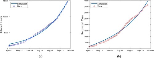
Table 1. Parameters value (2(2) $\begin{array}{rl}\mathrm{d}S\left(t\right)& =[\mathrm{\Pi }-{\mu }_{2}mX(t\left)S\right(t)-\eta S(t\left)I\right(t)-(\delta +d\left)S\right(t\left)\right]\mathrm{d}t\\ & +{\xi }_{1}S\left(t\right)\mathrm{d}{W}_1\left(t\right)\\ & +{\int }_Y{B}_1\left(y\right)S\left(t^{-}\right)\tilde{N}(\mathrm{d}t,\mathrm{d}y),\\ \mathrm{d}I\left(t\right)& =\left[\eta I\right(t\left)S\right(t)-(d+{\gamma }_1+{\mu }_1\left)I\right(t\left)\right]\mathrm{d}t+{\xi }_{2}I\left(t\right)\mathrm{d}{W}_2\left(t\right)\\ & +{\int }_Y{B}_2\left(y\right)I\left(t^{-}\right)\tilde{N}(\mathrm{d}t,\mathrm{d}y),\\ \mathrm{d}R\left(t\right)& =\left[{\gamma }_{1}I\right(t)+{\mu }_{2}mX(t\left)S\right(t)+\delta S(t)-\mathrm{d}R(t\left)\right]\mathrm{d}t+{\xi }_{3}R\left(t\right)\mathrm{d}{W}_3\left(t\right)\\ & +{\int }_Y{B}_3\left(y\right)R\left(t^{-}\right)\tilde{N}(\mathrm{d}t,\mathrm{d}y),\\ \mathrm{d}X\left(t\right)& =[\frac{{\mu }_{3}I\left(t\right)}{(1+hI(t\left)\right)}-aX(t\left)\right]\mathrm{d}t+{\xi }_{4}X\left(t\right)\mathrm{d}{W}_4\left(t\right)+{\int }_Y{B}_4\left(y\right)X\left(t^{-}\right)\tilde{N}(\mathrm{d}t,\mathrm{d}y),\end{array}$(2) ).

Parameter	Value	Source
Π	120.0166	Fitted
δ	6.6110	Fitted
η	0.1573	Fitted
d	4.37	Fitted
${\mu }_2$	0.212	Fitted
${\gamma }_1$	0.0081	Fitted
${\mu }_1$	0.4166	Fitted

6. Numerical simulations

To further verify the cogency of the theoretical analysis discussed above, in this part, we give some of the numerical simulation results. The theoretical results are illustrated numerically from two aspects: deterministic (model (1(1) $\begin{array}{rl}\frac{\mathrm{d}S\left(t\right)}{\mathrm{d}t}& =\mathrm{\Pi }-\eta S\left(t\right)I\left(t\right)-(\delta +d)S\left(t\right),\\ \frac{\mathrm{d}I\left(t\right)}{\mathrm{d}t}& =\eta I\left(t\right)S\left(t\right)-(d+{\gamma }_1+{\mu }_1)I\left(t\right),\\ \frac{\mathrm{d}R\left(t\right)}{\mathrm{d}t}& ={\gamma }_{1}I\left(t\right)+\delta S\left(t\right)-\mathrm{d}R\left(t\right).\end{array}$(1) )) and stochastic (model (2(2) $\begin{array}{rl}\mathrm{d}S\left(t\right)& =[\mathrm{\Pi }-{\mu }_{2}mX(t\left)S\right(t)-\eta S(t\left)I\right(t)-(\delta +d\left)S\right(t\left)\right]\mathrm{d}t\\ & +{\xi }_{1}S\left(t\right)\mathrm{d}{W}_1\left(t\right)\\ & +{\int }_Y{B}_1\left(y\right)S\left(t^{-}\right)\tilde{N}(\mathrm{d}t,\mathrm{d}y),\\ \mathrm{d}I\left(t\right)& =\left[\eta I\right(t\left)S\right(t)-(d+{\gamma }_1+{\mu }_1\left)I\right(t\left)\right]\mathrm{d}t+{\xi }_{2}I\left(t\right)\mathrm{d}{W}_2\left(t\right)\\ & +{\int }_Y{B}_2\left(y\right)I\left(t^{-}\right)\tilde{N}(\mathrm{d}t,\mathrm{d}y),\\ \mathrm{d}R\left(t\right)& =\left[{\gamma }_{1}I\right(t)+{\mu }_{2}mX(t\left)S\right(t)+\delta S(t)-\mathrm{d}R(t\left)\right]\mathrm{d}t+{\xi }_{3}R\left(t\right)\mathrm{d}{W}_3\left(t\right)\\ & +{\int }_Y{B}_3\left(y\right)R\left(t^{-}\right)\tilde{N}(\mathrm{d}t,\mathrm{d}y),\\ \mathrm{d}X\left(t\right)& =[\frac{{\mu }_{3}I\left(t\right)}{(1+hI(t\left)\right)}-aX(t\left)\right]\mathrm{d}t+{\xi }_{4}X\left(t\right)\mathrm{d}{W}_4\left(t\right)+{\int }_Y{B}_4\left(y\right)X\left(t^{-}\right)\tilde{N}(\mathrm{d}t,\mathrm{d}y),\end{array}$(2) )). We choose the time interval from 0 to 200, and the starting value of the $\left(\mathcal{S}\right(0),\mathcal{I}(0),\mathcal{R}(0),X(0\left)\right)$ is set as $(10,50,50,10)$ and $\mathrm{\Delta }=0.05$.

To ensure the validity of the model and satisfy the biological significance, the parameters and the noise intensity values are listed in Example 6.1. From Figure 2, a clear result is that when the value of basic regenerative number ${\mathcal{R}}_0^D<1$, a disease-free equilibrium point exists. Not only the solution trajectory of model (2(2) $\begin{array}{rl}\mathrm{d}S\left(t\right)& =[\mathrm{\Pi }-{\mu }_{2}mX(t\left)S\right(t)-\eta S(t\left)I\right(t)-(\delta +d\left)S\right(t\left)\right]\mathrm{d}t\\ & +{\xi }_{1}S\left(t\right)\mathrm{d}{W}_1\left(t\right)\\ & +{\int }_Y{B}_1\left(y\right)S\left(t^{-}\right)\tilde{N}(\mathrm{d}t,\mathrm{d}y),\\ \mathrm{d}I\left(t\right)& =\left[\eta I\right(t\left)S\right(t)-(d+{\gamma }_1+{\mu }_1\left)I\right(t\left)\right]\mathrm{d}t+{\xi }_{2}I\left(t\right)\mathrm{d}{W}_2\left(t\right)\\ & +{\int }_Y{B}_2\left(y\right)I\left(t^{-}\right)\tilde{N}(\mathrm{d}t,\mathrm{d}y),\\ \mathrm{d}R\left(t\right)& =\left[{\gamma }_{1}I\right(t)+{\mu }_{2}mX(t\left)S\right(t)+\delta S(t)-\mathrm{d}R(t\left)\right]\mathrm{d}t+{\xi }_{3}R\left(t\right)\mathrm{d}{W}_3\left(t\right)\\ & +{\int }_Y{B}_3\left(y\right)R\left(t^{-}\right)\tilde{N}(\mathrm{d}t,\mathrm{d}y),\\ \mathrm{d}X\left(t\right)& =[\frac{{\mu }_{3}I\left(t\right)}{(1+hI(t\left)\right)}-aX(t\left)\right]\mathrm{d}t+{\xi }_{4}X\left(t\right)\mathrm{d}{W}_4\left(t\right)+{\int }_Y{B}_4\left(y\right)X\left(t^{-}\right)\tilde{N}(\mathrm{d}t,\mathrm{d}y),\end{array}$(2) ) with Levy jump but also the stochastic epidemic model (2(2) $\begin{array}{rl}\mathrm{d}S\left(t\right)& =[\mathrm{\Pi }-{\mu }_{2}mX(t\left)S\right(t)-\eta S(t\left)I\right(t)-(\delta +d\left)S\right(t\left)\right]\mathrm{d}t\\ & +{\xi }_{1}S\left(t\right)\mathrm{d}{W}_1\left(t\right)\\ & +{\int }_Y{B}_1\left(y\right)S\left(t^{-}\right)\tilde{N}(\mathrm{d}t,\mathrm{d}y),\\ \mathrm{d}I\left(t\right)& =\left[\eta I\right(t\left)S\right(t)-(d+{\gamma }_1+{\mu }_1\left)I\right(t\left)\right]\mathrm{d}t+{\xi }_{2}I\left(t\right)\mathrm{d}{W}_2\left(t\right)\\ & +{\int }_Y{B}_2\left(y\right)I\left(t^{-}\right)\tilde{N}(\mathrm{d}t,\mathrm{d}y),\\ \mathrm{d}R\left(t\right)& =\left[{\gamma }_{1}I\right(t)+{\mu }_{2}mX(t\left)S\right(t)+\delta S(t)-\mathrm{d}R(t\left)\right]\mathrm{d}t+{\xi }_{3}R\left(t\right)\mathrm{d}{W}_3\left(t\right)\\ & +{\int }_Y{B}_3\left(y\right)R\left(t^{-}\right)\tilde{N}(\mathrm{d}t,\mathrm{d}y),\\ \mathrm{d}X\left(t\right)& =[\frac{{\mu }_{3}I\left(t\right)}{(1+hI(t\left)\right)}-aX(t\left)\right]\mathrm{d}t+{\xi }_{4}X\left(t\right)\mathrm{d}{W}_4\left(t\right)+{\int }_Y{B}_4\left(y\right)X\left(t^{-}\right)\tilde{N}(\mathrm{d}t,\mathrm{d}y),\end{array}$(2) ) approaches to the disease-free equilibrium point of its deterministic version, representing that the disease approaches to be extinct. Theorem 3.1 presents the sufficient condition for extinction of model (2(2) $\begin{array}{rl}\mathrm{d}S\left(t\right)& =[\mathrm{\Pi }-{\mu }_{2}mX(t\left)S\right(t)-\eta S(t\left)I\right(t)-(\delta +d\left)S\right(t\left)\right]\mathrm{d}t\\ & +{\xi }_{1}S\left(t\right)\mathrm{d}{W}_1\left(t\right)\\ & +{\int }_Y{B}_1\left(y\right)S\left(t^{-}\right)\tilde{N}(\mathrm{d}t,\mathrm{d}y),\\ \mathrm{d}I\left(t\right)& =\left[\eta I\right(t\left)S\right(t)-(d+{\gamma }_1+{\mu }_1\left)I\right(t\left)\right]\mathrm{d}t+{\xi }_{2}I\left(t\right)\mathrm{d}{W}_2\left(t\right)\\ & +{\int }_Y{B}_2\left(y\right)I\left(t^{-}\right)\tilde{N}(\mathrm{d}t,\mathrm{d}y),\\ \mathrm{d}R\left(t\right)& =\left[{\gamma }_{1}I\right(t)+{\mu }_{2}mX(t\left)S\right(t)+\delta S(t)-\mathrm{d}R(t\left)\right]\mathrm{d}t+{\xi }_{3}R\left(t\right)\mathrm{d}{W}_3\left(t\right)\\ & +{\int }_Y{B}_3\left(y\right)R\left(t^{-}\right)\tilde{N}(\mathrm{d}t,\mathrm{d}y),\\ \mathrm{d}X\left(t\right)& =[\frac{{\mu }_{3}I\left(t\right)}{(1+hI(t\left)\right)}-aX(t\left)\right]\mathrm{d}t+{\xi }_{4}X\left(t\right)\mathrm{d}{W}_4\left(t\right)+{\int }_Y{B}_4\left(y\right)X\left(t^{-}\right)\tilde{N}(\mathrm{d}t,\mathrm{d}y),\end{array}$(2) ). The numerical simulation results show that the outcomes of Theorem 3.1 will be held if and only if ${\mathcal{R}}_0<1$.

Figure 2. The trajectories of stochastic system (2(2) $\begin{array}{rl}\mathrm{d}S\left(t\right)& =[\mathrm{\Pi }-{\mu }_{2}mX(t\left)S\right(t)-\eta S(t\left)I\right(t)-(\delta +d\left)S\right(t\left)\right]\mathrm{d}t\\ & +{\xi }_{1}S\left(t\right)\mathrm{d}{W}_1\left(t\right)\\ & +{\int }_Y{B}_1\left(y\right)S\left(t^{-}\right)\tilde{N}(\mathrm{d}t,\mathrm{d}y),\\ \mathrm{d}I\left(t\right)& =\left[\eta I\right(t\left)S\right(t)-(d+{\gamma }_1+{\mu }_1\left)I\right(t\left)\right]\mathrm{d}t+{\xi }_{2}I\left(t\right)\mathrm{d}{W}_2\left(t\right)\\ & +{\int }_Y{B}_2\left(y\right)I\left(t^{-}\right)\tilde{N}(\mathrm{d}t,\mathrm{d}y),\\ \mathrm{d}R\left(t\right)& =\left[{\gamma }_{1}I\right(t)+{\mu }_{2}mX(t\left)S\right(t)+\delta S(t)-\mathrm{d}R(t\left)\right]\mathrm{d}t+{\xi }_{3}R\left(t\right)\mathrm{d}{W}_3\left(t\right)\\ & +{\int }_Y{B}_3\left(y\right)R\left(t^{-}\right)\tilde{N}(\mathrm{d}t,\mathrm{d}y),\\ \mathrm{d}X\left(t\right)& =[\frac{{\mu }_{3}I\left(t\right)}{(1+hI(t\left)\right)}-aX(t\left)\right]\mathrm{d}t+{\xi }_{4}X\left(t\right)\mathrm{d}{W}_4\left(t\right)+{\int }_Y{B}_4\left(y\right)X\left(t^{-}\right)\tilde{N}(\mathrm{d}t,\mathrm{d}y),\end{array}$(2) ) and its corresponding deterministic systems for Example 6.1. (a) Susceptible population, (b) infected population, (c) recovered population and (d) information in the population.

Example 6.1

In this example, the parameters are $\mathrm{\Pi }=4.80$, $\delta =0.58$, $\eta =0.03$, d = 0.02, ${\mu }_2=0.4$, m = 0.4,${\gamma }_1=0.20$, ${\mu }_1=0.02$, ${\mu }_3=0.10$, h = 2.00, a = 0.20, and the noise intensities assumed are ${\xi }_1=0.55$, ${\xi }_2=0.40$, ${\xi }_3=0.30$, ${\xi }_4=0.20$, and $B_{\iota }\left(\mathrm{{\rm Y}}\right)=-k_{i}B\left(\mathrm{{\rm Y}}\right)/(1+B(\mathrm{{\rm Y}}{)}^2),\mathrm{{\rm Y}}=0.5$, with $k_1=0.45$, $k_2=0.45$, $k_3=0.04$, $k_4=0.03$. The basic fertility rate ${\mathcal{R}}_{\mathbf{0}}^{\mathbf{D}}<1$ as well as the stochastic threshold ${\mathcal{R}}_{\mathbf{0}}<1$ are simple to compute. The epidemic will become extinct, as per Theorem 3.1. The extinction of the epidemic is well noticed in the stochastic system's path in Figure 2(a–d).

In addition, we verify the persistence of the disease numerically and we take the parameters from Example 6.2 in a stochastic version. Under the condition, we calculate that the basic regenerative number ${\mathcal{R}}_{\mathbf{0}}^{\mathbf{D}}>1$, also ${\mathcal{R}}_0^s>1$, which implies that Theorem 4.1 is fulfilled. Under the influence of the weak noise, the epidemic will still remain. As shown in Figure 3(a–d), the epidemic model (2(2) $\begin{array}{rl}\mathrm{d}S\left(t\right)& =[\mathrm{\Pi }-{\mu }_{2}mX(t\left)S\right(t)-\eta S(t\left)I\right(t)-(\delta +d\left)S\right(t\left)\right]\mathrm{d}t\\ & +{\xi }_{1}S\left(t\right)\mathrm{d}{W}_1\left(t\right)\\ & +{\int }_Y{B}_1\left(y\right)S\left(t^{-}\right)\tilde{N}(\mathrm{d}t,\mathrm{d}y),\\ \mathrm{d}I\left(t\right)& =\left[\eta I\right(t\left)S\right(t)-(d+{\gamma }_1+{\mu }_1\left)I\right(t\left)\right]\mathrm{d}t+{\xi }_{2}I\left(t\right)\mathrm{d}{W}_2\left(t\right)\\ & +{\int }_Y{B}_2\left(y\right)I\left(t^{-}\right)\tilde{N}(\mathrm{d}t,\mathrm{d}y),\\ \mathrm{d}R\left(t\right)& =\left[{\gamma }_{1}I\right(t)+{\mu }_{2}mX(t\left)S\right(t)+\delta S(t)-\mathrm{d}R(t\left)\right]\mathrm{d}t+{\xi }_{3}R\left(t\right)\mathrm{d}{W}_3\left(t\right)\\ & +{\int }_Y{B}_3\left(y\right)R\left(t^{-}\right)\tilde{N}(\mathrm{d}t,\mathrm{d}y),\\ \mathrm{d}X\left(t\right)& =[\frac{{\mu }_{3}I\left(t\right)}{(1+hI(t\left)\right)}-aX(t\left)\right]\mathrm{d}t+{\xi }_{4}X\left(t\right)\mathrm{d}{W}_4\left(t\right)+{\int }_Y{B}_4\left(y\right)X\left(t^{-}\right)\tilde{N}(\mathrm{d}t,\mathrm{d}y),\end{array}$(2) ) will persist around average value of the disease which verify the outcomes of Theorem 4.1.

Figure 3. The trajectories of stochastic system (2(2) $\begin{array}{rl}\mathrm{d}S\left(t\right)& =[\mathrm{\Pi }-{\mu }_{2}mX(t\left)S\right(t)-\eta S(t\left)I\right(t)-(\delta +d\left)S\right(t\left)\right]\mathrm{d}t\\ & +{\xi }_{1}S\left(t\right)\mathrm{d}{W}_1\left(t\right)\\ & +{\int }_Y{B}_1\left(y\right)S\left(t^{-}\right)\tilde{N}(\mathrm{d}t,\mathrm{d}y),\\ \mathrm{d}I\left(t\right)& =\left[\eta I\right(t\left)S\right(t)-(d+{\gamma }_1+{\mu }_1\left)I\right(t\left)\right]\mathrm{d}t+{\xi }_{2}I\left(t\right)\mathrm{d}{W}_2\left(t\right)\\ & +{\int }_Y{B}_2\left(y\right)I\left(t^{-}\right)\tilde{N}(\mathrm{d}t,\mathrm{d}y),\\ \mathrm{d}R\left(t\right)& =\left[{\gamma }_{1}I\right(t)+{\mu }_{2}mX(t\left)S\right(t)+\delta S(t)-\mathrm{d}R(t\left)\right]\mathrm{d}t+{\xi }_{3}R\left(t\right)\mathrm{d}{W}_3\left(t\right)\\ & +{\int }_Y{B}_3\left(y\right)R\left(t^{-}\right)\tilde{N}(\mathrm{d}t,\mathrm{d}y),\\ \mathrm{d}X\left(t\right)& =[\frac{{\mu }_{3}I\left(t\right)}{(1+hI(t\left)\right)}-aX(t\left)\right]\mathrm{d}t+{\xi }_{4}X\left(t\right)\mathrm{d}{W}_4\left(t\right)+{\int }_Y{B}_4\left(y\right)X\left(t^{-}\right)\tilde{N}(\mathrm{d}t,\mathrm{d}y),\end{array}$(2) ) and its corresponding deterministic systems for Example 6.2. (a) Susceptible population, (b) infected population, (c) recovered population and (d) information in the population.

Example 6.2

In this example, the parameters are $\mathrm{\Pi }=2$, $\delta =0.05$, $\eta =0.09$, d = 0.02, ${\mu }_2=0.5$, m = 0.01,${\gamma }_1=0.2$, ${\mu }_1=0.02$, ${\mu }_3=0.5$, h = 1, a = 0.02, and the noise intensities assumed are ${\xi }_1=0.5$, ${\xi }_2=0.4$, ${\xi }_3=0.05$, ${\xi }_4=0.05$, and $B_{\iota }\left(\mathrm{{\rm Y}}\right)=-k_{i}B\left(\mathrm{{\rm Y}}\right)/(1+B(\mathrm{{\rm Y}}{)}^2),\mathrm{{\rm Y}}=0.5$, where $k_1=0.5$, $k_2=0.4$, $k_3=0.05$, $k_4=0.05$. We can calculate easily the basic reproduction rate ${\mathcal{R}}_{\mathbf{0}}^{\mathbf{D}}>1$ and the stochastic threshold ${\mathcal{R}}_{\mathbf{0}}^{\mathbf{s}}>1$ which will persist in mean which support the conclusion of Theorem 4.1.

Example 6.3

In this example, we keep the same parameters as Example 6.2 and we change the noise intensities ${\xi }_1=0.7$, ${\xi }_2=0.5$, ${\xi }_3=0.05$, ${\xi }_4=0.06$, $B_{\iota }\left(\mathrm{{\rm Y}}\right)=-k_{i}B\left(\mathrm{{\rm Y}}\right)/(1+B(\mathrm{{\rm Y}}{)}^2),\mathrm{{\rm Y}}=0.5$, where $k_1=0.6$, $k_2=0.45$, $k_3=0.03$, $k_4=0.04$. We can calculate easily the basic reproduction rate ${\mathcal{R}}_{\mathbf{0}}^{\mathbf{D}}>1$ and the stochastic threshold ${\mathcal{R}}_{\mathbf{0}}^{\mathbf{s}}>1$. As observed in Figure 4, the disease will persist in mean which support the conclusion of Theorem 4.1 (see Figure 4(a–d)).

Figure 4. The trajectories of the stochastic system (2(2) $\begin{array}{rl}\mathrm{d}S\left(t\right)& =[\mathrm{\Pi }-{\mu }_{2}mX(t\left)S\right(t)-\eta S(t\left)I\right(t)-(\delta +d\left)S\right(t\left)\right]\mathrm{d}t\\ & +{\xi }_{1}S\left(t\right)\mathrm{d}{W}_1\left(t\right)\\ & +{\int }_Y{B}_1\left(y\right)S\left(t^{-}\right)\tilde{N}(\mathrm{d}t,\mathrm{d}y),\\ \mathrm{d}I\left(t\right)& =\left[\eta I\right(t\left)S\right(t)-(d+{\gamma }_1+{\mu }_1\left)I\right(t\left)\right]\mathrm{d}t+{\xi }_{2}I\left(t\right)\mathrm{d}{W}_2\left(t\right)\\ & +{\int }_Y{B}_2\left(y\right)I\left(t^{-}\right)\tilde{N}(\mathrm{d}t,\mathrm{d}y),\\ \mathrm{d}R\left(t\right)& =\left[{\gamma }_{1}I\right(t)+{\mu }_{2}mX(t\left)S\right(t)+\delta S(t)-\mathrm{d}R(t\left)\right]\mathrm{d}t+{\xi }_{3}R\left(t\right)\mathrm{d}{W}_3\left(t\right)\\ & +{\int }_Y{B}_3\left(y\right)R\left(t^{-}\right)\tilde{N}(\mathrm{d}t,\mathrm{d}y),\\ \mathrm{d}X\left(t\right)& =[\frac{{\mu }_{3}I\left(t\right)}{(1+hI(t\left)\right)}-aX(t\left)\right]\mathrm{d}t+{\xi }_{4}X\left(t\right)\mathrm{d}{W}_4\left(t\right)+{\int }_Y{B}_4\left(y\right)X\left(t^{-}\right)\tilde{N}(\mathrm{d}t,\mathrm{d}y),\end{array}$(2) ) and its corresponding deterministic systems for Example 6.2, with various relapse rate $({\xi }_1,{\xi }_2,{\xi }_3,{\xi }_4)=(0.7,0.5,0.02,0.06)$ and $B_i\left(y\right)=-k_{i}B\left(y\right)/(1+B(y{)}^2),y=0.5$ where $(k_1,k_2,k_3,k_4)=(0.6,0.45,0.03,0.04)$. (a) Susceptible population, (b) infected population, (c) recovered population and (d) information in the population.

7. Conclusion

This work focuses on investigating the dynamic of stochastic SIR model about COVID-19 with the influence of information intervention and Lévy noise, under real statistic data. First, we investigate the existence and uniqueness of a global positive solution of the proposed model driven by the Levy noise. Second, using the Lyapunov technique, it is concluded that the solution fluctuates around the equilibrium point within reasonable range of chosen parameters. Third, an empirical analysis corresponding to the COVID-19 disease data from 13 April 2020 to 1 October 2020 in Pakistan has been presented for validation. In addition, illustrating by the numerical result, the population fluctuation of the different types of infected individual has been presented. We deduced that the relapse rate and recovery rate also have intense impacts on the magnitude of the infected individuals. It can be concluded that the role of influence of information intervention and Lévy noise reduces the disease transmission rate. In a future work, we will focus on the stochastic model with vaccination.

Authors' contribution

All authors have equal contribution.

Disclosure statement

No potential conflict of interest was reported by the author(s).

Additional information

Funding

This work was supported by the National Natural Science Foundation of P. R. China (Grant Nos. 11901114 and 11801073), Guangzhou Science and Technology Innovation general project (Grant No. 201904010010), Young Innovative Talents Project of Guangdong Provincial Department of Education (Grant No. 2017KQNCX081) and Natural Science Foundation of Guangdong Province (Grant No. 2017A030310598).

References

- L.J.S. Allen, B.M. Bolker, Y. Lou, and A.L. Nevai, Asymptotic profiles of the steady states for an SIS epidemic reaction-diffusion model, Discrete Contin. Dyn. Syst. A 21(1) (2008), Article ID 1.
- A. Atangana and S. İğret Araz, Modeling and forecasting the spread of COVID-19 with stochastic and deterministic approaches: Africa and Europe, Adv. Differ. Equ. 2021(1) (2021), pp. 1–107.
- K. Bao and Q. Zhang, Stationary distribution and extinction of a stochastic SIRS epidemic model with information intervention, Adv. Differ. Equ. 2017(1) (2017), pp. 1–19.
- J.R. Beddington and R.M. May, Harvesting natural populations in a randomly fluctuating environment, Science 197(4302) (1977), pp. 463–465.
- B.-E. Berrhazi, M. El Fatini, T. Caraballo Garrido, and R. Pettersson, A stochastic SIRI epidemic model with Lévy noise, Discrete Contin. Dyn. Syst. Ser. B 23(9) (2018), pp. 3645–3661.
- A. Din, Y. Li, T. Khan, and G. Zaman, Mathematical analysis of spread and control of the novel corona virus (COVID-19) in China, Chaos Solitons Fractals 141 (2020), Article ID 110286.
- A. Din, Y. Li, and A. Yusuf, Delayed hepatitis B epidemic model with stochastic analysis, Chaos Solitons Fractals 146 (2021), Article ID 110839.
- A. Din and Y. Li, The complex dynamics of hepatitis B infected individuals with optimal control, J. Syst. Sci. Complex 33 (2020), pp. 1–23.
- A. Din and Y. Li, Lévy noise impact on a stochastic hepatitis B epidemic model under real statistical data and its fractal–fractional Atangana–Baleanu order model, Phys. Scr. 95 (2021), pp. 1–17.
- A. Din and Y. Li, Stationary distribution extinction and optimal control for the stochastic hepatitis B epidemic model with partial immunity, Phys. Scr. 69 (2021), pp. 1–29.
- Y. Ding, M. Xu, and L. Hu, Asymptotic behavior and stability of a stochastic model for AIDS transmission, Appl. Math. Comput. 204(1) (2008), pp. 99–108.
- Y. Dong and T. Lin, Dynamics of a stochastic rumor propagation model incorporating media coverage and driven by Lévy noise, Chin. Phys. B 30 (2021), pp. 2–10.
- M. El Fatini and I. Sekkak, Lévy noise impact on a stochastic delayed epidemic model with Crowly–Martin incidence and crowding effect, Physica A 541 (2020), Article ID 123315.
- R. Gao, B. Cao, Y. Hu, Z. Feng, D. Wang, W. Hu, J. Chen, Z. Jie, H. Qiu, K. Xu, and X. Xu, Human infection with a novel avian-origin influenza A (H7N9) virus, N. Engl. J. Med. 368(20) (2013), pp. 1888–1897.
- Q. Han, D. Jiang, and C. Ji, Analysis of a delayed stochastic predator–prey model in a polluted environment, Appl. Math. Model. 38(13) (2014), pp. 3067–3080.
- T. Khan, A. Khan, and G. Zaman, The extinction and persistence of the stochastic hepatitis B epidemic model, Chaos Solitons Fractals 108 (2018), pp. 123–128.
- T. Khan, G. Zaman, and M. Ikhlaq Chohan, The transmission dynamic and optimal control of acute and chronic hepatitis B, J. Biol. Dyn. 11(1) (2017), pp. 172–189.
- S. Nana-Kyere, J. Ackora-Prah, E. Okyere, S. Marmah, and T. Afram, Hepatitis B optimal control model with vertical transmission, Appl. Math. 7(1) (2017), pp. 5–13.
- S.A. Trigger and E.B. Czerniawski, Equation for epidemic spread with the quarantine measures: application to COVID-19, Phys. Scr. 95(10) (2020), Article ID 105001.
- T.M. Uyeki and N.J. Cox, Global concerns regarding novel influenza A (H7N9) virus infections, N. Engl. J. Med. 368(20) (2013), pp. 1862–1864.
- A. Yousefpour, H. Jahanshahi, and S. Bekiros, Optimal policies for control of the novel coronavirus disease (COVID-19) outbreak, Chaos Solitons Fractals 136 (2020), Article ID 109883.
- L. Zhu, X. Wang, H. Zhang, S. Shen, Y. Li, and Y. Zhou, Dynamics analysis and optimal control strategy for a SIRS epidemic model with two discrete time delays, Phys. Scr. 95(3) (2020), Article ID 035213.