The effect of spatial dynamics on the behaviour of an environmentally transmitted disease

Abstract

Understanding the spread of pathogens through the environment is critical to a fuller comprehension of disease dynamics. However, many mathematical models of disease dynamics ignore spatial effects. We seek to expand knowledge around the interaction between the bare-nosed wombat (Vombatus ursinus) and sarcoptic mange (etiologic agent Sarcoptes scabiei), by extending an aspatial mathematical model to include spatial variation. S. scabiei was found to move through our modelled region as a spatio-temporal travelling wave, leaving behind pockets of localized host extinction, consistent with field observations. The speed of infection spread was also comparable with field research. Our model predicts that the inclusion of spatial dynamics leads to the survival and recovery of affected wombat populations when an aspatial model predicts extinction. Collectively, this research demonstrates how environmentally transmitted S. scabiei can result in travelling wave dynamics, and that inclusion of spatial variation reveals a more resilient host population than aspatial modelling approaches.

Keywords:

• Scabies
• pathogen spread
• common wombat
• landscape epidemiology
• environmental transmission

1. Introduction

Characterizing the spread of pathogens through the environment has important consequences for understanding disease dynamics [1]. In nature, there are a range of spatial patterns that are recognized with disease spread [21, 29, 37], such as a unidirectional travelling wave [19], spatial jumps between local spread [21, 33], spread moving back and forth between populations [9] and spatially heterogeneous incidence, e.g. stuttering chains [8]. Varying mechanisms of transmission can influence the types of spatial dynamics observed [18]. For example, large spatial jumps may be observed for direct transmission associated with dispersal events [17, 33] and travelling waves may be common where transmission is dependent on contact with environmental fomites [26]. Thus spatial dynamics are important [6, 26, 43], but it is less common for them to be explicitly included in models of disease dynamics [32].

Some of the most conservation critical diseases impacting wildlife include environmental transmission [4, 11, 42] and understanding their spread can help guide epidemiological understanding and management. Important examples include chytridiomycosis in amphibians [42], White Nose Syndrome in bats [15] and sarcoptic mange [26]. All of these diseases are caused by pathogens that can drive population declines and, in some cases, extinction events [15, 26, 42]. Examples of spatial disease dynamics among these systems have included both travelling waves [13, 19, 26, 37] and larger spatial jumps [24]. Travelling waves, when they are documented, are generally characterized at local scales within host species [26].

Sarcoptic mange is one of the most host-generalist and impactful of mammalian parasites [4]. The parasitic mite causing sarcoptic mange (also known as scabies in humans), Sarcoptes scabiei is known to infect over 100 mammalian species throughout diverse regions globally [30]. This skin infection causes a range of pathological outcomes including pruritus, alopecia, secondary bacterial infections and emaciation [2]. The disease is known to cause epizootics [30], host population declines [30] and extirpation events [30] among host species. It has an expanding host species range and is considered an emerging infectious disease in some mammals [40]. Further, scabies is among the 30 most prevalent human diseases [44], with approximately 200 million cases at any one time [44]. It was recently classified as a Neglected Tropical Disease by the World Health Organisation [20].

The most important disease impacting bare-nosed wombats (Vombatus ursinus) is sarcoptic mange [26] which, in this case, is environmentally transmitted [35]. Wombats tend to suffer severely, developing crusted mange after infection and eventually perishing unless treated [26, 34]. Infection can lead to a range of population outcomes, including epizootics with population decline [26, 35], and stable population and disease dynamics [12]. Evidence suggests S. scabiei was introduced to Australia by European settlers and their domestic animals [14, 35]. On a local scale, mange is understood to spread through wombat populations via the asynchronous sharing of burrows [35]. Empirical evidence suggests local spread can occur as a travelling wave [26] and several models of dynamics now exist, but the inclusion of spatial dynamics is lacking [6, 7, 27].

In this study, we seek to characterize the spatial dynamics and spatial behaviour of an outbreak of S. scabiei on wombat populations. We seek to expand upon the findings of a spatially homogeneous model explored by Beeton et al. [6], as seen in Figure 1, with a spatially inhomogeneous model. Beeton et al. [6] found that under a moderate rate of transmission ($\beta =0.05$) that wombat populations tended to extinction or near-extinction following mite introduction under a range of biologically plausible parameters (such as mite shedding rates f and fomite survival times in the environment ${\mu }_F$) yet, as described above, wombat populations often persist with mange. Of course, an acknowledged limitation of spatially homogenous models are assumptions of equal mixing in space, whereas space and animal movement play important roles in infection risk in nature. Thus, using plausible biological conditions evaluated in [6], we seek to establish how this disease moves throughout a region occupied by bare-nosed wombats and describe characteristics of that pattern. We hypothesize that mange will spread in a wave pattern, consistent with empirical observations [26], but that the specific inclusion of spatial dynamics in the model will accommodate biological features that may support population persistence.

Figure 1. A modified version of the model seen in [6]. Here the transmission method is indirect and the population of the mites is modelled explicitly to represent this indirect transmission. Here, S are the susceptible wombats, $I_L$ are asymptomatic carriers of the disease, $I_H$ are symptomatic infected wombats, F are the fomites existing in the environment, b is the birth rate of wombats, μ is the death rate without infection of wombats, ${\mu }_L$ is the death rate due to asymptomatic infection, ${\mu }_H$ is the death rate due to symptomatic infection, β is the rate at which susceptible wombats are infected, γ is the rate at which asymptomatic wombats become symptomatic, f is the rate that infected wombats drop fomites into the environment and ${\mu }_F$ is the rate that fomites within the environment die.

2. The model

A conceptual model illustrating the wombat-mite system and its dynamics is illustrated in Figure 1, with rate parameters for the system described in Table 1. See below for the description of wombat and fomite populations within the model, and beginning of the results for the description of the simulations investigated.

Table 1. Rate parameters for the PDE (see equations (1(1) $\begin{array}{rl}\frac{\mathrm{\partial }S}{\mathrm{\partial }t}& =\sigma {\mathrm{\nabla }}^{2}S+bN(1-N)-\frac{\beta SF}{1+F}-\mu S,\end{array}$(1) )–(4(4) $\begin{array}{rl}\frac{\mathrm{\partial }F}{\mathrm{\partial }t}& =f(I_L+I_H)-{\mu }_{F}F.\end{array}$(4) ) and Figure 1) describing transmission of S. scabiei among wombats.

Parameter	Symbol	Values	Source
Wombat spatial diffusion rate	σ	$1/(1.5\times 365\times 0.5\times 0.5)$	[5]
Wombat birth rate	b	$1/(3\times 365)$	[6, 27, 41]
Nonlinear disease spread rate	β	0.05	[6]
Wombat death rate	μ	$1/(15\times 365)$	[41]
Disease progression rate	γ	1/30	[27, 34]
Exposed wombat death rate	${\mu }_L$	1/60	[27]
Infected wombat death rate	${\mu }_H$	1/60	[27]
Mite drop rate	f	1/10	[6]
Mite death rate	${\mu }_F$	1/7,1/19	[2, 3, 10]

Note: All rates are in days, and the wombat spatial diffusion rate is in km/day.

We create a system of nonlinear equations in two spatial dimensions and time, based on the work of Beeton et al. [6]. The governing partial differential equations (PDEs) are (1) $\begin{array}{rl}\frac{\mathrm{\partial }S}{\mathrm{\partial }t}& =\sigma {\mathrm{\nabla }}^{2}S+bN(1-N)-\frac{\beta SF}{1+F}-\mu S,\end{array}$(1) (2) $\begin{array}{rl}\frac{\mathrm{\partial }{I}_L}{\mathrm{\partial }t}& =\sigma {\mathrm{\nabla }}^2{I}_L+\frac{\beta SF}{1+F}-(\mu +\gamma +{\mu }_L)I_L,\end{array}$(2) (3) $\begin{array}{rl}\frac{\mathrm{\partial }{I}_H}{\mathrm{\partial }t}& =\sigma {\mathrm{\nabla }}^2{I}_H+\gamma I_L-(\mu +{\mu }_H)I_H,\end{array}$(3) (4) $\begin{array}{rl}\frac{\mathrm{\partial }F}{\mathrm{\partial }t}& =f(I_L+I_H)-{\mu }_{F}F.\end{array}$(4) The ${\mathrm{\nabla }}^2$ operator used in the above equations refers to the two-dimensional Laplacian operator, which can be expanded as the sum of two partial second derivatives as follows: (5) ${\mathrm{\nabla }}^{2}S=\frac{{\mathrm{\partial }}^{2}S}{\mathrm{\partial }{x}^2}+\frac{{\mathrm{\partial }}^{2}S}{\mathrm{\partial }{y}^2}.$(5) This operator represents the movement of wombats throughout the system, and the movement is modelled as a diffusion process, with wombats spreading throughout the region at each time step.

The population of wombats that is being considered is split up and structured into subclasses, similar to the conventional SIR models of disease spread [22] and we label the sum of these subclasses as N, the total population. The subgroups that we consider are denoted as S, $I_L$ and $I_H$, corresponding to the following definitions: the subgroup S denotes the population that is susceptible to, but not currently infected by the S. scabiei parasite. The subgroup $I_L$ refers to the population of wombats that are asymptomatic carriers of the disease, wombats who have a low population of mites inhabiting them, such that they are not visibly exhibiting gross signs of pathology and cannot be detected as diseased in standard field studies . However, the wombats can potentially spread the mites in this stage. Subpopulation $I_H$ refers to wombats who show open signs of sarcoptic mange infection, have high populations of mites inhabiting them and can be readily detected in field studies, aligning closely with the classical definition of the infected subpopulation in disease modelling. The final class that we model is denoted by F, and is the fomite population, mites that survive in the bedding chamber of wombat burrows [6, 26]. Modelling the population of fomites is used as a proxy for the indirect transmission of sarcoptic mange in wombat populations. For the transmission function $(\beta SF)/(1+F),$ we assume an asymptotic effect of fomites, in that as mites increase within wombat burrows the effect of additional mites on infection risk diminishes (frequency-dependent transmission). This is consistent with our understanding of mange transmission among wombats [6, 27, 39]. The quantity $F/(1+F)$ is a self-limiting infection function, with 1 the non-dimensional limit as $F\to \mathrm{\infty }$. The quantity of fomites will lead to a maximum infection rate of $0.5\beta$ [6].

Importantly, we consider a barrier around the region which impedes the travel of the wombats. Physically, we could consider a reserve that has been fenced in or had natural barriers in place to impede movement (e.g. hills, rivers, dense forest, ocean, etc.). Mathematically, we use a set of boundary conditions given by (6) $\frac{\mathrm{\partial }N}{\mathrm{\partial }x}=0$(6) along the boundaries running orthogonal to the x-axis, and (7) $\frac{\mathrm{\partial }N}{\mathrm{\partial }y}=0$(7) along the boundaries running orthogonal to the y-axis. We can then impose an initial condition that is appropriate to the physical situation we wish to model.

With regard to the parameters in our model (Table 1), the reasoning for these is as follows: the wombat spatial diffusion rate is females relocating after successfully rearing a joey, approximately half a kilometre [5]; the wombat birth rate is one joey per female per 1.5 years; the transmission rate is consistent with Beeton et al. [6]; the death rate is based on a wombat lifespan of 15 years; the disease progression rate is a 30-day window before symptoms become clinically visible ($I_L$ moves to $I_H$); the death rate associated with mange is 60 days when showing clinical signs (thus infection to mortality = 90 days); the mite drop rate is consistent with Beeton et al. [6]; and the environmental mite death rates are for under optimal and sub-optimal environmental conditions (19 and 7 days, respectively).

3. Linearized stability

To understand how stable the populations $(S,I_L,I_H,F)$ are when they reach equilibrium (steady states), we approximated the system linearly and assessed it analytically. This is of value to understand how the equilibria we estimate (for which some parts we know are unstable in spatially homogenous populations) is influenced by the size of the area (number of modes) we specify in our study. This analysis is done by making a small perturbation to each of the populations around an equilibrium point, in the form $S=S_{\mathrm{eq}}+\epsilon S_1(x,y,t)+O({\epsilon }^2)$, with each of the populations being perturbed in an equivalent manner. Here, ε is a small parameter that represents the amplitude of a disturbance to the equilibrium state. To first order in ε, this gives the following linearized system of equations expanded upon in Appendix: (8) $\begin{array}{rl}\frac{\mathrm{\partial }{S}_1}{\mathrm{\partial }t}& =\sigma {\mathrm{\nabla }}^2{S}_1+b{N}_1(1-2N_{\mathrm{eq}})-\mu S_1-\frac{\beta F_{\mathrm{eq}}{S}_1}{1+F_{\mathrm{eq}}}+\frac{\beta S_{\mathrm{eq}}{F}_1}{(1+F_{\mathrm{eq}}{)}^2},\end{array}$(8) (9) $\begin{array}{rl}\frac{\mathrm{\partial }{I}_{L1}}{\mathrm{\partial }t}& =\sigma {\mathrm{\nabla }}^2{I}_{L1}+\frac{\beta F_{\mathrm{eq}}{S}_1}{1+F_{\mathrm{eq}}}+\frac{\beta S_{\mathrm{eq}}{F}_1}{(1+F_{\mathrm{eq}}{)}^2}-(\mu +\gamma +{\mu }_L)I_{L1},\end{array}$(9) (10) $\begin{array}{rl}\frac{\mathrm{\partial }{I}_{H1}}{\mathrm{\partial }t}& =\sigma {\mathrm{\nabla }}^2{I}_{H1}+\gamma I_{L1}-(\mu +{\mu }_H)I_{H1},\end{array}$(10) (11) $\begin{array}{rl}\frac{\mathrm{\partial }{F}_1}{\mathrm{\partial }t}& =f(E_1+I_1)-{\mu }_F{F}_1.\end{array}$(11) These linearized equations can then be used to assess local behaviour about equilibrium points. Specifically, we model each of the perturbed wombat populations by the following relation: (12) $S_1(x,y,t)=\sum _{n=0}^{\mathrm{\infty }}\sum _{m=0}^{\mathrm{\infty }}\sin \left(\frac{n\pi x}{L}\right)\sin \left(\frac{m\pi y}{B}\right)S_{mn}(t),$(12) where the parameters m and n are the modes of the solution. L represents half of the length of the region that we are studying, and parameter B represents half of the depth. A similar representation exists for the other variables. For convenience, we now define constants (13) $\begin{array}{rl}{Z}_{mn}^2& =\sigma [{\left(\frac{n\pi }{L}\right)}^2+{\left(\frac{m\pi }{B}\right)}^2],\end{array}$(13) (14) $\begin{array}{rl}{m}_H& =\mu +{\mu }_H,\end{array}$(14) (15) $\begin{array}{rl}{m}_L& =\mu +{\mu }_L,\end{array}$(15) (16) $\begin{array}{rl}{\mathrm{\Lambda }}_b& =b(1-2N_{\mathrm{eq}}).\end{array}$(16) Utilizing the above relations we can transform the linear equations into matrix form as (17) $\frac{\mathrm{\partial }{\overrightarrow{V}}_{mn}}{\mathrm{\partial }t}=J\cdot {\overrightarrow{V}}_{mn}.$(17) Here ${\overrightarrow{V}}_{mn}$ is the vector of perturbed Fourier coefficients at each set of modes $(m,n)$. It is represented here as (18) ${\overrightarrow{V}}_{mn}={\left[\begin{array}{c}{S}_1\\ I_{L1}\\ I_{H1}\\ F_1\end{array}\right]}_{mn}.$(18) The symbol J represents the Jacobian matrix: (19) $J=\left[\begin{array}{cccc}-Z_{mn}^2-\mu -K_1+{\mathrm{\Lambda }}_b& {\mathrm{\Lambda }}_b& {\mathrm{\Lambda }}_b& -K_2\\ \\ K_1& -Z_{mn}^2-(m_L+\gamma )& 0& K_2\\ \\ 0& \gamma & -Z_{mn}^2-m_H& 0\\ \\ 0& f& f& -{\mu }_F\end{array}\right],$(19) where we have defined the two additional intermediate constants $K_1={\displaystyle \frac{\beta F_{\mathrm{eq}}}{1+F_{\mathrm{eq}}}}$and $K_2={\displaystyle \frac{\beta S_{\mathrm{eq}}}{(1+F_{\mathrm{eq}}{)}^2}}.$The equilibrium point of primary interest is the case where only wombats exist in the system, thus allowing us to perturb the Mite population slightly and assess the evolving dynamics. This is represented as (20) $(S,I_L,I_H,F{)}_{\mathrm{eq}}=(\frac{b-\mu }{b},0,0,0).$(20) The characteristic polynomial for J, in the case of the above equilibrium point, is as follows (with λ as the eigenvalue for the equation): (21) $(Z_{mn}^2+\mu -{\mathrm{\Lambda }}_b+\lambda )[({\mathrm{\Lambda }}_L+\gamma +\lambda )({\mu }_F+\lambda )({\mathrm{\Lambda }}_H+\lambda )-f{S}_{\mathrm{eq}}\beta ({\mathrm{\Lambda }}_H+\gamma +\lambda )],$(21) where ${\mathrm{\Lambda }}_H$ and ${\mathrm{\Lambda }}_L$ are convenience relations given by ${\mathrm{\Lambda }}_H=Z_{mn}^2+\mu +{\mu }_H$ and ${\mathrm{\Lambda }}_L=Z_{mn}^2+\mu +{\mu }_L$, respectively. A single eigenvalue can be picked off immediately: (22) ${\lambda }_1=\mu -b-Z_{mn}^2.$(22) This eigenvalue is strictly negative for realistic values of the constants, thus ensuring the stability of the point must be determined by one of the remaining eigenvalues. The other three eigenvalues can be found from the remaining cubic.

We then consider the specific case where the death rate of the infected wombat subpopulation and the death rate of the exposed subpopulation are equal (mathematically setting ${\mu }_L={\mu }_H$). Biologically, this is the situation where the disease progresses from lightly affecting the host, to being a debilitating drain on the host's resources in a time frame that is fast enough that the distinction between the two stages is primarily to account for how the disease spreads through the population.

We then immediately pick out the second eigenvalue: (23) ${\lambda }_2=-Z_{mn}^2-m_H-\gamma$(23) which is strictly negative.

The final two eigenvalues are given by (24) ${\lambda }_{3,4}=\frac{1}{2}[-Z_{mn}^2-{\mu }_F-m_H\pm \sqrt{(Z_{mn}^2+{\mu }_F+m_H{)}^2-4({\mu }_F(Z_{mn}^2+m_H)-f{S}_{\mathrm{eq}}\beta )}];$(24) it is clear that the negative branch of this square root will lead to a negative eigenvalue. Assessing the positive branch, it can be found that the eigenvalue will be positive, and thus the point will be unstable, when (25) $Z_{mn}^2<\frac{f{S}_{\mathrm{eq}}\beta }{{\mu }_F}+m_H.$(25) The constants $Z_{mn}^2$ are defined in Equation (13(13) $\begin{array}{rl}{Z}_{mn}^2& =\sigma [{\left(\frac{n\pi }{L}\right)}^2+{\left(\frac{m\pi }{B}\right)}^2],\end{array}$(13) ) and are zero in the spatially heterogeneous case considered by Beeton et al. [6]. Thus, the wombat-only equilibrium (as seen in equation (20(20) $(S,I_L,I_H,F{)}_{\mathrm{eq}}=(\frac{b-\mu }{b},0,0,0).$(20) )) is unstable for spatially homogeneous populations, but is stabilized by spatial patterns. Furthermore, high mode numbers (larger m and n) are more stable.

Collectively, our linearized stability mathematics show that the inclusion of spatial dynamics leads to a wombat population that reaches a steady-state equilibrium population size, when under the same conditions, the spatially homogeneous population in [6] suggests population will fluctuate around an unstable equilibrium. Increasing the size of the spatial area (number of modes) has the effect of removing or buffering against population instability. Biologically, this indicates that wombat populations can be more resilient to a greater range of parameter values (particularly higher mite survival time in the environment $1/{\mu }_F$ and higher transmission rates β) than indicated by a spatially homogeneous model.

4. Numerical method for a nonlinear system

We model each population as a truncated Fourier series in the following form: (26) $\begin{array}{rl}S(x,y,t)& =\sum _{j=0}^J\sum _{k=0}^K{S}_{jk}(t)\cos \left(\frac{(x-L)j\pi }{2L}\right)\cos \left(\frac{(y-B)k\pi }{2B}\right),\\ I_L(x,y,t)& =\sum _{j=0}^J\sum _{k=0}^K{I}_{Ljk}(t)\cos \left(\frac{(x-L)j\pi }{2L}\right)\cos \left(\frac{(y-B)k\pi }{2B}\right),\\ I_H(x,y,t)& =\sum _{j=0}^J\sum _{k=0}^K{I}_{Hjk}(t)\cos \left(\frac{(x-L)j\pi }{2L}\right)\cos \left(\frac{(y-B)k\pi }{2B}\right),\\ F(x,y,t)& =\sum _{j=0}^J\sum _{k=0}^K{F}_{jk}(t)\cos \left(\frac{(x-L)j\pi }{2L}\right)\cos \left(\frac{(y-B)k\pi }{2B}\right).\end{array}$(26) The integers J and K are chosen to be as large as possible. To find expressions for the Fourier coefficients $S_{jk}$, we substitute these expressions (26(26) $\begin{array}{rl}S(x,y,t)& =\sum _{j=0}^J\sum _{k=0}^K{S}_{jk}(t)\cos \left(\frac{(x-L)j\pi }{2L}\right)\cos \left(\frac{(y-B)k\pi }{2B}\right),\\ I_L(x,y,t)& =\sum _{j=0}^J\sum _{k=0}^K{I}_{Ljk}(t)\cos \left(\frac{(x-L)j\pi }{2L}\right)\cos \left(\frac{(y-B)k\pi }{2B}\right),\\ I_H(x,y,t)& =\sum _{j=0}^J\sum _{k=0}^K{I}_{Hjk}(t)\cos \left(\frac{(x-L)j\pi }{2L}\right)\cos \left(\frac{(y-B)k\pi }{2B}\right),\\ F(x,y,t)& =\sum _{j=0}^J\sum _{k=0}^K{F}_{jk}(t)\cos \left(\frac{(x-L)j\pi }{2L}\right)\cos \left(\frac{(y-B)k\pi }{2B}\right).\end{array}$(26) ) into the governing PDEs (1(1) $\begin{array}{rl}\frac{\mathrm{\partial }S}{\mathrm{\partial }t}& =\sigma {\mathrm{\nabla }}^{2}S+bN(1-N)-\frac{\beta SF}{1+F}-\mu S,\end{array}$(1) )–(4(4) $\begin{array}{rl}\frac{\mathrm{\partial }F}{\mathrm{\partial }t}& =f(I_L+I_H)-{\mu }_{F}F.\end{array}$(4) ) and multiply by the basis functions: $\cos \left(\frac{(x-L)m\pi }{2L}\right)\cos \left(\frac{(y-B)d\pi }{2B}\right)$and integrate both sides over the domain $-L\le x\le L,-B\le y\le B$. We then repeat this for each Fourier series to get the system of ordinary differential equations: (27) $\begin{array}{r}{S}_{md}(t{)}^{\mathrm{\prime }}=\sum _{m=0}^M\sum _{d=0}^D\frac{1}{{\delta }_{md}}{\int }_{-L}^L{\int }_{-B}^B{\displaystyle \frac{\mathrm{\partial }S}{\mathrm{\partial }t}}\cos \left(\frac{(x-L)m\pi }{2L}\right)\cos \left(\frac{(y-B)d\pi }{2B}\right)\mathrm{d}y\mathrm{d}x,\end{array}$(27) (28) $\begin{array}{r}{I}_{Lmd}(t{)}^{\mathrm{\prime }}=\sum _{m=0}^M\sum _{d=0}^D\frac{1}{{\delta }_{md}}{\int }_{-L}^L{\int }_{-B}^B{\displaystyle \frac{\mathrm{\partial }{I}_L}{\mathrm{\partial }t}}\cos \left(\frac{(x-L)m\pi }{2L}\right)\cos \left(\frac{(y-B)d\pi }{2B}\right)\mathrm{d}y\mathrm{d}x,\end{array}$(28) (29) $\begin{array}{r}{I}_{Hmd}(t{)}^{\mathrm{\prime }}=\sum _{m=0}^M\sum _{d=0}^D\frac{1}{{\delta }_{md}}{\int }_{-L}^L{\int }_{-B}^B{\displaystyle \frac{\mathrm{\partial }{I}_H}{\mathrm{\partial }t}}\cos \left(\frac{(x-L)m\pi }{2L}\right)\cos \left(\frac{(y-B)d\pi }{2B}\right)\mathrm{d}y\mathrm{d}x,\end{array}$(29) (30) $\begin{array}{r}{F}_{md}(t{)}^{\mathrm{\prime }}=\sum _{m=0}^M\sum _{d=0}^D\frac{1}{{\delta }_{md}}{\int }_{-L}^L{\int }_{-B}^B{\displaystyle \frac{\mathrm{\partial }F}{\mathrm{\partial }t}}\cos \left(\frac{(x-L)m\pi }{2L}\right)\cos \left(\frac{(y-B)d\pi }{2B}\right)\mathrm{d}y\mathrm{d}x,\end{array}$(30) where the partial derivatives are given by the right-hand side of Equations (1(1) $\begin{array}{rl}\frac{\mathrm{\partial }S}{\mathrm{\partial }t}& =\sigma {\mathrm{\nabla }}^{2}S+bN(1-N)-\frac{\beta SF}{1+F}-\mu S,\end{array}$(1) )–(4(4) $\begin{array}{rl}\frac{\mathrm{\partial }F}{\mathrm{\partial }t}& =f(I_L+I_H)-{\mu }_{F}F.\end{array}$(4) ) and the constants ${\delta }_{md}$ are given by ${\delta }_{md}=\{\begin{array}{ll}BL& \text{if }m\ne d,\\ 2BL& \text{if }m=0,d\ne 0\text{ or }d=0,m\ne 0,\\ 4BL& \text{if }m=d=0.\end{array}$ Equations (27(27) $\begin{array}{r}{S}_{md}(t{)}^{\mathrm{\prime }}=\sum _{m=0}^M\sum _{d=0}^D\frac{1}{{\delta }_{md}}{\int }_{-L}^L{\int }_{-B}^B{\displaystyle \frac{\mathrm{\partial }S}{\mathrm{\partial }t}}\cos \left(\frac{(x-L)m\pi }{2L}\right)\cos \left(\frac{(y-B)d\pi }{2B}\right)\mathrm{d}y\mathrm{d}x,\end{array}$(27) )–(30(30) $\begin{array}{r}{F}_{md}(t{)}^{\mathrm{\prime }}=\sum _{m=0}^M\sum _{d=0}^D\frac{1}{{\delta }_{md}}{\int }_{-L}^L{\int }_{-B}^B{\displaystyle \frac{\mathrm{\partial }F}{\mathrm{\partial }t}}\cos \left(\frac{(x-L)m\pi }{2L}\right)\cos \left(\frac{(y-B)d\pi }{2B}\right)\mathrm{d}y\mathrm{d}x,\end{array}$(30) ) are then integrated forward in time using the package ODE45 in the program MATLAB to find the solution.

5. Results

For the purpose of results presentation, we illustrate the spatial population dynamics of the total wombat population $S+I_L+I_H$ as the proportion of the environmental carrying capacity K; the prevalence of mange in wombats $(I_L+I_H)/(S+I_L+I_H)$; and the abundance of fomites F as an index (out of 1). We begin the simulation of the spatiotemporal dynamics with all wombats in the Susceptible class and the wombat population at K. We present wombat, infection prevalence and fomite patterns at 180, 900 and 3600 days (ca. 10 years) after mites (F = 0.05, Table 1) were added to the centre of the area on day 1. These simulations are carried out where environmental survival of mites is high (19 days, ${\mu }_F=\frac{1}{19}$, Figure 2) and low (7 days, ${\mu }_F=\frac{1}{7}$, Figure 3).

Figure 2. Spatiotemporal dynamics of scaled wombat abundance (as a proportion of the environmental carrying capacity, K – top row), the prevalence of mange in the wombat population (middle row), and the index of fomite abundance (represents the proportion of the theoretical maximum amount of fomites – lower row) when mite survival in the environment is high (19 days, ${\mu }_F=\frac{1}{19}$).

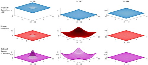
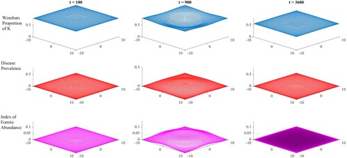
Figure 3. Spatiotemporal dynamics of scaled wombat abundance (as a proportion of the environmental carrying capacity, K – top row), the prevalence of mange in the wombat population (middle row), and the index of fomite abundance (represents the proportion of the theoretical maximum amount of fomites – lower row) when mite survival in the environment is low (7 days, ${\mu }_F=\frac{1}{7}$).

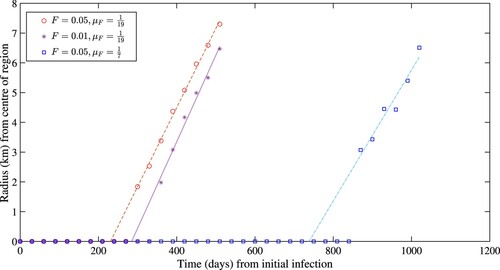
We additionally present an analysis of the speed over which mange disease spreads through space by measuring the distance between the centre of our modelled area from the peak of mange prevalence at 30-day intervals (Figure 4). The rate of mange spread is assessed under three conditions: standard number of mites and high environmental survival (F = 0.05, ${\mu }_F=\frac{1}{19}$); low number of mites and high environmental survival (F = 0.01, ${\mu }_F=\frac{1}{19}$); and standard number of mites and low environmental survival (F = 0.05, ${\mu }_F=\frac{1}{7}$).

Figure 4. A comparison between the speed of the wavefronts. The circles and asterisks are for a mite survival rate of 19 days (${\mu }_F=\frac{1}{19}$). The circles refer to a case where the height of the initial spike for fomites (F) was 0.05 and the asterisks refer to a case where the height was 0.01. Finally, the squares refer to the case of the mites having a lifespan off the host of 7 days (${\mu }_F=\frac{1}{7}$), and an initial spike height of 0.05.

5.1. Spatial patterns

Under high mite survival, we found that a travelling wave of mange disease was observed, as seen in Figure 2. The host population size was reduced across large areas of the modelled region by day 900; with wombats primarily persisting around the edges and corners, but the population rebounded to approximately one-third of the original population by day 3600, by which time it settled into a static spatial pattern. The survival of wombats in the corners of this domain is caused in part by the fact that the travelling wave of the disease reaches the edges at a later time. In addition, boundary conditions (6(6) $\frac{\mathrm{\partial }N}{\mathrm{\partial }x}=0$(6) ) and (7(7) $\frac{\mathrm{\partial }N}{\mathrm{\partial }y}=0$(7) ) influence wombat numbers significantly on the edges and in the corners, and different assumptions about wombat behaviour in these zones could lead to a different outcome. Intuitively fomite abundance tracked the disease prevalence to day 900; however, the fomite did not survive the host population bottleneck and became functionally extinct by day 3600. Under lower mite survival conditions, similar spatial dynamics were observed in Figure 3, although host population decline was much weaker, with the final population size roughly two-thirds of the original by day 3600. Again fomites became functionally extinct by day 3600 and the model moved to a static spatial pattern.

5.2. Spatial variation affecting long term survivability

The inclusion of spatial dynamics in a system that had previously only been modelled temporally [6, 7] resulted in significant outcome differences. We found under conditions of this model that the host population persisted even for a high fomite survival rate, as seen in Figure 2. Relative to a comparable aspatial model of mange in wombats, our results indicate that including spatial variation led to localized host extinction, but not global. Hosts appear subsequently able to recolonize mite-free regions, to support host population survival. While the host population was ultimately able to survive locally and then globally by day 3600, fomite extinction evidently occurred globally in both scenarios.

5.3. Travelling wave speed

A previous case study found an average speed of 338.3 m per year or 0.927 m per day spread of a travelling front of mange through a bare nosed wombat population, with the wave slowing down as it moved through the region [26]. Under the conditions of this model, the peak of the disease prevalence began moving outward in a travelling wave-like pattern from approximately day 300 (As seen in Figure 4). The radius of the peak of the disease prevalence from the centre of the region followed a linear relation from days 300 to 540, giving a constant wave speed that was calculated from a linear best fit to be 26.6 m per day from day 300. This measurement was repeated for a lower initial spike of fomite abundance, where the radius of the peak of the disease prevalence from the centre of the region followed a linear relation from days 360 to 510. A linear best fit for this second system was calculated and gave a wave speed of 29.1 m per day from day 360. These measurements were contrasted against a system with a lower mite life expectancy off the host, where the peak of the disease prevalence followed a linear relation from days 870 to 1020. A linear best fit for this was calculated and gave a wave speed of 22.2 m per day beginning from day 870. Each of these results plots, along with the linear best fit line, can be seen in Figure 4.

6. Discussion

The manner in which pathogens spread through an environment influences their spatial dynamic [18], but many models of dynamics are aspatial [32]. Here, we sought to characterize the spatial dynamics of environmentally transmitted S. scabiei among a wombat host population, a system that has not been previously modelled spatially. We created a system of partial differential equations to model the host-pathogen interaction, which we used to assess spatial variation in the survivability of wombats and characterize spatial behaviour of the system. We also calculated the rates of pathogen spread. We found that the inclusion of spatial variation led to population persistence in cases where aspatial models predicted extinction [6]. We found that sarcoptic mange moved through the host population as a travelling wave. We also observed that under the parameters considered, the wave speed was constant. Overall, this study supports the empirical observation of disease spread [26] and demonstrates the importance of including spatial factors in understanding disease dynamics.

While many disease dynamic models are aspatial, empirical disease spread is, of course, a spatial and temporal process. We found that the inclusion of spatial variability led to appreciable changes in host outcomes from mange disease. In both of our differing mite death rate scenarios, the wombat population persisted even though other research predicted extirpation from the lower mite death rate scenario [6, 7]. This research supports other studies, empirical and theoretical, showing how the inclusion of spatial variability can support population persistence [28], including research on metapopulation dynamics. This research also helps understand differing disease dynamics observed in wombats.

Past and emerging research suggests mange disease can be endemic [12, 25] with stable host populations of wombats [12], can cause epizootics that drive significant host decline [26] and the parasite can go locally extinct after introduction into a region [25, 26]. Our PDE system reinforces these dynamics, showing that these types of dynamics can be driven, in our case, by simply varying the environmental death rate of the mite laboratory studies have shown S. scabiei mites can survive up to 19 days under optimal environmental conditions (${10}^{\circ }$C, $95\mathrm{\%}$ RH). Recent field studies have estimated it may vary between 6 and 16 days [10], suggesting the ${\mu }_F$ values explored here are representative. Future empirical research following the long-term spatial and temporal dynamics of wombat populations will be valuable for further refining our understanding of disease dynamics in this system, and systems containing other similarly transmitted parasites.

Pathogens can spread through populations in many forms; for example, a range of research has reported forms such as spatially homogeneous dynamics at small spatial scales [31], oscillations that may persist [23] or dampen over time (with dampening leading to stable equilibrium states) [16] and travelling waves [26], among other forms [38]. Our modelling identified a travelling wave pattern of spread for mange disease prevalence in wombats; this pattern is supported by recent empirical research [26], which showed a travelling wave of mange disease prevalence driving wombat population decline in northern Tasmania. Our modelling estimate of wave speed (22.2 –29.1 m per day) was greater than the empirical estimate for wombats (0.9 m per day [26]), but similar to rates of mange spread estimated in other species (Vulpes vulpes, 10–30 m per day [36], Rupicapra rupicapra, 6–15 m per day [33]). This suggests that some parameters in our models may need further research, such as the spatial diffusion rate (σ) or transmission rate (β) [39], to ensure that the wave speed in our model matches better with those seen in nature. Interestingly, the northern Tasmania study population also appeared to have a relatively stable equilibrium of host population and disease prevalence prior to the epizootic event, and this likely indicates the importance of temporal variation in host and parasite life history and population parameters on disease dynamics (e.g. mite survival, host density, etc.). While beyond the scope of this study, research into seasonal and multi-annual changes in host and parasite life history and population parameters would be of value.

We adopted a set of parameters in our model that are, for the most part, based on empirical observations. Indeed, for wombats, a reasonable body of research exists to support the parameterization of models to characterize sarcoptic mange disease dynamics. Nevertheless, there are parameters that continue to be difficult to collect in the field and innovations in research would be of value to better understand this disease system. The rate at which wombats shed mites into their burrows and also their acquisition of mites within burrows is one example that remains poorly understood for logistical reasons. Similarly, while the home range movement of wombats is relatively well understood, aspects of dispersal are less well described. Finally, it is generally accepted that wombats can survive for approximately three months following infection with S. scabiei, but there is likely much variation around this estimate that is poorly understood and would benefit from investigations.

We sought to characterize the spatial dynamics of mange disease spread and S. scabiei among wombats, using a system of partial differential equations to model the host-pathogen interaction. We found that the inclusion of spatial variation led to population persistence in cases where aspatial models predicted extinction [6]. Sarcoptic mange was found to move through the host population as a travelling wave. We also observed that under the parameters considered, the wave speed was constant. Our research supports the empirical observation of disease spread [26] and demonstrates the importance of including spatial factors in understanding disease dynamics. This research may apply to the environmental transition of S. scabiei in other host species and potentially other similarly transmitted pathogens. Future research directions include, but are not limited to, considering a treatment model as part of this system, studying this system in the long term to track changing population states, considering re-introduction of disease in a long-term study, studies into temporally dependant changes to host and parasite life history, and population parameters and studying multiple differing host populations within a region.

Disclosure statement

No potential conflict of interest was reported by the author(s).

Additional information

Funding

This research was supported by an Australian Government Research Training Program Scholarship to IJH, and an Australian Research Council Linkage Project grant [LP180101251] to SC.

Appendix. Derivation of the linearized equations

In this section, we derive the system of linearized equations (8(8) $\begin{array}{rl}\frac{\mathrm{\partial }{S}_1}{\mathrm{\partial }t}& =\sigma {\mathrm{\nabla }}^2{S}_1+b{N}_1(1-2N_{\mathrm{eq}})-\mu S_1-\frac{\beta F_{\mathrm{eq}}{S}_1}{1+F_{\mathrm{eq}}}+\frac{\beta S_{\mathrm{eq}}{F}_1}{(1+F_{\mathrm{eq}}{)}^2},\end{array}$(8) )–(11(11) $\begin{array}{rl}\frac{\mathrm{\partial }{F}_1}{\mathrm{\partial }t}& =f(E_1+I_1)-{\mu }_F{F}_1.\end{array}$(11) ) by approximating full nonlinear system (1(1) $\begin{array}{rl}\frac{\mathrm{\partial }S}{\mathrm{\partial }t}& =\sigma {\mathrm{\nabla }}^{2}S+bN(1-N)-\frac{\beta SF}{1+F}-\mu S,\end{array}$(1) )–(4(4) $\begin{array}{rl}\frac{\mathrm{\partial }F}{\mathrm{\partial }t}& =f(I_L+I_H)-{\mu }_{F}F.\end{array}$(4) ) near an equilibrium $(S_{\mathrm{eq}},I_{L\mathrm{eq}},I_{H\mathrm{eq}},F_{\mathrm{eq}})$ at which the sub-populations of the wombats and the fomite populations have reached steady state.

Each population is expanded in a Taylor series, in some small parameter ε, about its equilibrium value. Mathematically, this is expressed by means of the equations (A1) $\begin{array}{rl}S& =S_{\mathrm{eq}}+\epsilon S_1+\mathcal{O}({\epsilon }^2),\\ I_L& =I_{L\mathrm{eq}}+\epsilon I_{L1}+\mathcal{O}({\epsilon }^2),\\ I_H& =I_{H\mathrm{eq}}+\epsilon I_{H1}+\mathcal{O}({\epsilon }^2),\\ F& =F_{\mathrm{eq}}+\epsilon F_1+\mathcal{O}({\epsilon }^2).\end{array}$(A1) The dimensionless number ε can be thought of as a measure of how much the system is perturbed away from its equilibrium state. The notation $\mathcal{O}({\epsilon }^2)$ refers to smaller terms of order ${\epsilon }^2$ and higher powers of ε.

These expressions (A1(A1) $\begin{array}{rl}S& =S_{\mathrm{eq}}+\epsilon S_1+\mathcal{O}({\epsilon }^2),\\ I_L& =I_{L\mathrm{eq}}+\epsilon I_{L1}+\mathcal{O}({\epsilon }^2),\\ I_H& =I_{H\mathrm{eq}}+\epsilon I_{H1}+\mathcal{O}({\epsilon }^2),\\ F& =F_{\mathrm{eq}}+\epsilon F_1+\mathcal{O}({\epsilon }^2).\end{array}$(A1) ) are now substituted into full nonlinear equations (1(1) $\begin{array}{rl}\frac{\mathrm{\partial }S}{\mathrm{\partial }t}& =\sigma {\mathrm{\nabla }}^{2}S+bN(1-N)-\frac{\beta SF}{1+F}-\mu S,\end{array}$(1) )–(4(4) $\begin{array}{rl}\frac{\mathrm{\partial }F}{\mathrm{\partial }t}& =f(I_L+I_H)-{\mu }_{F}F.\end{array}$(4) ). Taylor-series expansions in the parameter ε are also used to cope with the two nonlinear terms in original system (1(1) $\begin{array}{rl}\frac{\mathrm{\partial }S}{\mathrm{\partial }t}& =\sigma {\mathrm{\nabla }}^{2}S+bN(1-N)-\frac{\beta SF}{1+F}-\mu S,\end{array}$(1) )–(4(4) $\begin{array}{rl}\frac{\mathrm{\partial }F}{\mathrm{\partial }t}& =f(I_L+I_H)-{\mu }_{F}F.\end{array}$(4) ). The first of these two terms is $N(1-N)=N_{\mathrm{eq}}(1-N_{\mathrm{eq}})+\epsilon N_1(1-2N_{\mathrm{eq}})+\mathcal{O}({\epsilon }^2),$where N denotes the total wombat population $N=S+I_L+I_H$, as in Section 2. The second of the nonlinear terms in the full system is ${\displaystyle \frac{SF}{1+F}}={\displaystyle \frac{S_{\mathrm{eq}}{F}_{\mathrm{eq}}}{1+F_{\mathrm{eq}}}}+{\displaystyle \frac{\epsilon }{1+F_{\mathrm{eq}}}}[F_1{\displaystyle \frac{S_{\mathrm{eq}}}{1+F_{\mathrm{eq}}}}+S_1{F}_{\mathrm{eq}}]+\mathcal{O}({\epsilon }^2).$These approximations to the two nonlinear terms are substituted in system (1(1) $\begin{array}{rl}\frac{\mathrm{\partial }S}{\mathrm{\partial }t}& =\sigma {\mathrm{\nabla }}^{2}S+bN(1-N)-\frac{\beta SF}{1+F}-\mu S,\end{array}$(1) )–(4(4) $\begin{array}{rl}\frac{\mathrm{\partial }F}{\mathrm{\partial }t}& =f(I_L+I_H)-{\mu }_{F}F.\end{array}$(4) ), and terms at each order of the parameter ε are collected.

The zeroth-order terms (involving ${\epsilon }^0$) are simply the equilibrium populations, and these cancel since they are already (steady-state) solutions to the nonlinear equations. The terms of the first order in ε give the linearized approximation to full system (1(1) $\begin{array}{rl}\frac{\mathrm{\partial }S}{\mathrm{\partial }t}& =\sigma {\mathrm{\nabla }}^{2}S+bN(1-N)-\frac{\beta SF}{1+F}-\mu S,\end{array}$(1) )–(4(4) $\begin{array}{rl}\frac{\mathrm{\partial }F}{\mathrm{\partial }t}& =f(I_L+I_H)-{\mu }_{F}F.\end{array}$(4) ) near the equilibrium value. When collected together, they give Equations (8(8) $\begin{array}{rl}\frac{\mathrm{\partial }{S}_1}{\mathrm{\partial }t}& =\sigma {\mathrm{\nabla }}^2{S}_1+b{N}_1(1-2N_{\mathrm{eq}})-\mu S_1-\frac{\beta F_{\mathrm{eq}}{S}_1}{1+F_{\mathrm{eq}}}+\frac{\beta S_{\mathrm{eq}}{F}_1}{(1+F_{\mathrm{eq}}{)}^2},\end{array}$(8) )–(11(11) $\begin{array}{rl}\frac{\mathrm{\partial }{F}_1}{\mathrm{\partial }t}& =f(E_1+I_1)-{\mu }_F{F}_1.\end{array}$(11) ) in the text.

References

- R.M. Anderson and R.M. May, Infectious Diseases of Humans, OUP Oxford, Oxford, 1992.
- L.G. Arlian and M.S. Morgan, A review of Sarcoptes scabiei: Past, present and future, Parasit. Vectors 10(1) (2017), p. 297.
- L.G. Arlian, R.A. Runyan, S. Achar, and S.A. Estes, Survival and infectivity of sarcoptes scabiei var. canis and var. hominis, J. Am. Acad. Dermatol. 11(2) (1984), pp. 210–215.
- F. Astorga, S. Carver, E.S. Almberg, G.R. Sousa, K. Wingfield, K.D. Niedringhaus, P. Van Wick, L. Rossi, Y. Xie, P. Cross, S. Angelone, C. Gortázar, and L.E. Escobar, International meeting on sarcoptic mange in wildlife, June 2018, Blacksburg, Virginia, USA, Parasit. Vectors 11(1) (2018), p. 449.
- S.C. Banks, L.F. Skerratt, and A.C. Taylor, Female dispersal and relatedness structure in common wombats (vombatus ursinus), J. Zool. 256(3) (2002), pp. 389–399.
- N.J. Beeton, S. Carver, and L.K. Forbes, A model for the treatment of environmentally transmitted sarcoptic mange in bare-nosed wombats (vombatus ursinus), J. Theor. Biol. 462 (2019), pp. 466–474.
- N.J. Beeton, L.K. Forbes, and S. Carver, Comparing modes of transmission for sarcoptic mange dynamics and management in bare-nosed wombats, Lett. Biomath. 8(1) (2021), p. 318.
- S. Blumberg and J.O. Lloyd-Smith, Inference of R0 and transmission heterogeneity from the size distribution of stuttering chains, PLoS Comput. Biol. 9(5) (2013), p. e1002993.
- B.M. Bolker, A. Kleczkowski, and B.T. Grenfell, Seasonality and extinction in chaotic metapopulations, Proc. R. Soc. Lond. B: Biol. Sci. 259(1354) (1995), pp. 97–103.
- E. Browne, M.M. Driessen, R. Ross, M. Roach, and S. Carver, Environmental suitability of bare-nosed wombat burrows for sarcoptes scabiei, Int. J. Parasitol. Parasites Wildl. 16 (2021), pp. 37–47.
- A.A. Cunningham, P. Daszak, and J.L.N. Wood, One health, emerging infectious diseases and wildlife: Two decades of progress? Philos. Trans. R. Soc. B: Biol. Sci. 372(1725) (2017), p. 20160167.
- M.M. Driessen, E. Dewar, S. Carver, and R. Gales, Conservation status of common wombats in Tasmania. I: Incidence of mange and its significance, Pac. Conserv. Biol. 28(2) (2022), pp. 103–114.
- E.A. Eskew and B.D. Todd, Parallels in amphibian and bat declines from pathogenic fungi, Emerging Infect. Dis. 19(3) (2013), pp. 379–385.
- T.A. Fraser, M. Charleston, A. Martin, A. Polkinghorne, and S. Carver, The emergence of sarcoptic mange in Australian wildlife: An unresolved debate, Parasit. Vectors 9(1) (2016), p. 316.
- W.F. Frick, S.J. Puechmaille, and C.K.R. Willis, White-nose syndrome in bats, in Bats in the Anthropocene: Conservation of Bats in a Changing World, C.C. Voigt and T. Kingston, ed., Springer International Publishing, New York, 2015. pp. 245–262.
- G. Guzzetta, V. Tagliapietra, S.E. Perkins, H.C. Hauffe, P. Poletti, S. Merler, and A. Rizzoli, Population dynamics of wild rodents induce stochastic fadeouts of a zoonotic pathogen, J. Anim. Ecol.86(3) (2017), pp. 451–459.
- P.R. Hosseini, A.A. Dhondt, and A.P. Dobson, Spatial spread of an emerging infectious disease: Conjunctivitis in house finches, Ecology 87(12) (2006), pp. 3037–3046.
- P. Hudson, The Ecology of Wildlife Diseases, Oxford University Press, New York, 2002.
- A. Källén, P. Arcuri, and J.D. Murray, A simple model for the spatial spread and control of rabies, J. Theor. Biol. 116(3) (1985), pp. 377–393.
- C. Karimkhani, D.V. Colombara, A.M. Drucker, S.A. Norton, R. Hay, D. Engelman, A. Steer, M.Whitfeld, M. Naghavi, and R.P. Dellavalle, The global burden of scabies: A cross-sectional analysis from the global burden of disease study 2015, Lancet Infect. Dis. 17(12) (2017), pp. 1247–1254.
- M.J. Keeling and P. Rohani, Estimating spatial coupling in epidemiological systems: A mechanistic approach, Ecol. Lett. 5(1) (2002), pp. 20–29.
- W.O. Kermack and A.G. McKendrick, A contribution to the mathematical theory of epidemics, Proc. R. Soc. Lond. A 115(772) (1927), pp. 700–721.
- J. Lourenço and M. Recker, Natural, persistent oscillations in a spatial multi-strain disease system with application to dengue, PLoS Comput. Biol. 9(10) (2013), p. e1003308.
- A. Lunelli, An SEI model for sarcoptic mange among chamois, J. Biol. Dyn. 4(2) (2009), pp. 140–157.
- R.W. Martin, K.A. Handasyde, and L.F. Skerratt, Current distribution of sarcoptic mange in wombats, Aust. Vet. J. 76(6) (1998), pp. 411–414.
- A.M. Martin, C.P. Burridge, J. Ingram, T.A. Fraser, and S. Carver, Invasive pathogen drives host population collapse: Effects of a travelling wave of sarcoptic mange on bare-nosed wombats, J. Appl. Ecol. 55(1) (2018), pp. 331–341.
- A.M. Martin, S.A. Richards, T.A. Fraser, A. Polkinghorne, C.P. Burridge, and S. Carver, Population-scale treatment informs solutions for control of environmentally transmitted wildlife disease, J. Appl. Ecol. 56(10) (2019), pp. 2363–2375.
- T. Mononen and L. Ruokolainen, Spatial disease dynamics of free-living pathogens under pathogen predation, Sci. Rep. 7(1) (2017), p. 7729.
- J.V. Noble, Geographic and temporal development of plagues, Nature 250(5469) (1974), pp. 726–729.
- D.B. Pence and E. Ueckermann, Sarcoptic mange in wildlife, Rev. Sci. Tech. 21(2) (2002), pp. 385–398.
- I. Phillips, Ecology of infectious diseases in natural populations, B.T. Grenfell and A.P. Dobson, eds., University Press, Cambridge, 1995, Clin. Microbiol. Infect. 4(9) (1998), p. 536.
- M. Robinson, N.I. Stilianakis, and Y. Drossinos, Spatial dynamics of airborne infectious diseases, J. Theor. Biol. 297 (2012), pp. 116–126.
- L. Rossi, C. Fraquelli, U. Vesco, R. Permunian, G.M. Sommavilla, G. Carmignola, R. Da Pozzo, and P.G. Meneguz, Descriptive epidemiology of a scabies epidemic in chamois in the Dolomite Alps, Italy, Eur. J. Wildl. Res. 53(2) (2007), pp. 131–141.
- L.F. Skerratt, Clinical response of captive common wombats (vombatus ursinus) infected with sarcoptes scabiei var. wombati, J. Wildl. Dis. 39(1) (2003), pp. 179–192.
- L.F. Skerratt, R.W. Martin, and K.A. Handasyde, Sarcoptic mange in wombats, Aust. Vet. J. 76(6) (1998), pp. 408–410.
- C.D. Soulsbury, G. Iossa, P.J. Baker, N.C. Cole, S.M. Funk, and S. Harris, The impact of sarcoptic mange sarcoptes scabiei on the British Fox vulpes vulpes population, Mol. Ecol.15(14) (2007), pp. i–xviii.
- E.A. Stanley, D.L. Brown, and J.D. Murray, On the spatial spread of rabies among foxes, Proc. R. Soc. Lond. B., Biol. Sci. 229(1255) (1986), pp. 111–150.
- S.T. Stoddard, B.M. Forshey, A.C. Morrison, V.A. Paz-Soldan, G.M. Vazquez-Prokopec, H. Astete, R.C. Reiner, S. Vilcarromero, J.P. Elder, E.S. Halsey, T.J. Kochel, U. Kitron, and T.W. Scott, House-to-house human movement drives dengue virus transmission, Proc. Natl. Acad. Sci. 110(3) (2012), pp. 994–999.
- J. Tamura, J. Ingram, A.M. Martin, C.P. Burridge, and S. Carver, Contrasting population manipulations reveal resource competition between two large marsupials: Bare-nosed wombats and eastern grey kangaroos, Oecologia 197(2) (2021), pp. 313–325.
- D.M. Tompkins, S. Carver, M.E. Jones, M. Krkosek, and L.F. Skerratt, Emerging infectious diseases of wildlife: A critical perspective, Trends Parasitol. 31(4) (2015), pp. 149–159.
- B. Triggs, Wombats, 2nd ed., CSIRO Publishing, Collingwood VIC, 2009.
- P. Van Rooij, A. Martel, F. Haesebrouck, and F. Pasmans, Amphibian chytridiomycosis: A review with focus on fungus-host interactions, Vet. Res. 46(1) (2015), p. 137.
- L.A. White, J.D. Forester, and M.E. Craft, Dynamic, spatial models of parasite transmission in wildlife: Their structure, applications and remaining challenges, J. Anim. Ecol. 87(3) (2017), pp. 559–580.
- World Health Organisation. Scabies. (2017). https://www.who.int/news-room/fact-sheets/detail/scabies.