Comparison of classical tumour growth models for patient derived and cell-line derived xenografts using the nonlinear mixed-effects framework

Abstract

In this study we compare seven mathematical models of tumour growth using nonlinear mixed-effects which allows for a simultaneous fitting of multiple data and an estimation of both mean behaviour and variability. This is performed for two large datasets, a patient-derived xenograft (PDX) dataset consisting of 220 PDXs spanning six different tumour types and a cell-line derived xenograft (CDX) dataset consisting of 25 cell lines spanning eight tumour types. Comparison of the models is performed by means of visual predictive checks (VPCs) as well as the Akaike Information Criterion (AIC). Additionally, we fit the models to 500 bootstrap samples drawn from the datasets to expand the comparison of the models under dataset perturbations and understand the growth kinetics that are best fitted by each model. Through qualitative and quantitative metrics the best models are identified the effectiveness and practicality of simpler models is highlighted

Keywords:

• Cancer
• mixed-effects
• mathematical modelling

1. Introduction

In the process of preclinical evaluation of drug effects on tumours, an essential first step is the accurate modelling of tumour kinetics and the appropriate choice of tumour growth model to do so. Inferring which mathematical model is the best to describe tumour growth kinetics is performed through comparing the fit of the model to the data which is very often done in the context of fitting each model to single growth curves individually. Previous studies have focused on comparing tumour models in that manner over the past decades [3,4,16,24], with few focusing on a plethora of mathematical models including empirical, functional and structural tumour models. The results from such studies are comparable with a few exceptions owning to different fitting optimization methods and variance assumptions [4,17]. More specifically, in [17] with the exception of the logistic and von Bertalanffy model which were unable to describe the data, the other 12 models captured the dynamics sufficiently with the Gompertz model being one of the best performing empirical models and superior to the exponential particularly in the case of spheroid dynamics. Similarly in [4] the Gompertz model is at the top two performing models in both the breast cancer data along with the exponential-linear model, which is the Simeoni model used in our study, as well as the lung data together with the power law model. The paper by Benzekry et al. [4] is very interesting due to the fact that the comparison of the model is performed using both individual fits and mixed-effects with data from 20 mice for lung cancer and 34 mice for breast cancer (2 cell lines) and several goodness-of-fit metrics were used.

Fitting of models to individual curves might limit our understanding of which model is best at capturing a given dataset as a whole and at simulating xenograft growth in general. That has led to the use of nonlinear mixed-effects, which allow for a simultaneous fit of the model to the totality of the data, being the most popular approach for pharmacokinetics/pharmacodynamics (PK/PD) analysis in the pharmaceutical industry. Nonlinear mixed-effects (NLME) models are statistical models that allow for both fixed-effects that stay constant at every measurement and random-effects that change depending on the sample/level (individuals) [20]. As a result they can account for different types and levels of variability in addition to residual errors and hence give rise to multilevel/hierarchical structures. Due to the ability of NLME models to capture correlations between data, such as multiple measurements from the same study or from the same individual, they are very suitable for modelling multiple tumour growth data since they can fit the whole dataset without the need to fit each curve individually or assume independence [6] and hence lead to more generalized results. Rarely are NLME models used for large preclinical datasets with the work by Parra-Guillen et al. [22] being the first large dataset systematic modelling of xenografts using that framework and the paper by Benzekry et al. [4] being the only model comparison paper using mixed-effects. To the best of our knowledge our paper is the first that performs a model comparison in such extensive datasets for both patient-derived xenografts (PDXs) and cell-line derived xenografts (CDXs) and attempting to generalize by comparing the performance of tumour growth models under perturbations of the original dataset.

This paper is focused on xenograft data and more particularly patient-derived and cell-derived ones. These come from either direct engraftment of tumour tissue from the patient to immuno-deficient mice (PDX) or by in vitro cultivation of the tumour cell-lines that are then engrafted to immuno-deficient mice (CDX). Xenografts have advantages over the classic cell-line studies as they are considered to be more heterogeneous and their micro-environment more similar to that of the patient tumour [27]. That has led to xenograft studies becoming very popular for cancer research as they are deemed a more appropriate model for comparison to clinical studies. Among these, PDXs are considered an even better approximation due to the fact that CDX have already been exposed to an artificial culture environment perhaps leading to loss of their characteristics [27]. On the other hand, the direct tissue engraftment of PDX preserves both the original micro-environment and cell–cell interactions [15].

2. Materials and methods

2.1. Data

In this project we explore the performance of seven mathematical models, extensively used in the context of tumour growth, by fitting them on PDX data from the Novartis PDX encyclopedia found in the supplementary material of Gao et al. [12] and internal AstraZeneca CDX data.

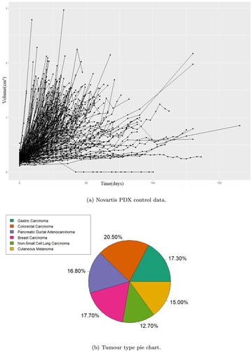
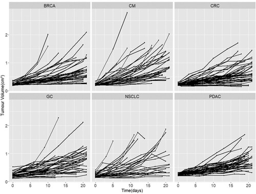
Data used for the comparison of the mathematical models came from pre-existing studies, no animal experiments were performed for the current study. The data come from two different sources the first being the Novartis PDX encyclopedia which is the biggest publicly available database of PDX data. As the primary aim of this study is the fitting of the models on pure growth we considered only the untreated (control) cases which comprise of 220 volume change data from 220 PDXs without replicates (no. of 1) with six different tumour types, namely breast carcinoma (BRCA), non-small cell lung carcinoma (NSCLC), gastric cancer (GC), colorectal cancer (CRC), cutaneous melanoma (CM) and pancreatic ductal carcinoma (PDAC) as shown in Figure 1. There were 2442 datapoints in total. The authors Gao et al. [12] showed the effect of the genetic drift due to passages was minimal with the PDXs demonstrating phenotypic stability and PDX from the same patient having almost perfect expression correlation. To make sure the drift was minimized the study in Gao et al. was conducted with PDXs between 4 and 10 passages.

Figure 1. The control data from the Novartis patient derived xenograft (PDX) studies in their totality and the distribution of PDX per cancer type in that dataset. The PDX control data demonstrate large variability in growth rates and on average slower growth than the CDX data. (a) Novartis PDX control data. (b) Tumour type pie chart.

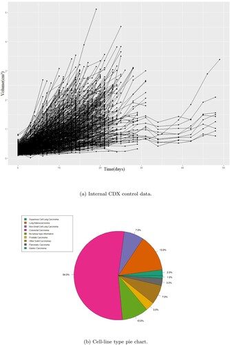
The second source was internal CDX studies. All animals studies in the United Kingdom were conducted in accordance with the UK Home Office legislation, the Animal Scientific Procedures Act 1986, and with AstraZeneca Global Bioethics Policy. For PD studies, tumour cells were subcutaneously inoculated into athymic nude mice and measured in regular intervals (initially several times a week) using calipers. These data originate from independent studies. Mice were sacrificed when the total tumour weight reach the specified welfare limit (2.5 $c{m}^3$). There were 25 cell lines in total (with multiple replicates in each) that spans several different tumours. Data as well as tumour distribution per cell-line can be seen in Figure 2.

Figure 2. The control data from the internal cell-line derived xenograft (CDX) studies in their totality and the distribution of CDXs per cancer type in that dataset including replicates. The CDX control data show more uniform dynamics and faster on average growth rates compared to the PDX data. (a) Internal CDX control data. (b) Cell-line type pie chart.

The range of measurements varied widely for individual mice with the longest measurement being at 165 days for the Novartis dataset and 45 for the internal. Due to the different growth rates, we observe something called a dropout where fast-growing cancers are terminated early which biases the fitting towards calculating a slower average growth rate [13]. Hence, there is the need to introduce a cut-off at the measurements, one that is long enough so that we have enough data points but short enough as to minimize the effect of the dropout and keep as many mice as possible. Figure 3 shows a comparison of the different cut-off times for the Novartis data.

Figure 3. Potential cut-off points with a step of 10 and 20 days, respectively. The number next to the vertical lines indicate the number of mice left above that threshold. (a) Cut-offs with 10 days step. (b) Cut-offs with 20 days step.

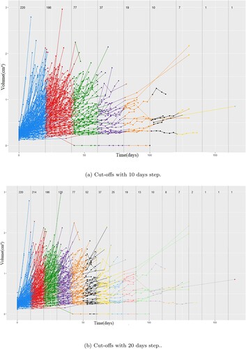
We want to keep the framework for the comparison as similar as possible between studies and hence we introduce the same cut-off to the CDX dataset as well. A similar analysis for that dataset is not required as the cut-off does not decrease the number of samples.

We can see that mice are being taken off the study at every possible cut-off but perhaps the most dramatic change is the difference in growth curves from the cut-off of 20 to 30 days with 186 animals being left after 20 but 120 after 30. This can also be seen when the step is 20 days. That indicates that a cut-off of around 20 days is both a reasonable time-frame for the curves to have evolves as well as a point where still the majority of models remain with a good representation of both fast and slow growing tumours. Although an exploration of the optimal number around the 20th day mark was not performed we selected 21 days to represent exactly three weeks of measurements decreasing the dataset to 1359 datapoints.

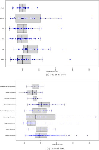
We did not find strong evidence to suggest that different tumour types demonstrate different growth kinetics (see Figure 4) and hence we aggregated the data from all tumour types together for the fitting and comparison of the models.

Figure 4. Boxplot and beeswarm of growth rates for individual patient derived xenografts and cell-line derived xenografts curves fitting using the exponential model in MATLAB. The cancer type abbreviations are breast carcinoma (BRCA), non-small cell lung carcinoma (NSCLC), gastric cancer (GC), colorectal cancer (CRC), cutaneous melanoma (CM) and pancreatic ductal carcinoma (PDAC). (a) Gao et al. data. (b) Internal data.

2.2. Tumour growth models

Various mathematical models have been formulated to capture tumour growth each with different assumptions and simplifications. We focus on five models which have been widely used for this purpose.

2.2.1. Exponential model

(1) $\frac{\mathrm{d}V}{\mathrm{d}t}=k_{e}V.$(1) The exponential model is the simplest of models used for that purpose. It assumes that a tumour is growing proportionally to its volume at a constant rate given by the growth parameter k, leading to an unbounded growth. Although that is the case in early stages of tumour growth [5] evidence suggests a slowing down of the initial rate [21] and after a certain size for various reasons, one being the inability of oxygen reaching the inner part of the tumour resulting in a hypoxic centre that does not contribute to the overall growth. That translates in the growth law changing to something different than an exponential for larger tumours.

2.2.2. Gompertz model

(2) $\frac{\mathrm{d}V}{\mathrm{d}t}=aV-bVln(V).$(2) The Gompertz model was formulated in 1825 by Benjamin Gompertz and has since found many applications in biology where the curves take a S-shape form. In tumour dynamics in particular the equation accounts for the progressive decrease of the growth rate as the tumour gets larger. For small volumes the first term dominates and the growth law is almost exponential. Whereas for higher values it slows down significantly leading to a steady-state for V. Two possible explanations have been given the for the second term in the Gompertz model one being a possible aging$/$differentiation of cells which increases the doubling time of cells and the other being the diffusion limited dynamics of oxygen on the inside of the tumour assuming a critical concentration below which hypoxia occurs giving rise to a hypoxic radius [7]. The disadvantage of this method is the fact that a steady-state has not been observed experimentally.

2.2.3. Simeoni model

(3) $\begin{array}{rl}\frac{\mathrm{d}V}{\mathrm{d}t}& ={\lambda }_{0}V,V\le V_{th},\end{array}$(3) (4) $\begin{array}{rl}\frac{\mathrm{d}V}{\mathrm{d}t}& ={\lambda }_1,V>V_{th}.\end{array}$(4) Which, are often combined in one equation: (5) $\frac{\mathrm{d}V}{\mathrm{d}t}=\frac{{\lambda }_{0}V}{{[1+{\left(\frac{{\lambda }_0}{{\lambda }_1}V\right)}^{\psi }]}^{1/\psi }}.$(5) The exponential-linear model which for simplicity we will call the Simeoni model [23] is built around a similar idea to the Gompertz model where tumour growth starts as exponential and switches to linear with the difference that the volume does not reach a steady-state but instead keeps growing at steady rate after the switch. The critical volume at which this happens can be expressed in terms of the two growth parameters in order to have continuity ($V_{th}={\lambda }_1/{\lambda }_0$). The parameter ψ was kept fixed at the value 20 as in the original paper in order to not introduce a third parameter into the model. This corresponds to the switching parameter and a high enough value, as tested in [23], offers a smooth and rapid switching comparable to the two-equation system.

2.2.4. Conger model

(6) $\begin{array}{rl}\frac{\mathrm{d}V}{\mathrm{d}t}& =K_{c}V(1-{(1-\frac{r_d}{r})}^3),r>r_d\end{array}$(6) (7) $\begin{array}{rl}\frac{\mathrm{d}V}{\mathrm{d}t}& =K_{c}V.\end{array}$(7) This model first appeared in the paper by Conger and Ziskin [8] following the observation that tumour spheroids went from a geometric to a linear growth with a constant proliferating shell radius and it was later formulated to account for drug effects [10]. It is based on the hypoxic core idea for limiting growth rate, where the growth rate is multiplied by the proliferating fraction, i.e. the outer layer of the cell tumour that contributes to the proliferation. The parameter $r_d$ is the difference of the total radius of the tumour and of the hypoxic core radius and is considered to be constant and specific to each cancer type. As the tumour increases the proliferating fraction becomes smaller and for very high values approximating only the surface of the tumour. The growth rate although decreasing never becomes zero and hence the model admits no steady-state. r is the radius of the whole tumour given by $(\pi 3/4V{)}^{1/3}$.

2.2.5. Mayneord model

(8) $\frac{\mathrm{d}V}{\mathrm{d}t}=K_m{V}^{2/3}.$(8) In 1932 W. V. Mayneord [18] formulated a model to describe Jensen's rat sarcoma re-derived and adjusted to account for PD effects [14]. The basic assumption of this model is that the rate of growth of the radius of the tumour is constant which gives rise to the equation above for the volume. It can be shown, using asymptotic analysis for large tumour volumes, that this model represents a special case of the Conger model and the growth is mainly originating from the surface of the tumour, hence the 2/3 exponent.

2.2.6. Logistic model

(9) $\frac{\mathrm{d}V}{\mathrm{d}t}=aV(1-\frac{V}{K}).$(9) The Logistic model was formulated by Pierre Francois Verhulst [25]. Similar to the Gompertz model it assumes a slowing down of the growth rate that is linear with respect to the increasing volume of the tumour. The model assumes a carrying capacity for the tumour volume that when reached makes the growth rate go to zero.

2.2.7. von Bertanlanffy

(10) $\frac{\mathrm{d}V}{\mathrm{d}t}=a{V}^{\gamma }-bV.$(10) The von Bertanlanffy model [26] was derived based on the idea that growth is a balance between metabolic and catabolic processes. The model assumes that the former often follows an allometric scaling whereas the latter is proportional to the total volume. While often the model appears with $\gamma =2/3$ we wanted to include the more general form for the comparison.

2.3. Fitting and comparison

A nonlinear mixed-effects model was fitted to the data, which allows for a more complete capturing of the data by taking into account all individual data, inter-individual variability, dependence of measurements and ignoring missing values. In NLME the parameters of the model are made up of two components that are estimated in this setting. Fixed-effects which represent the average dynamical behaviour and average value of the parameter (population value) and random-effects which represent the variability of the parameters between individuals in the population. Mixed-effects can be summarized with the following equations: $\begin{array}{rl}{y}_{ij}& =f(p_i,x_{ij})+{ϵ}_{ij}\\ p_i& =A_i\theta +B_i{\eta }_i\\ {\eta }_i& \sim N(0,{\omega }^2)\\ {ϵ}_{ij}& \sim N(0,{\sigma }^2)\end{array}$Where, $y_{ij}$ is the response j for individual i, $p_i$ is parameter i given by the sum of fixed-effects ${\theta }_i$ and random-effects ${\eta }_i$, $A_i,B_i$ are design matrices for fixed and random-effects and ${ϵ}_i$ are residuals errors. Both the residual errors and the random-effects are assumed to be normally distributed with mean zero and variance ${\sigma }^2$ and ${\omega }^2$, respectively. Hence, in contrast to typical model fitting NLME calculates a distribution for each parameter centred around θ with variance ${\omega }^2$.

This was done in the programming environment R using the NLMIXR package v1.1.0.9 [11] with proportional error and no covariance between different parameters and the FOCEi method in order to account for the interaction between the known and unknown variability [2]. Log-likelihood for the FOCEi method can be found in [2] Equations (10(10) $\frac{\mathrm{d}V}{\mathrm{d}t}=a{V}^{\gamma }-bV.$(10) )–(11(11) $AIC=2k-ln(\mathcal{L}).$(11) )) and depends on both residual errors as well as inter-individual variability. The initial tumour volume was fitted as a parameter. Moreover, the covariance matrix is fully diagonal assuming that there were no correlations between the parameters. This was done for the sake of simplicity and any strong correlation would manifest itself in the diagnostic plots if present as an inadequacy of the model to fit the data.

Before fitting the models using the nonlinear mixed-effects framework we needed to provide initial estimates for the initial conditions, parameters as well as their between subject variability. To do that we performed individual curve fittings with an additive least squares error (lsqcurvefit) in the programming language MATLAB. That gave us estimates of the mean parameter values as well as their variance. Additionally it showed that the different tumours have similar growth characteristics for these PDXs as seen in Figure 4. A similar conclusion was draw for the CDXs especially since half of the data (with replicates treated separately) are from CRC.

The performance of the NLME fitting was assessed using both goodness-of-fit criteria namely VPCs in order to assess the ability of the model to fit the actual data and the degree of over or under-prediction as well as the quantitative metric of Akaike Information Criterion number to compare the performance of the models between one another [1]. AIC number is derived from information theory and the smaller it is the better is the performance of the model. It penalizes overfitting by introducing a positive parameter number term and rewards the quality of the fitting. The equation is given by: (11) $AIC=2k-ln(\mathcal{L}).$(11) Where k is the number of parameters for a given model and $\mathcal{L}$ is the likelihood.

Since we wanted to generalize our results beyond our datasets it was not enough to derive the AIC number for the fitting of the models to our dataset. There is no statistic or distribution associated with the AIC that allows a p-value to be generated in order to assign significance to the differences in AIC scores. To that end we performed the fitting of the models to 500 bootstrap samples of the original datasets with resampling [9]. The reason for that is that each bootstrap sample is a perturbation of the original dataset hence the comparison of the model in all 500 perturbation is a form of sensitivity analysis on the model comparison, i.e. a way of seeing how changes to the initial dataset affect the results with the hope that a model will outperform the other in all or most samples. Moreover, the 500 simulations provide 500 AICs for each model which give rise to AIC distributions. Additionally, using visual interpretations of the individual objective functions for each model for each growth curve we aimed to explain the characteristics that favour one model compared to another.

Finally, for the case of the Novartis PDX dataset, where we have an almost even distribution of the data among 6 tumour types, we fitted the models to each type individually to access whether the optimal model is tumour type dependent and how the models perform on a study-like dataset size. For that purpose we used the AIC directly.

3. Results

Tables 1 and 2 show the fitted values of the model parameters for the Gao et al. and internal dataset, respectively. The initial estimate for the starting tumour volume was 0.24 for all models in the PDX dataset and 0.4 for all models in the CDX. The parenthesis next to the estimated value contains the relative standard error as a percentage and the one next to the BSV contains the coefficient of variation (CV). The initial tumour volume, V(0), was fitted as a parameter and attained very similar estimate and variability in all models which is to be expected.

Table 1. Model parameters, fitting errors and AIC for Gao et al. PDX dataset.

Model	Parameter	Definition	Initial estimate	Final estimate (RSE%)	BSV(CV%)	Error(ϵ)	AIC
Exponential	K	Growth rate(1/day)	0.1	0.051(1.4%)	66.7	0.123	−2838
Gompertz	a	Growth rate(1/day)	0.05	0.036(1.8%)	101	0.111	−2999
	b	Limiting growth coefficient(1/day)	0.02	0.016(2.3%)	215
Simeoni	${\lambda }_0$	Exponential growth rate(1/day)	0.1	0.054(3.6%)	81.9	0.114	−2936
	${\lambda }_1$	Linear growth rate($c{m}^3/day$)	0.2	0.087(6.5%)	57.9
Conger	K	Growth rate(1/day)	0.4	0.67(30%)	55.2	0.119	−2931
	$r_d$	Proliferating shell thickness(cm)	0.007	0.012(2.8%)	56
Mayneord	K	Growth rate(cm/day)	0.4	0.038(1.5%)	83.3	0.119	−2935
Logistic	a	Growth rate(1/day)	0.2	0.067(1.9%)	84.6	0.113	−2974
	K	Carrying capacity($c{m}^3$)	2.1	2.04(11.4%)	55
von Bertanlanffy	a	Anabolic rate($c{m}^{3(1-\gamma )}/day$)	0.9	0.88(3.05%)	37.3	0.111	−2997
	b	Catabolic rate(1/day)	0.05	0.047(4.4%)	14
	γ	Allometric scaling(-)	0.66	0.98(10.6%)	187

Notes: This table holds the initial estimates and final estimated parameter values for each model fitted to the original Gao et al. [12] dataset including the between subject variability and precision of estimation. Additionally we provide the goodness-of-fit criteria including the error and AIC number.

Table 2. Model parameters, fitting errors and AIC for internal CDX dataset.

Model	Parameter	Definition	Initial estimate	Final estimate (RSE%)	BSV (CV%)	Error(ϵ)	AIC
Exponential	K	Growth rate(1/day)	0.1	0.09(0.6%)	36.6	0.166	−4466
Gompertz	a	Growth rate(1/day)	0.1	0.076(0.8%)	54.4	0.137	−5431
	b	Limiting growth coefficient(1/day)	0.4	0.037(1.4%)	132
Simeoni	${\lambda }_0$	Exponential growth rate(1/day)	0.1	0.11(0.2%)	64.9	0.139	−5304
	${\lambda }_1$	Linear growth rate($c{m}^3/day$)	0.4	0.11(0.4%)	56.5
Conger	K	Growth rate(1/day)	0.6	0.97(60%)	39.9	0.153	−5030
	$r_d$	Proliferating shell thickness(cm)	0.02	0.018(15%)	24.7
Mayneord	K	Growth rate(cm/day)	0.2	0.078(0.7%)	47.7	0.153	−5038
Logistic	a	Growth rate(1/day)	0.2	0.134(1.13%)	50.8	0.139	−5436
	K	Carrying capacity($c{m}^3$)	2.6	2.47(3.9%)	42.2
von Bertanlanffy	a	Anabolic rate($c{m}^{3(1-\gamma )}/day$)	0.9	0.147(2.21%)	25.8	0.137	−5412
	b	Catabolic rate(1/day)	0.05	0.069(3.1%)	11.5
	γ	Allometric scaling(-)	0.66	0.96(6.1%)	187

Notes: This table holds the initial estimates and final estimated parameter values for each model fitted to the original internal. dataset including the between subject variability and precision of estimation. Additionally we provide the goodness-of-fit criteria including the error and AIC number.

From the fitting of the PDX dataset (AIC & error) we observe that the Gompertz and von Bertanlanffy models seem to provide the best fit followed by the Logistic and then the Simeoni, Mayneord and Conger that have similar AIC numbers and finally the exponential which as expected is the worst performing. This can also be seen from the proportional error in the model with the Gompertz and von Bertnalnaffy having approximately $11.1\mathrm{\%}$ error. Interestingly the Gompertz model also demonstrates the greatest variability in its parameters between different PDXs as seen from the large BSV (random effect). In contrast the Conger model required the smallest variability in order to describe the data among all models. In the case of the Conger model we also see the larger estimation error for the growth parameter but that is attributed to the high correlation between the K and $r_d$ making it challenging to tell one apart from the other precisely.

In the fitting of the CDX dataset the Logistic model has the lowest AIC with the Gompertz and von Bertanlanffy models having slightly larger AIC values but with lower errors. In contrast to the PDX dataset the Simeoni model demonstrates a differential performance compared to the Conger and Mayneord which have both a higher AIC and a higher error. Despite the large number of individual curves of the CDX dataset we observe a decrease in the variability needed to describe the data from all models in addition to a significant increase in the growth rate. These differences are evident in Figures 1(a) and 2(a) of the growth curves.

Figure 5 and 6 are a comparison of the VPCs between the different models where the mean growth curves as well as the $95\mathrm{\%}$ prediction intervals are shown for each dataset, the complete VPCs with the 97.5 and 2.5 percentiles as well as the 95% confidence intervals are included as well in Figure 7 and 8. All of these were produced from 500 simulated datasets. Supplementary Figures S1–S6 demonstrate other goodness-of-fit plots and namely the observations vs IPRED, the residuals plot as well as the residuals versus observation. IPRED corresponds to the ‘individual prediction’ which is the simulation of the model using the fixed effects as well as the individual random effects, in contrast to PRED which corresponds to the ‘population prediction’, i.e. the simulation of the average model using only the fixed effects. These plots serve as further indication of the ability of a model to capture the data, satisfy the normality of residuals and make sure there is no underlying trend in the residuals with varying values of the volume. These are in agreement with the conclusion made so far regarding the ability of the modes to fit the data. The residuals are normal-like in all cases, no miss-specification pattern is observed in the weighted residual vs time or vs PRED plots. In the observation vs IPRED plots we notice that most models follows the data quite well with some over and under predictions for higher tumour sizes for certain models.

Figure 5. Comparison of mean curves and $95\mathrm{\%}$ prediction intervals for the five models fitted to Gao et al. dataset. Black dashed curve is the model mean curve.

Figure 6. Comparison of mean curves and $95\mathrm{\%}$ prediction intervals for the five models fitted to internal CDX dataset. Black dashed curve is the model mean curve.

Figure 7. Visual predictive checks (VPCs) for the seven models on the Gao et al. patient derived xenograft dataset. The black solid line represents the observation mean curve and the dotted the 97.5 and 2.5 percentiles for the observations, i.e the data. The thick dashed line is the simulated data mean. The three shaded blue areas are the 95% confidence intervals from the 500 simulated datasets of the model with the fitted parameter values for the model mean and the model 97.5 and 2.5 percentiles.

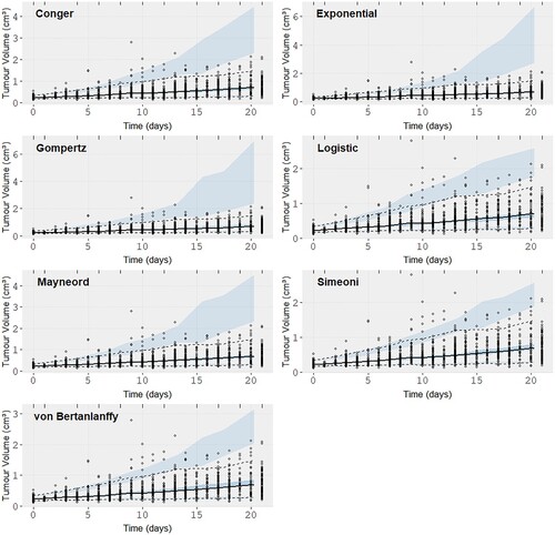
Figure 8. Visual predictive checks (VPCs) for the seven models on the internal cell-line derived xenografts. The black solid line represents the observation mean curve and the dotted the 97.5 and 2.5 percentiles for the observations, i.e the data. The thick dashed line is the simulated data mean. The three shaded blue areas are the 95% confidence intervals from the 500 simulated datasets of the model with the fitted parameter values for the model mean and the model 97.5 and 2.5 percentiles.

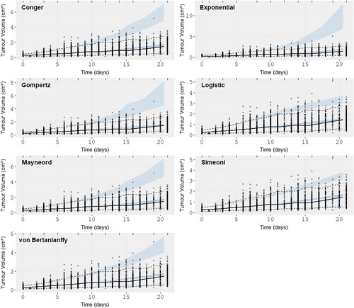
From the VPCs we are looking for prediction intervals that follow the data closely. Von Bertanlanffy and the Logistic model seem to offer the best fit (VPC) in both datasets with the Simeoni model showing a similar performance to them for the CDX dataset only. The exponential seems to over-predict the data variability and the other three models are almost indistinguishable. From the Observation vs IPRED plots (S1,S4) we can see the individual predictions from the Gompertz and von Bertanlannfy model capture the observations the best compared to other models which show no distinct difference between them other than in the higher volume regions where we can observe that the Gompertz and von Bertanlanffy are still true to the observations. The Simeoni and Logistic models predict lower volumes than the ones observed and the other three models predict higher volumes than the observations with the results of the Exponential being the worst. Finally the WRES vs Observation (S3,S6) plots are almost indistinguishable, mainly showing no trend which would indicate a miss-specification of the model, with the exception of negative residual trend observed for large volumes in the case of the CDX dataset for the Simeoni and Exponential model, and so are the residual plots. So while there were some differences in the different VPCs no clear picture can be painted regarding the best model and most seem to perform very adequately for both datasets. That raised the need for the use of a quantitative metric.

Moving from the VPCs to the AIC numbers from 500 bootstrap samples the comparison becomes clearer.

From Figure 9(a) and Table 3 we can see that the Gompertz and von Bertanlanffy models are the best performing models (AIC distribution) in the PDX dataset, outperforming all others. They are followed by the Logistic, Mayneord, Conger and Exponential in order of performance. In the case of the CDX dataset Figure 9(b) the Logistic model has the lowest AIC values distribution followed closely by the Gompertz and then the von Bertanlanffy. In contrast to the PDX dataset here the Simeoni model outperforms both Conger and Mayneord. This highlights the importance of comparing the models on multiple samples. If the results were drawn from the original dataset a comparison between the Simeoni, Mayneord and Conger would be impossible but the bootstrap analysis allows for more generalized picture of their performance and what we see instead is a clear distinction. The results are summarized in Tables 3 and 4 where we give the probability of model A in a column outperforming model B in a row as the number of bootstrap samples the model A had smaller AIC than model B divided by the total number of bootstrap samples (500). Supplementary Figures S7–S8 show the distributions AIC values for each model in the same axis.

Figure 9. Histograms of the difference between Akaike Information Criterion (AIC) numbers from the 500 bootstrap samples for each couple of models fitted to the Novartis and Internal datasets, respectively. (a) Gao et al. bootstrap samples histogram. (b) Internal bootstrap samples histogram.

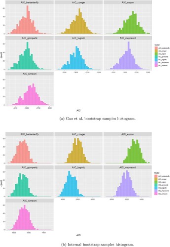
Table 3. Performance summary of models in the 500 bootstrap samples for PDX dataset.

	Conger	Exponential	Gompertz	Logistic	Mayneord	Simeoni	von Bertanlanffy
Conger	–	0.028	1	0.918	0.968	0.194	1
Exponential	0.972	–	1	0.92	1	0.974	1
Gompertz	0	0	–	0.014	0	0	0.466
Logistic	0.082	0.08	0.986	–	0.084	0.1	0.932
Mayneord	0.032	0	1	0.916	–	0.152	1
Simeoni	0.806	0.026	1	0.9	0.848	–	1
von Bertanlanffy	0	0	0.534	0.068	0	0	–

Note: This table holds the probability that a model in a column is better than a model in row for the patient-derived xenografts dataset based on the number of samples the first model had better AIC number than the second model divided by 500 which is the total number of bootstrap samples.

Table 4. Performance summary of models in the 500 bootstrap samples for CDX dataset.

	Conger	Exponential	Gompertz	Logistic	Mayneord	Simeoni	von Bertanlanffy
Conger	–	0	0.952	0.964	0.974	0.994	1
Exponential	1	–	0.994	0.998	1	0.994	1
Gompertz	0.048	0.006	–	0.594	0.048	0.068	0.318
Logistic	0.044	0.004	0.406	–	0.044	0.05	0.292
Mayneord	0.006	0	0.952	0.956	–	0.994	1
Simeoni	0.006	0.006	0.932	0.95	0.006	–	0.984
von Bertanlanffy	0	0	0.682	0.708	0	0.016	–

Note: This table holds the probability that a model in a row is better than a model in column for the cell-derived xenografts dataset based on the number of samples the first model had better AIC number than the second model divided by 500 which is the total number of bootstrap samples.

Most of the distributions seem normally distributed but we can observe a few outliers. That might be due to the fact that there were some odd growth curves in both datasets, i.e. tumour shrinkage, which growth models cannot account for.

Moving on to now try and understand why the models perform the way they do we have used the objective function value for the individual sample(unique ID) to see if there is a pattern that explains which models fits which dynamics better.

Figure 10 illuminates some of the reasons why certain models perform better. For example it is clear in the Novartis dataset that there were many slow growing tumours that are captured well by the Gompertz. The Exponential, Mayneord and Logistic seem to be good at fast growing tumours. The Simeoni is doing well across the whole board and finally the von Bertanlanffy captures the extremities well, i.e. the very fast and very slow growing tumours.

Figure 10. Growth curves coloured depending on which model had the best objective function value for each curve. Curves are in log scale for internal data and normal scale for Novartis dataset. (a) Gao et al. dataset. (b) Internal dataset.

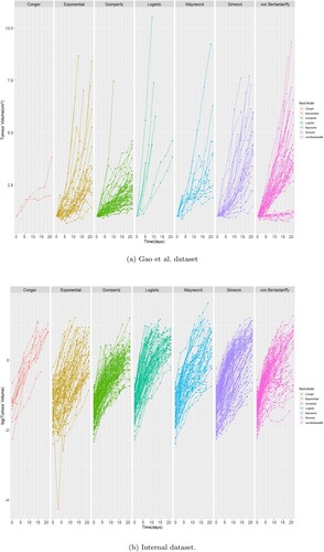
In the Internal dataset we used a log scale to make the results clearer. Here we observe the exponential model is fitting curves that are almost straight line as expected whereas the rest of the models do well for curves that differ from the typical straight line log-curve. There is also a significantly larger amount of curves fitted better by the Simeoni model. Other than that no additional information can be drawn from these plots.

Another interesting observation is the good performance of the Gompertz (as seen from Figure 10) despite not seeing the classical sigmoidal curves that it is so good at capturing. Possible explanations can be the fact that there is a significant number of slow-growing tumour that the Gompertz model is able to capture due to the flexibility and variability of the retardation term in Equation (2(2) $\frac{\mathrm{d}V}{\mathrm{d}t}=aV-bVln(V).$(2) ) and also the fact that the slowing down of the tumour is done continuously compared to the Simeoni model that features a switch or the Mayneord model that has the same form throughout.

As a final exploratory step into the performance of the models and wanted to check whether that is tumour and dataset-size dependent we fitted the models to each tumour type. That was performed only for the Novartis dataset as only there do we have an almost even split of curves per tumour type (internal dataset is CRC dominated).

Table 5 summarizes the results of the fitting on individual tumour types. The initial estimates are kept the same as the before. The shrinkage for each parameter of the model was added to aid in identifying potential issues. Shrinkage, defined as 1-SD(between individual variation)/Ω, approaches zero when data are informative and 1 otherwise with high shrinkage indicating an issue in estimating the inter-individual variation of the parameter. What is in agreement with the previous results is that the Gompertz model is once again consistently one of the top performers (AIC & error). It outperforms all the other models in 3 out of 6 tumour types and it is the second best in CRC and PDAC. Surprisingly it perform quite poorly in NSCLC. The von Bertanlanffy and Logistic models generally perform well but have variable performance and often high shrinkage indicating a difficulty in evaluating some parameters in the presence of fewer data. Another expected result is the exponential model being consistently one of the worst models similar to what we saw earlier.

Table 5. Summary of fitting each model to each tumour type separately.

	AIC	Position	Error	Value (RSE%)	BSV (CV%)	Shrink(SD)%
Exponential(BRCA)	−619	6	0.092	0.05(3.36%)	70.6%	3.35%
Simeoni(BRCA)	−615	7	0.093	0.05(3.34%) 0.28(8.62%)	70.6% 31.2%	3.25% 93.4%
Conger(BRCA)	−627	5	0.091	0.62(1110%) 0.01(126%)	44.4% 68.7%	44.6% 20.5%
Mayneord(BRCA)	−628	3	0.092	0.037(3.6%)	84.6%	2.62%
Gompertz(BRCA)	−634	1	0.086	0.04(4.6%) 0.01(5.1%)	106% 165%	12.3% 34.9%
Logistic(BRCA)	−628	2	0.084	0.068(20.6%) 2.09(50.2%)	79.2% 101%	1.62% 32.2%
von Bertanlanffy(BRCA)	−627	4	0.087	0.055(5.1%) 0.013(9.9%) 0.97(43%)	57.2% 43.9% 187%	8.31% 75.9% 46.6%
Exponential(CM)	−348	7	0.133	0.07(3.36%)	54.2%	2.8%
Simeoni(CM)	−423	2	0.102	0.09(4.1%) 0.1(4.2%)	90.3% 54.9%	9.12% 37.3%
Conger(CM)	−384	6	0.12	0.87(7180%) 0.01(236%)	61.2% 28.8%	11.4% 57.5%
Mayneord(CM)	−388	5	0.12	0.06(3.78%)	69.8%	1.71%
Gompertz(CM)	−428	1	0.098	0.06(4.24%) 0.02(6.78%)	79.1% 272%	9.02% 22.7%
Logistic(BRCA)	−421	4	0.098	0.068(20.6%) 2.09(50.2%)	79.2% 101%	1.62% 32.2%
von Bertanlanffy(BRCA)	−421	3	0.095	0.094(6.8%) 0.034(12.1%) 0.9(38.7%)	42.2% 76.8% 187%	22.1% 39.3% 13.7%
Exponential(CRC)	−668	7	0.115	0.04(2.97%)	70.9%	6.14%
Simeoni(CRC)	−721	4	0.101	0.05(3.97%) 0.05(2%)	92.2% 45.7%	3.34% 77.4%
Conger(CRC)	−697	6	0.108	0.6(153%) 0.01(17.8%)	61.5% 61.2%	31.8% 34%
Mayneord(CRC)	−702	5	0.108	0.03(3.36%)	93.8%	5.18%
Gompertz(CRC)	−728	2	0.098	0.03(4.51%) 0.02(4.77%)	130% 243%	21.9% 23.8%
Logistic(BRCA)	−724	3	0.099	0.062(5.42%) 1.42(47.9%)	107% 42.6%	4.86% 49%
von Bertanlanffy(BRCA)	−746	1	0.096	0.095(4.64%) 0.066(6.8%) 0.98(22.1%)	22.0% 26.3% 187%	29.8% 45.2% 28.9%
Exponential(GC)	−434	6	0.123	0.04(3.35%)	60.9%	9.03%
Simeoni(GC)	−431	7	0.123	0.04(3.12%) 0.19(23.1%)	62.6% 60.4%	9.35% 85.2%%
Conger(GC)	−444	5	0.117	0.61(260%) 0.01(29.1%)	49.3% 55.3%	36.9% 31.7%
Mayneord(GC)	−447	4	0.117	0.03(3.38%)	79.1%	7.82%
Gompertz(GC)	−459	1	0.109	0.03(4.03%) 0.02(5.46%)	96.7% 202%	21.2% 31.6%
Logistic(BRCA)	−450	3	0.112	0.065(5.13%) 1.69(39.6%)	80.3% 49.5%	7.64% 52.9%
von Bertanlanffy(BRCA)	−451	2	0.109	0.083(9.64%) 0.051(12.3%) 0.98(31.9%)	32.3% 10.2% 187%	11.8% 84.2% 40.2%
Exponential(NSCLC)	−247	3	0.167	0.06(5.43%)	94.3%	6.53%
Simeoni(NSCLC)	−246	4	0.167	0.06(4.94%) 0.15(10.1%)	99.4% 28.1%	8.37% 82.7%
Conger(NSCLC)	−248	2	0.166	0.23(21%) 0.06(14.4%)	9.44% 148%	84.8% 7.67%
Mayneord(NSCLC)	−249	1	0.167	0.04(5.63%)	118%	5.64%
Gompertz(NSCLC)	−244	5	0.165	0.05(6.12%) 0.01(9.34%)	115% 293%	9.77% 59.2%
Logistic(BRCA)	−247	3	0.167	0.073(6.19%) 2.79(16.6%)	108% 12.4%	6.4% 93.7%
von Bertanlanffy(BRCA)	−243	6	0.166	0.071(6.35%) 0.019(10.4%) 0.98(36.6%)	70.4% 30.3% 23.5%	3.33% 82.8% 93%
Exponential(PDAC)	−599	7	0.118	0.05(1.95%)	36.7%	6.54%
Simeoni(PDAC)	−603	6	0.116	0.05(2.1%) 0.08(1.23%)	40.2% 6.34%	6.64% 97.1%
Conger(PDAC)	−605	5	0.116	0.63(2380%) 0.01(254%)	31.9% 33.2%	33.6% 33%
Mayneord(PDAC)	−609	1	0.115	0.04(2.19%)	45.8%	4.16%
Gompertz(PDAC)	−607	2	0.114	0.03(3.01%) 0.02(4.52%)	53% 119%	19.3% 54.2%
Logistic(BRCA)	−606	4	0.116	0.061(3.04%) 2.26(18.9%)	45.3% 10.9%	5.34% 90.9%
von Bertanlanffy(BRCA)	−606	3	0.114	0.056(4.23%) 0.017(9.23%) 0.97(40.5%)	24.8% 45% 183%	25.1% 54.5% 45%

Note: The position, i.e. performance is decided by the AIC number and error in case of equal AIC values.

Despite some similarities with the results from before, there were a few note-worthy observations. The first is the Simeoni's model performance. While there were 2 tumours where it performs well (compared to other models) in the rest it seems to be at the last positions according to the AIC number. While the difference in performance is not clear from the dynamics observed in Figure 11 the very high shrinkage of the linear growth term might indicate a difficulty in evaluating that parameter. That is in agreement to [22] where the authors reported a difficulty in evaluating the BSV of the linear growth term as well as in addition to having the largest error compared to the other model parameters. That was not the case when all tumours were combined in a single large dataset. This in turn might indicate a potential issue with using this model in smaller datasets, normal study-size datasets were there were not enough data from the linear phase of the growth. This difficulty in evaluating parameters (high shrinkage) is also evident in the Logistic and von Bertanlanffy models which might suffer from similar estimation issues in smaller datasets.

Figure 11. Novartis PDX growth curves per tumour type. Growth curves of the PDXs from Novartis dataset stratified according to the tumour type. The cancer type abbreviations are breast carcinoma (BRCA), non-small cell lung carcinoma (NSCLC), gastric cancer (GC), colorectal cancer (CRC), cutaneous melanoma (CM) and pancreatic ductal carcinoma (PDAC).

The second observation is the performance of the Mayneord model which is the top performers in two cases without ever dropping below position 5. That is a surprising result taking into account that this is the only single parameter model that performs well and even outperforms more complicated models. That is somewhat in agreement to the our results from the fitting of the full dataset (AIC bootstrap) where the Mayneord's model performance was superior to that of the Conger and Simeoni.

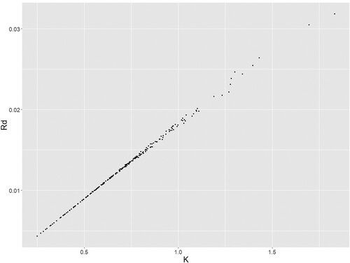
Additionally, we can see some very large error associated with the parameters of the Conger model and that stems from the strong correlation between them. That can be seen in Figure 12 from the NLME fitting of the Conger model to the PDX dataset. We can see a very strong trend between the two parameters. Additionally, in the tumour type specific fittings a strong correlation between the fitted values of $K_c$ and $r_d$ was observed even reaching a value of 1 making them indistinguishable. That is again an issue that needs to considered when dealing with the Conger model is smaller datasets.

Figure 12. Conger parameters values for individual fits. The parameter values of the Conger model using NLME to fit it to the PDX data.

Finally, it should be stressed that although our analysis was performed in the original data scale we fitted the models in the log-transformed data for both datasets which admitted the same results with respect to model comparison and similar errors and parameter estimates. For that reason we deemed that it would not strongly affect the subsequent analysis. Similarly the Baysian Information Criterion (BIC) was evaluated as an alternative measure instead of the AIC and yielded the same results and conclusions. Hence, we deemed it not necessary to include both AIC and BIC in the analysis.

4. Conclusions

In this paper we compared seven mathematical models for tumour growth using nonlinear mixed-effects on two large datasets. To our knowledge this is the first model comparison on this setting and with the use of different xenograft models. Both data and analysis highlight novelty compared to previous studies, namely the two large datasets of different xenografts in addition to the use of the bootstrap that generalizes the comparison for the seven models under dataset perturbations. Two datasets were used in order to assess the models in different situations as PDXs and CDXs might have different growth patterns. The models selected for this comparison are simple empirical models and one structural (Conger) with most of them admitting an initial exponential growth and a subsequent decrease in growth rate. The comparison of the models was performed both quantitatively and visually. Visual comparison and analysis was essential to confirm that all models are capable of capture the base dynamics of the data and the quantitative comparison using AIC on bootstrap samples was necessary to formalize and generalize the results.

The Gompertz model was consistently one of the best performing by all means of comparison that include the fitting of the models to the original datasets, the AIC bootstrap, the VPCs as well as the comparison in the fitting of each tumour type. This is in agreement to several studies of model fitting in both in vitro and in vivo data [4,17,19]. From the individual curves objective function value we were able to determine that the niche of the Gompertz model at the slower growing tumours. Despite the fact that the CDX data admit faster growing growth curves the Gompertz model remained one of the top performing models possibly due to the fact of the second term in the equation that allows for a continuous slowing down of the growth rate and hence a more flexible model. The analysis shows that this model is not only appropriate for sigmoidal dynamics but it also has the potential to capture varying tumour growths. The von Bertanlanffy and Logistic model also proved to be two of the best performing models with their performance being a bit more variable compared to the Gompertz and in the case of fewer data (fitting of individual tumour types) with difficulties in the estimation of some model parameters. The worst performing model is almost always the exponential model, with the exception of the fitting of some tumour types, which despite the fact that it captures the mean dynamics effectively, overpredicts the overall growth due to the lack of slowing down during at later time points. That was expected as it is the simpler model on which most of the other models are based. The other three models have variable performance depending on the dataset with the Mayneord model showing a comparable performance in the VPCs with more complicated models and even better performance with respect to the AIC distributions to two parameters models such as the Simeoni and Conger in the PDX dataset. Moreover, the Conger model parameter estimates have the smallest variability in the PDX dataset and one of the smallest in the CDX in contrast to the Gompertz that has the largest.

The distinction between the CDX and PDX data is understandable as the CDX growth curves are faster growing and more homogeneous as can be seen by the parameter estimates as well as the respective figures. That favours models such as the Simeoni whose transition from exponential to linear volume change is more suitable to faster dynamics compared to the Mayneord a model whose growth is sub-exponential from the beginning and linear in radial change. The small proliferating shell thickness found in the Conger model means that the majority of the tumours are fitted as if they have a necrotic core from the beginning and hence with a sub-exponential growth as well. The flexibility of the Simeoni model switching becomes evident in Figure 10(a) where it is clear that the model is able to capture the widest range of growth curves better than the other models, from almost stationary tumours to very fast growing ones.

It is worth mentioning that a comparison of the models using only the datasets is not comprehensive as the errors are comparable and the VPC are in most cases indistinguishable between models such as the Gompertz, Conger and Mayneord. The bootstrap analysis of the AIC is what provides evidence on the order of performance of the models. With both these results in mind it might be important to consider other factors when selecting a model for tumour growth. For example despite the differences found through AIC the Mayneord model, from the VPCs, seems to be performing well and similarly to the other models despite the fact that it has only one parameter compared to the two of Simeoni, Conger, Gompertz, Logistic and von Bertanlanffy which might become important when extending the model to treated tumours which will result in more parameters added. This is highlighted even further when comparing the models by fitting them to each tumour type separately. That allows for a comparison in a more realistic scale similar to what you would have in an tumour study.

With regards to the fitting on individual tumour types no conclusions can be drawn as to which model is better at capturing a specific type without additional datasets to explore and no such conclusion was clear from the dynamics of the curves themselves. The AIC numbers in many cases were comparable and the positioning of the models is not there to state categorically which model is statistically better but mainly as an additional point to the aforementioned argument that considerations other than strict statistical performance might be important when deciding which model to select for further analysis.

Moving on from the comparison of these models, potential future work could include comparing even more models including other empirical ones as well as complex mechanistic models to have a fuller picture of the performance of tumour models on PDX and CDX data. An other potential future direction of this work is a similar analysis but by fitting the model on a log scale with a additive error. That would allow to explore any difference in the analysis and results obtained by using different fitting approaches. Additionally in the log scale the growth curves will be compressed on a tighter range which might lead to model niches different from the ones observed in Figure 9. Whether that would lead to a better insight of the performance of these models is uncertain but different assumptions on the data fitting process have shown different preferences in models in some occasions [17].

Acknowledgments

We thank Matthew Fidler for his help and advice on modelling and fitting in NLMIXR.

Disclosure statement

D.V. and K.C.B. are full-time employees and shareholders of AstraZeneca. DV was a PostDoc fellow of the AstraZeneca PostDoc programme. J.W.T.Y. was an employees of AstraZeneca.

Additional information

Funding

Funded by AstraZeneca. Dimitrios Voulgarelis is a fellow of the AstraZeneca Postdoc Programme.

References

- H. Akaike, On entropy maximization principle, Appl. Stat. (1977), pp. 27–41.
- J. Almquist, J. Leander, and M. Jirstrand, Using sensitivity equations for computing gradients of the foce and focei approximations to the population likelihood, J. Pharmacokinet. Pharmacodyn. 42 (2015), pp. 191–209.
- Ž. Bajzer, S. Vuk-Pavlović, and M. Huzak, Mathematical Modeling of Tumor Growth Kinetics, A Survey of Models for Tumor-Immune System Dynamics, Springer, 1997, pp. 89–133.
- S. Benzekry, C. Lamont, A. Beheshti, A. Tracz, J.M. Ebos, L. Hlatky, and P. Hahnfeldt, Classical mathematical models for description and prediction of experimental tumor growth, PLoS. Comput. Biol. 10 (2014), p. e1003800.
- M. Bissery, P. Vrignaud, F. Lavelle, and G. Chabot, Experimental antitumor activity and pharmacokinetics of the camptothecin analog irinotecan (cpt-11) in mice., Anticancer. Drugs. 7 (1996), pp. 437–460.
- H. Brown and R. Prescott, Applied Mixed Models in Medicine, John Wiley & Sons, Edinburgh, 2014.
- A.C. Burton, Rate of growth of solid tumours as a problem of diffusion, Growth 30 (1966), pp. 157–176.
- A.D. Conger and M.C. Ziskin, Growth of mammalian multicellular tumor spheroids, Cancer Res. 43 (1983), pp. 556–560.
- B. Efron, Estimating the error rate of a prediction rule: Improvement on cross-validation, J. Amer. Statist. Assoc. 78 (1983), pp. 316–331.
- N.D. Evans, R.J. Dimelow, and J.W. Yates, Modelling of tumour growth and cytotoxic effect of docetaxel in xenografts, Comput. Methods Programs. Biomed. 114 (2014), pp. e3–e13.
- M. Fidler, J.J. Wilkins, R. Hooijmaijers, T.M. Post, R. Schoemaker, M.N. Trame, Y. Xiong, and W.Wang, Nonlinear mixed-effects model development and simulation using nlmixr and related r open source packages, CPT: pharmacometrics Syst. Pharmacol. 8 (2019), pp. 621–633.
- H. Gao, J.M. Korn, S. Ferretti, J.E. Monahan, Y. Wang, M. Singh, C. Zhang, C. Schnell, G. Yang, Y.Zhang, and O.A. Balbin, High-throughput screening using patient-derived tumor xenografts to predict clinical trial drug response, Nat. Med. 21 (2015), pp. 1318–1325.
- J.W. Hogan and N.M. Laird, Model-based approaches to analysing incomplete longitudinal and failure time data, Stat. Med. 16 (1997), pp. 259–272.
- N.L. Jumbe, Y. Xin, D.D. Leipold, L. Crocker, D. Dugger, E. Mai, M.X. Sliwkowski, P.J. Fielder, and J. Tibbitts, Modeling the efficacy of trastuzumab-dm1, an antibody drug conjugate, in mice, J. Pharmacokinet. Pharmacodyn. 37 (2010), pp. 221–242.
- J. Jung, H.S. Seol, and S. Chang, The generation and application of patient-derived xenograft model for cancer research, Cancer Res. Treat.: Official J. Korean Cancer Assoc. 50 (2018), pp. 1–10.
- M. Marušić, Ž. Bajzer, J. Freyer, and S. Vuk-Pavlović, Analysis of growth of multicellular tumour spheroids by mathematical models, Cell. Prolif. 27 (1994), pp. 73–94.
- M. Marušić, S. Vuk-Pavlovic, and J.P. Freyer, Tumor growth in vivo and as multicellular spheroids compared by mathematical models, Bull. Math. Biol. 56 (1994), pp. 617–631.
- W.V. Mayneord, On a law of growth of Jensen's rat sarcoma, Am. J. Cancer. 16 (1932), pp. 841–846.
- S. Michelson, A. Glicksman, and J. Leith, Growth in solid heterogeneous human colon adenocarcinomas: Comparison of simple logistical models, Cell. Prolif. 20 (1987), pp. 343–355.
- D. Mould and R.N. Upton, Basic concepts in population modeling, simulation, and model-based drug development part 2: Introduction to pharmacokinetic modeling methods, CPT: Pharmacometrics Syst. Pharmacol. 2 (2013), pp. 1–14.
- L. Norton and R. Simon, Growth curve of an experimental solid tumor following radiotherapy, J. Natl. Cancer Inst. 58 (1977), pp. 1735–1741.
- Z.P. Parra-Guillen, V. Mangas-Sanjuan, M. Garcia-Cremades, I.F. Troconiz, G. Mo, C. Pitou, P.W.Iversen, and J.E. Wallin, Systematic modeling and design evaluation of unperturbed tumor dynamics in xenografts, J. Pharmacol. Exp. Ther. 366 (2018), pp. 96–104.
- M. Simeoni, P. Magni, C. Cammia, G. De Nicolao, V. Croci, E. Pesenti, M. Germani, I. Poggesi, and M. Rocchetti, Predictive pharmacokinetic-pharmacodynamic modeling of tumor growth kinetics in xenograft models after administration of anticancer agents, Cancer Res. 64 (2004), pp. 1094–1101.
- V.G. Vaidya and F.J. Alexandro Jr, Evaluation of some mathematical models for tumor growth, Int. J. Biomed. Comput. 13 (1982), pp. 19–35.
- P.F. Verhulst, Notice sur la loi que la population suit dans son accroissement, Corresp. Math. Phys.10 (1838), pp. 113–126.
- L. Von Bertalanffy, Problems of organic growth, Nature 163 (1949), pp. 156–158.
- E. Yada, S. Wada, S. Yoshida, and T. Sasada, Use of Patient-Derived Xenograft Mouse Models in Cancer Research and Treatment, 2017.