
 ?Mathematical formulae have been encoded as MathML and are displayed in this HTML version using MathJax in order to improve their display. Uncheck the box to turn MathJax off. This feature requires Javascript. Click on a formula to zoom.
Abstract
A mathematical model with the intraguild predation structure is proposed to describe the interactions of autotrophs and mixotrophs containing light and nutrients in a well-mixed aquatic ecosystem. The dissipation, existence and stability of equilibria of the model are proved, and the ecological reproductive indexes for the extinction, survival and coexistence of autotrophs and mixotrophs are established. We also consider the influence of Holling type functional responses and abiotic factors on the coexistence and biomass of autotrophs and mixotrophs. It is shown that the intraguild predation structure is beneficial to phytoplankton biodiversity and provides an explanation for the phytoplankton paradox.
1. Introduction
Algae, as typical phytoplankton, are the primary producer of organic compounds in the whole aquatic ecosystem. They form the basis of energy flow and material circulation in lakes or oceans. Algae mainly consist of two parts: autotrophs (autotrophic algae) and mixotrophs (mixotrophic algae). Autotrophs synthesize organic matters through photosynthesis to supply their own growth [Citation1, Citation11, Citation17, Citation18]. Mixotrophs as the combination of autotrophic and heterotrophic nutrition not only use photosynthesis to combine inorganic matters into organic matters, but also feed on microorganisms to meet their growth [Citation2, Citation3].
The interaction of autotrophs and mixotrophs is complicated containing competition and predation (see Figure ). The growth of autotrophs is affected by nutrition and light [Citation1, Citation10, Citation23, Citation29]. There is no obvious dichotomy for mixotrophs as producers or consumers. In general, autotrophic activities and heterotrophic activities of mixotrophs are carried out at the same time. In the autotrophic situation, the metabolism of mixotrophs is also limited by light and nutrients. This indicates that in this case, autotrophs and mixotrophs compete for light [Citation2, Citation14] or nutrients [Citation15, Citation16, Citation24, Citation25]. Mixotrophs in the heterotrophic nutrition can ingest micro-autotrophs [Citation14, Citation24, Citation25].
Figure 1. The interactions between autotrophs and mixotrophs.
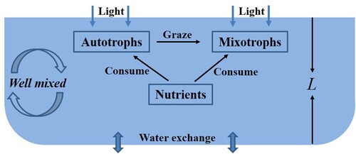
Intraguild predation is a ubiquitous ecological phenomenon in natural ecosystems [Citation5, Citation20]. It describes a relationship in which the predator not only consumes the prey, but also shares the same resource with the prey. From the relationship between autotrophs and mixotrophs, they form an intraguild predation structure. Previous studies have shown that autotrophs and mixotrophs compete only for nutrients [Citation15, Citation16, Citation24, Citation25] or only for light [Citation14]. Light comes from the water surface and gradually weakens with the depth of the water [Citation4, Citation19, Citation23]. Nutrients come from the bottom of the lake, and spread to the whole lake with the turbulence [Citation6, Citation27, Citation28]. Due to the importance of nutrients and light on the metabolism of autotrophs and mixotrophs [Citation1, Citation23, Citation29], it is essential to investigate the intraguild predation structure between autotrophs and mixotrophs with nutrients and light.
According to the above considerations and the existing research results, we propose and analyse a mathematical model of autotroph–mixotroph interactions with the intraguild predation structure. Our model contains the effect of light and nutrients. Through the analysis of the model, we investigate the dynamical behaviours for the survival, extinction and coexistence of autotrophs and mixotrophs, and consider Holling type functional responses, light and nutrients on the coexistence of autotrophs and mixotrophs. Here, we also try to study the ‘Paradox of the Plankton’ based on the model. This paradox, proposed by Hutchinson [Citation9], generally describes that the diversity of phytoplankton deviates from the limitation of the available abiotic resources in the same ecological niche.
Algal blooms are a natural ecological phenomenon of algae mass-breeding in the water source. It seriously affects aquatic ecological communities, water quality, and even threatens people's health. Algal blooms are caused by many reasons, including biotic and abiotic factors [Citation1, Citation27, Citation29]. The motivation of this paper is to explore the effect of biotic and abiotic factors on the blooms of autotrophic algae and mixotrophic algae. Based on our model, we will consider the biomass density of autotrophs and mixotrophs with the change of some important environmental parameters.
We construct this paper as follows. In Section 2, a dynamical model describing the interaction of autotrophs and mixotrophs is established in the intraguild predation structure. Then, we study dynamical features of this model containing dissipation of the solutions, the existence and stability of non-negative stable solutions in Section 3. In Section 4, by using some numerical simulations, we investigate the effect of abiotic and biotic factors on the coexistence and density of autotrophs and mixotrophs at a steady state with biologically reasonable parameters, and it explains their effects in phytoplankton biodiversity and blooms. Section 5 summarizes our results and proposes some research prospects to be studied in the future.
2. The model
We establish a dynamical model with the intraguild predation structure to describe the interactions of autotrophs and mixotrophs containing light and nutrients. Here, we consider a well-mixed aquatic environment such as a water column [Citation7, Citation8, Citation14] or epilimnion in lakes [Citation23, Citation29]. Let z represent the water depth coordinate. Then z = 0 denotes the water surface, and z = L denotes the bottom of the water column or epilimnion. Our model consists of three ordinary differential equations and one algebraic equation, characterizing the rate of change for autotrophs (A), mixotrophs (M) and dissolved nutrients (N) and light intensity (). Table lists the information on variables and parameters of the model.
Table 1. The variables and parameters of model (Equation3(3)
(3) ).
Light from the water surface is absorbed by the water body and phytoplankton. The light intensity at depth z can be described by the Lambert–Beer law [Citation7] as
The growth of autotrophs or mixotrophs in the autotrophic situation are limited by the light intensity
and dissolved nutrients N. It takes the form of multiplication of the two [Citation8, Citation23, Citation29] and is expressed as
Here, we assume that
satisfy
(1)
(1) Typical expressions for
and
are Monod functions [Citation8, Citation23]:
(2)
(2) In the heterotrophic condition, mixotrophs supply their own growth by ingesting autotrophic organisms [Citation14, Citation24, Citation25]. The predation rate of mixotrophs to autotrophs is
, where
is assumed to satisfy
Based on the principle of ecological stoichiometry [Citation11], the conversion rate satisfies
.
The reduction of biomass of autotrophs and mixotrophs mainly contains lost biomass due to death and respiration, sinking biomass
and water exchange biomass
[Citation23]. In addition, the predation of mixotrophs will also lead to the decline of autotrophic biomass.
The change of dissolved nutrients N consists of three parts. The first part depends on consumption by autotrophs and mixotrophs with a consumption rate
The second part is nutrient recycling from the loss of autotrophic and mixotrophic with recycling proportion
and the nutrients to carbon quota
. The last part is nutrient exchange
at the bottom of the water column or epilimnion, where
is a fixed nutrient input concentration.
According to the above discussion, we have the following autotroph–mixotroph interaction model in a well-mixed aquatic environment:
(3)
(3) Considering the biological significance of (Equation3
(3)
(3) ), we assume that all the parameters in Table are positive and
. By using rigorous mathematical arguments, we can draw the conclusion that for any positive initial value, (Equation3
(3)
(3) ) admits a unique positive solution defined for all
.
3. Qualitative analysis
In this section, we explore the dynamics of (Equation3(3)
(3) ) containing dissipation of the solutions, the existence and stability of non-negative steady-state solutions. The following theorem concludes the positive invariance and dissipation of the solutions of model (Equation3
(3)
(3) ).
Theorem 3.1
The system (Equation3(3)
(3) ) is dissipative.
Proof.
Let , which is the total nutrients in system (Equation3
(3)
(3) ). A direct calculation gives
This implies that
and the system (Equation3
(3)
(3) ) is dissipative.
Let
It follows from Theorem 3.1 that Δ is a global attracting region of system (Equation3
(3)
(3) ) and positively invariant.
3.1. Semi-trivial steady states
It follows from (Equation3(3)
(3) ) that the possible non-negative semi-trivial steady states are listed below:
Nutrient-only semi-trivial steady state
.
Nutrient-autotroph semi-trivial steady state
Nutrient-mixotroph semi-trivial steady state
We define the following ecological reproductive indexes for autotrophs and mixotrophs:
and
As an indicator of viability for autotrophs or mixotrophs,
, i = 0, 1, describe the average number of new autotrophs (mixotrophs) produced by one cubic metre of autotrophs (mixotrophs) in a life cycle of autotrophs (mixotrophs). In the following discussion, it is shown that
and
, i = 0, 1 are four critical values for autotrophs and mixotrophs to invade aquatic ecosystems, respectively.
The following result shows that (Equation3(3)
(3) ) always has a unique nutrient-only semi-trivial steady state
, which is also stable in terms of the ecological reproductive index
.
Theorem 3.2
always exists and it is globally asymptotically stable if
, while
is unstable if
.
Proof.
It is clear that always exists. The Jacobian matrix at
is
where
If
, then real parts of all the eigenvalues of the characteristic equation of
are negative. This implies that
is locally asymptotically stable. On the contrary, if
, then
is unstable.
It follows from Theorem 3.1 that . From (Equation3
(3)
(3) ), we have
for sufficiently large t. This means that
if
. The second Equation of (Equation3
(3)
(3) ) becomes
By the comparison theorem,
if
. By using the theory of asymptotical autonomous systems [Citation13], model (Equation3
(3)
(3) ) can reduce to a limiting system
This implies that
and
is globally attractive. Then
is globally asymptotically stable.
Remark 3.1
is a critical value for algae to survive in a well-mixed aquatic environment. It is affected by the nutrient input concentration
and the water surface light intensity
. It can be observed directly that
is increasing with respect to
and
. This means that the high light intensity and nutrient input concentration are conducive to the invasion of algae.
Theorem 3.3
If
Proof.
From (Equation4(4)
(4) ), we have
Note that
is strictly monotone decreasing with respect to A with
It follows from (Equation1
(1)
(1) ) that
is strictly monotone increasing with respect to A with
Then there exists a unique positive
such that
if and only if
. From the first equality of (Equation4
(4)
(4) ),
can be explicitly solved.
The Jacobian matrix at is
where
From (Equation1
(1)
(1) ), we have
A direct calculation gives
If
, then
. To conclude, we have
This shows that the real parts of all the eigenvalues of the characteristic equation of
are negative. Hence we conclude that if
, then
is locally asymptotically stable; Conversely, if
, then
is unstable.
Remark 3.2
The conclusion in Theorem 3.3 reveals that is a critical value for autotrophs from extinction to survival. If
, then autotrophs win the competition in the intraguild predation and dominate the whole aquatic ecosystem. This implies that
is a threshold value for mixotrophs to survive in the water ecosystem in the presence of autotrophs.
Theorem 3.4
If
Proof.
The proof of (i) has many similarities with Theorem 3.3. Then, we omit the proof process here. The Jacobian matrix at is
where
Similar to the proof of Theorem 3.3, we prove that the real parts of eigenvalues of
are all negative if
, which means that
is locally asymptotically stable. On the contrary,
is unstable if
.
Remark 3.3
Theorem 3.4 shows that exists if
and
is the index of threshold determining the survival of mixotrophs. Here, we only obtain the local stability of
. Actually, our numerical simulations indicate that
should be globally asymptotically stable. This means that if
, then mixotrophs win the competition in the intraguild predation structure. Autotrophs invade successfully only when
.
3.2. Coexistence steady states
This subsection is to explore the existence of the coexistence solution by using the method of repellers and persistence in Zhao [Citation30].
We first consider the following autotroph-nutrient model and mixotroph-nutrient model:
(5)
(5) and
(6)
(6) From Theorem 3.1, we find that the sets
are global attracting regions and positively invariant sets of (Equation5
(5)
(5) ) and (Equation6
(6)
(6) ), respectively. We next show the global asymptotic stability of the positive steady states of (Equation5
(5)
(5) ) and (Equation6
(6)
(6) ).
Lemma 3.5
If
If
Proof.
The uniqueness, existence and local asymptotic stability of can be obtained from Theorems 3.3 and 3.4. We show that there is no periodic orbit of (Equation5
(5)
(5) ) in
by using Dulac's criterion. Let
Choose
as a Dulac function. Then
This implies that (Equation5
(5)
(5) ) has no positive periodic orbit in
. When
,
is globally asymptotically stable for (Equation5
(5)
(5) ) by using the Poincare–Bendixson criterion. Similarly,
is also globally asymptotically stable for (Equation6
(6)
(6) ) when
.
In order to study the existence of , we assume that
is the semiflow generated by system (Equation3
(3)
(3) ) and
for all
with the initial value
. Let
and
From Theorem 3.1 and uniqueness of solutions, Δ and
are positively invariant for system (Equation3
(3)
(3) ).
We are in a position to establish the existence of the coexistence steady-state solution .
Theorem 3.6
Assume that ,
. If
and
, then system (Equation3
(3)
(3) ) is uniformly persistent with respect to
in the sense that there is a positive constant
such that
Moreover, system (Equation3
(3)
(3) ) has at least one positive steady state solution
.
Proof.
We first prove that the omega limit set of the orbit with the initial value
. For any
, we have
and consider the following three cases: (1)
; (2)
; (3)
.
Case (1): . Then, we get
and
for any
. From Theorem 3.2,
as
;
Case (2): . Then, we obtain
for any
. This shows that
satisfies (Equation6
(6)
(6) ). By Lemma 3.5,
as
;
Case (3): . Then, we have
for any
and
satisfies (Equation5
(5)
(5) ). From Lemma 3.5, we have
as
.
In view of cases (1)–(3), we have for any
. From
and
, we let
We then show that
are uniform weak repellers for
. Then it follows that there exists a
so that
(7a)
(7a)
(7b)
(7b)
(7c)
(7c) for any
and
. If (Equation7a
(7a)
(7a) ) does not hold, then there exists a
such that
This means that there exists a
such that
(8)
(8) Then
and
for any
. This shows that
as
, which is a contradiction to (Equation8
(8)
(8) ).
Assume that (Equation7b(7b)
(7b) ) does not hold, then there exists a
and
such that
and
(9)
(9) Note that
for all
. Hence
and
as
. This is a contradiction with (Equation9
(9)
(9) ). Similarly, (Equation7c
(7c)
(7c) ) holds.
It follows from Theorem 3.1 that is point dissipative and compact, and then
has a global attractor in Δ. From the above analysis, we obtain the following conclusions: (i)
is disjoint, compact, and isolated invariant sets in
; (ii)
; (iii)
,
and
are isolated in Δ; (iv) no subset of
,
and
forms a cycle in
; (v)
, i = 0, a, m, where
is the stable set of
. By Theorem 1.3.1 in Zhao [Citation30], we have
is uniformly persistent with respect to
. According to Theorem 1.3.6 in Zhao [Citation30], there exists a global attractor for
in
and
has at least one fixed point
, which is a coexistence steady state solution of system (Equation3
(3)
(3) ). This completes the proof.
Remark 3.4
In the intraguild predation structure, autotrophs and mixotrophs can coexist in an aquatic ecosystem if the conditions of Theorem 3.6 hold. This suggests that the intraguild predation is an important ecological mechanism in aquatic communities. It is beneficial to phytoplankton biodiversity, and provides an explanation for the phytoplankton paradox.
Remark 3.5
, i = 0, 1 are only sufficient conditions for the coexistence of autotrophs and mixotrophs. If this condition does not hold, they can also coexist, such as region
in Figure . In the next section, our numerical simulations show the coexistence form of autotrophs and mixotrophs is either a positive steady-state solution or a positive periodic solution.
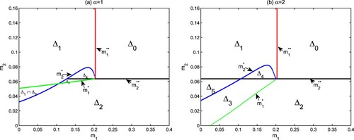
Figure 2. The parameter regions in the -plane about the survival of autotrophs and mixotrophs. Here, other parameters are from Table .
4. Autotroph and mixotroph coexistence and density
Algae are widely distributed in various aquatic ecosystems, ranging from lakes, rivers to oceans. The coexistence of autotrophic algae and mixotrophic algae in the intraguild predation structure plays an important role in maintaining algal biodiversity and explaining the phytoplankton paradox [Citation14, Citation24, Citation25]. The coexistence mechanism can be significantly influenced by some biotic and abiotic factors, such as the structure of functional response functions, light intensity and nutrients input. It is meaningful to investigate the influence of these factors on the coexistence of autotrophs and mixotrophs. The algal biomass density is an essential indicator for forewarning algal blooms and evaluating water quality. Another purpose of the section is to consider the effects of environmental factors on the biomass density of autotrophs and mixotrophs.
In the following discussion, some numerical simulations are done to explore the coexistence and biomass density of autotrophs and mixotrophs based on parameters in biologically reasonable ranges listed in Table . Here, there are several parameter values that we assume. Due to the simultaneous autotrophic and heterotrophic activities of mixotrophs, they have lower nutrient and light absorption rates than autotrophs. Hence it is biologically reasonable to assume that ,
. The value of β is chosen from the autotrophic biomass density in our numerical simulations. The research background of the current paper is a well-mixed aquatic environment such as shallow lakes or epilimnion. This means that L = 10 m is also consistent with the realistic aquatic environment.
4.1. Autotroph and mixotroph coexistence
We first consider the effect of different functional responses on the coexistence of autotrophs and mixotrophs. To facilitate the following analysis, in view of Theorems 3.2, 3.3, 3.4 and 3.6, we denote
and divide the parameter space of
as follows:
Here,
are the critical loss rates for autotrophs and mixotrophs from extinction to survival in an aquatic ecosystem.
The functional responses are the most important component between predator and prey. Choose (Equation2(2)
(2) ) and let
(10)
(10) We consider two classical functional responses:
(Holling type II functional response) and
(Holling type III functional response). Figure shows the parameter regions in the
-plane about survival of autotrophs and mixotrophs for different Holling type functional responses. The extinction of both autotrophs and mixotrophs with nutrients reaching the fixed external dissolved nutrients
(
) can occur if autotrophic and mixotrophic loss rates are very large (see
and Theorem 3.2). The coexistence of autotrophs and dissolved nutrients with the extinction of mixotrophs (
), and the coexistence of mixotrophs and dissolved nutrients with the extinction of autotrophs (
) are both possible outcomes of model (Equation3
(3)
(3) ) for different parameter ranges (see
,
and Theorems 3.3, 3.4). Autotrophs, mixotrophs and nutrients appear together in aquatic ecosystems (see
and Theorem 3.6). The numerical simulations indicate that there are bistable structures in regions
and
, and autotrophs and mixotrophs also coexist in
.
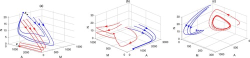
Model (Equation3(3)
(3) ) has extremely complex dynamic behaviours. From Figure , one can see that there are two bistable cases for different values α. The first case is that the semi-trivial steady states
and
are bistable in
with respect to different initial values and
(see Figure (a)). This is due to the competition between autotrophs and mixotrophs for light and nutrients. Another case is that
and
or an oscillatory periodic solution are bistable in
for
(see Figure (b,c)). This suggests that the initial values of the model can also determine the coexistence of autotrophs and mixotrophs. From the point of view of actual ecosystems, the initial biomass of autotrophic algae and mixotrophic algae directly affects the final results of competition and coexistence between them.
Figure 3. Bistability of model (Equation3(3)
(3) ). (a)
and
are bistable in
for
,
,
; (b)
and
are bistable in
for
,
,
; (c)
and a positive periodic solution are bistable in
for
,
,
. Here, other parameters are from Table .
By comparing (a) and (b) in Figure , one can observe that there are similarities and many differences between Holling type II functional response () and Holling type III functional response (
). They all have four situations: algae extinction, only autotrophs, only mixotrophs and coexistence. But there are also some differences between them. One difference is that there are a bistable region
of
and
for
, and a bistable region
of
and
or a positive periodic solution for
. Another difference is that autotrophs and mixotrophs have a larger coexistence area
for
. This means that Holling III type functional response is conducive to the coexistence of autotrophs and mixotrophs under the framework of intraguild predation.
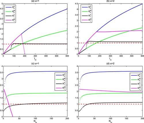
The water surface light intensity and the nutrient input concentration
are two important abiotic factors in aquatic ecosystems. They will change with the seasons and climate. Figure shows the influence of
and
on the ecological reproductive indexes
, i = 0, 1 for different Holling type functional responses. From Figure (a,c), it is found that
will increase and exceed the threshold 1 if
and
raise. While
exhibits a rapid increase above 1, followed by a rapid decrease below 1. This makes the region with
very small. On the contrary, it can be seen from Figure (b) that there is a unique threshold value about light
so that
if
. Similarly there also is a unique threshold value about nutrient
so that
if
(see Figure (d)). The above analysis shows that high light intensity
and nutrient concentration
are beneficial to the existence of autotrophs and mixotrophs for Holling III type functional response. This research also suggests that the intraguild predation structure can be used to explain the phytoplankton paradox, especially when (Equation10
(10)
(10) ) is Holling III type functional response.
Figure 4. Influence of the water surface light intensity and the nutrient input concentration
on the ecological reproductive indexes
, i = 0, 1. (a,b)
; (c,d)
. Here,
and other parameters are from Table .
4.2. Biomass density
The biomass density of autotrophic algae and mixotrophic algae as an important indicator of algal blooms is closely related to some important environmental parameters. For example, L and D are parameters relevant to water depth and movement; and
are parameters about light;
are parameters related to nutrients;
are parameters related to water temperature and organic carbon degradation; Parameter a describes the heterotrophic activity of mixotrophs. In the following study, we use the Holling type II functional response (
) and explore the effects of environmental factors in system (Equation3
(3)
(3) ) on the density of autotrophs and mixotrophs.
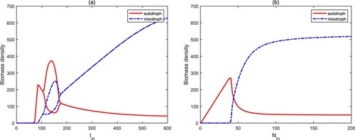
From Figure (a), one can observe that if the surface light density is very low, both autotrophic algae and mixotrophic algae will become extinct (
). As light intensity increases gradually, autotrophs can invade the aquatic ecosystems and occupy a dominant position (
). When the light intensity is high, there is a regime transition from autotrophs to mixotrophs, and mixotrophs dominate the whole aquatic ecosystems. In this process, the numerical bifurcation diagram implies that there exist two stability switches for
. Figure (b) shows a similar process for the nutrient input concentration
from
,
to
. The reason for the above phenomenons is that although high light intensity and nutrient input concentration are conducive to the growth of autotrophs and mixotrophs, the high biomass of mixotrophic algae will cause the rapid decrease of the biomass of autotrophic algae due to the predation between the two. Therefore, mixotrophic algae are more prone to blooms for high light intensity and nutrient concentration because of intraguild predation.
Figure 5. Bifurcation diagrams of autotrophs and mixotrophs for and
. Here, other parameters are from Table .
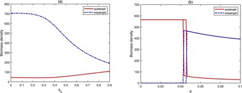
The light attenuation coefficient is used to describe the turbidity of water quality. From Figure (a), we find that the increase of
causes a positive effect on autotrophs and a negative effect on mixotrophs. This means that the clear water is more favourable for mixotrophs in the framework of intraguild predation. The attack rate a is an important parameter to assess the heterotrophic activity of mixotrophs. Figure (b) shows three stages: autotroph-only
, the bistability of
and
and the coexistence
. When the value of a is low, which implies that mixotrophs mainly carry out autotrophic activities, the biomass of autotrophs is high, but that of mixotrophs is low. This suggests that autotrophs are a powerful competitor and limit the growth of mixotrophs in an aquatic ecosystem since mixotrophs have a lower growth rate. When the attack rate a varies in high level, we observed the opposite phenomenon because of the enhancement of predation. In the bistable stage, the final biomass density of autotrophs and mixotrophs is directly determined by their initial biomass. Therefore, high heterotrophic activity raises the probability of mixotrophic algal blooms, and conversely, the possibility of autotrophic algal blooms will increase.
Figure 6. Bifurcation diagrams of autotrophs and mixotrophs for and
. Here, other parameters are from Table .
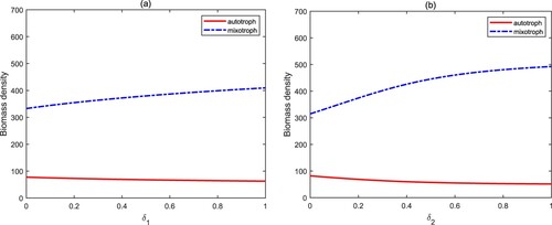
The parameter and
describe the nutrient recycling proportions, which are closely related and proportional to the degradation rate of bacterial organic carbon and the internal temperature of the water. It has been shown that the increase of the nutrient recycling proportion causes a sharp increase in the biomass of algae, and finally leads to the occurrence of algal blooms [Citation27, Citation28]. Figure exhibits a different situation from the past. The biomass density of autotrophs and mixotrophs does not change, or only slightly increases. This is mainly attributed to the intraguild predation structure between autotrophs and mixotrophs. Mixotrophs control autotrophic algae by predation. On the contrary, autotrophs suppress mixotrophic algae through competition.
Figure 7. Bifurcation diagrams of autotrophs and mixotrophs for and
. Here, other parameters are from Table .
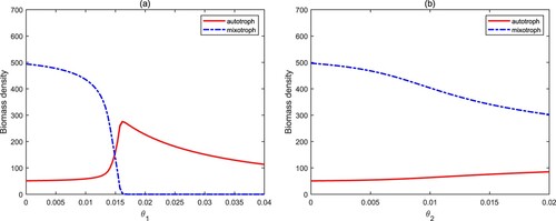
The quota of nutrients to carbon in algal cells describes the quality of algae, and it is constantly changing [Citation10, Citation11, Citation17]. From Figure (a), we find that when varies in low level, the biomass density of mixotrophs is higher than that of autotrophs when they coexist. Although the growth of autotrophs needs lower nutrients, which means that they should have higher biomass, the biomass of autotrophs did not increase significantly. This is mainly due to the predation of mixotrophs. When
increases in high level, we get an opposite result. Mixotrophs are extinct, and autotrophs have become a dominator in aquatic ecosystems. In this case, autotrophs consume more nutrients, leading to the extinction of mixotrophs through competition. In comparison,
only causes little effect on the biomass density of autotrophs and mixotrophs (see Figure (b)).
Figure 8. Bifurcation diagrams of autotrophs and mixotrophs for and
. Here, other parameters are from Table .
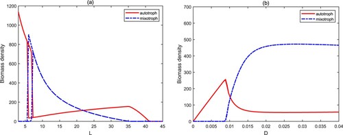
The water depth L has an important effect on the biomass density of autotrophs and mixotrophs. With the increase of the water depth L, model (Equation3(3)
(3) ) has four situations: autotroph-only
, the bistability of
and
, the coexistence
, and the extinction
(see Figure (a)). Their total biomass is gradually decreasing. It also confirms once again that the shallow aquatic systems are more prone to algal blooms. The exchange rate D characterizes the water movement, which is mainly caused by wind and the density difference of water body. A low value of D means less nutrient input. Mixotrophs are extinct since they are at a disadvantage in competing with autotrophs for nutrients. The high exchange rate (D) is conducive to the coexistence of autotrophs and mixotrophs, and mixotrophs have more biomass (see Figure (b)).
Figure 9. Bifurcation diagrams of autotrophs and mixotrophs for and
. Here, other parameters are from Table .
In summary, we let BDA represents the biomass density of autotrophic algae, and BDM represents the biomass density of mixotrophic algae. PAB characterizes the probability of autotrophic algal blooms, and PMB describes the probability of mixotrophic algal blooms. The influence of partial parameters on the growth of autotrophs and mixotrophs can be summarized in Table .
Table 2. Example of a table showing that its caption is as wide as the table itself and justified.
5. Conclusion and discussion
In this paper, we propose and investigate a mathematical model (Equation3(3)
(3) ) describing the interactions of autotrophs (autotrophic algae) and mixotrophs (mixotrophic algae) with the intragulid predation structure in a well-mixed aquatic environment. Mixotrophs compete with autotrophs for light and nutrients, and also consume micro-autotrophs. The ecological reproductive indexes for the extinction, survival and coexistence of autotrophs and mixotrophs are rigorously derived. All possible results of system (Equation3
(3)
(3) ) are described in terms of parameters
and summarized in Figure . This research indicates that the intraguild predation structure is beneficial to phytoplankton biodiversity, and provides an explanation for the phytoplankton paradox.
The different Holling type functional responses and some important environmental parameters could influence the coexistence and the biomass density of autotrophs and mixotrophs. Our results show that Holling III type functional response is conducive to the coexistence of autotrophs and mixotrophs under the intraguild predation structure. There exists the critical light intensity and the critical nutrient input concentration
that affect the coexistence of autotrophs and mixotrophs (see Figure ). The effect of environmental factors on the metabolism of autotrophs and mixotrophs is complicated (see Table ). These results are helpful for protecting water quality and evaluating algae blooms.
The coexistence mechanism of autotrophs and mixotrophs is very complex. It has stable positive steady-state solutions, periodic solutions generated by Hopf bifurcation and double Hopf bifurcations, and multiple stability switches. In the theoretical analysis, we only prove the existence of positive steady-state solutions. Rigorously proving the remaining coexistence mechanism is an interesting and important question. Ecological stoichiometry is a very important method and tool, including energy flow and element cycle [Citation10, Citation11, Citation18, Citation23]. Previous studies have considered stoichiometric autotroph–mixotroph interactions without light [Citation15, Citation16, Citation24, Citation25]. It is of interest to add stoichiometric mechanism into system (Equation3(3)
(3) ) to investigate some new findings.
The turbulence of the lake changes with the water depth [Citation26]. In the upper layer, algae mixes better since the turbulence is intense, while the turbulence is relatively small in the lower layer, and algae exhibit spatial heterogeneity. The interesting problem is to explore the interactions of autotrophs and mixotrophs with light and nutrients in a water ecosystem with spatial heterogeneity. In view of the present analysis and model (Equation3(3)
(3) ), there are more interesting ecological problems worthy of careful discussion. For example, adding dissolved inorganic carbon [Citation28], zooplankton and fishes [Citation11, Citation12] and the effect of toxic plankton species [Citation6].
Disclosure statement
No potential conflict of interest was reported by the author(s).
Additional information
Funding
References
- M. Chen, M. Fan, R. Liu, X.Y. Wang, X. Yuan, and H.P. Zhu, The dynamics of temperature and light on the growth of phytoplankton, J. Theor. Biol. 385 (2015), pp. 8–19.
- K.W. Crane and J.P. Grover, Coexistence of mixotrophs, autotrophs, and heterotrophs in planktonic microbial communities, J. Theor. Biol. 262 (2010), pp. 517–527.
- K.F. Edwards, Mixotrophy in nanoflagellates across environmental gradients in the ocean, Proc. Natl. Acad. Sci. 116 (2019), pp. 6211–6220.
- C.M. Heggerud, H. Wang, and M.A. Lewis, Transient dynamics of a stoichiometric cyanobacteria model via multiple-scale analysis, SIAM J. Appl. Math. 80 (2020), pp. 1223–1246.
- R.D. Holt and G.A. Polis, A theoretical framework for intraguild predation, Am. Nat. 149 (1997), pp. 745–764.
- S.B. Hsu, F.B. Wang, and X.Q. Zhao, A reaction-diffusion model of harmful algae and zooplankton in an ecosystem, J. Math. Anal. Appl. 451 (2017), pp. 659–677.
- J. Huisman and F.J. Weissing, Light-limited growth and competition for light in well-mixed aquatic environments: An elementary model, Ecology 75 (1994), pp. 507–520.
- J. Huisman and F.J. Weissing, Competition for nutrients and light in a mixed water column: A theoretical analysis, Am. Nat. 146 (1995), pp. 536–564.
- G.E. Hutchinson, The paradox of the plankton, Am. Nat. 95 (1961), pp. 137–145.
- X. Li, H. Wang, and Y. Kuang, Global analysis of a stoichiometric producer-grazer model with Holling type functional responses, J. Math. Biol. 63 (2011), pp. 901–932.
- I. Loladze, Y. Kuang, and J.J. Elser, Stoichiometry in producer-grazer systems: Linking energy flow with element cycling, Bull. Math. Biol. 62 (2000), pp. 1137–1162.
- D.Y. Lv, M. Fan, Y. Kang, and K. Blanco, Modeling refuge effect of submerged macrophytes in lake system, Bull. Math. Biol. 78 (2016), pp. 662–694.
- K. Mischaikow, H. Smith, and H.R. Thieme, Asymptotically autonomous semiflows: Chain recurrence and Lyapunov functions, Trans. Am. Math. Soc. 347 (1995), pp. 1669–1685.
- H.V. Moeller, M.G. Neubert, and M.D. Johnson, Intraguild predation enables coexistence of competing phytoplankton in a well-mixed water column, Ecology 100 (2019), Article ID e02874.
- H. Nie, S.B. Hsu, and F.B. Wang, Steady-state solutions of a reaction-diffusion system arising from intraguild predation and internal storage, J. Differ. Equ. 266 (2019), pp. 8459–8491.
- H. Nie, S.B. Hsu, and F.B. Wang, Global dynamics of a reaction-diffusion system with intraguild predation and internal storage, Discrete Cont. Dyn. Syst. Ser. B 25 (2020), pp. 877–901.
- A. Peace, Effects of light, nutrients, and food chain length on trophic efficiencies in simple stoichiometric aquatic food chain models, Ecol. Model. 312 (2015), pp. 125–135.
- A. Peace and H. Wang, Compensatory foraging in stoichiometric producer-grazer models, Bull. Math. Biol. 81 (2019), pp. 4932–4950.
- R. Peng and X.Q. Zhao, A nonlocal and periodic reaction–diffusion–advection model of a single phytoplankton species, J. Math. Biol. 72 (2016), pp. 755–791.
- G.A. Polis and R.D. Holt, Intraguild predation: The dynamics of complex trophic interactions, Trends Ecol. Evol. 7 (1992), pp. 151–154.
- A.B. Ryabov, L. Rudolf, and B. Blasius, Vertical distribution and composition of phytoplankton under the influence of an upper mixed layer, J. Theor. Biol. 263 (2010), pp. 120–133.
- F.R. Vasconcelos, S. Diehl, P. Rodríguez, P. Hedström, J. Karlsson, and P. Byström, Asymmetrical competition between aquatic primary producers in a warmer and browner world, Ecology97 (2016), pp. 2580–2592.
- H. Wang, H.L. Smith, Y. Kuang, and J.J. Elser, Dynamics of stoichiometric bacteria-algae interactions in the epilimnion, SIAM J. Appl. Math. 68 (2007), pp. 503–522.
- S. Wilken, J.M.H. Verspagen, S. Naus-Wiezer, E. Van Donk, and J. Huisman, Biological control of toxic cyanobacteria by mixotrophic predators: An experimental test of intraguild predation theory, Ecol. Appl. 24 (2014), pp. 1235–1249.
- S. Wilken, J.M.H. Verspagen, S. Naus-Wiezer, E. Van Donk, and J. Huisman, Comparison of predator-prey interactions with and without intraguild predation by manipulation of the nitrogen source, Oikos 123 (2014), pp. 423–432.
- A. Wüest and A. Lorke, Small-scale hydrodynamics in lakes, Annu. Rev. Fluid Mech. 35 (2003), pp. 373–412.
- J.M. Zhang, J.P. Shi, and X.Y. Chang, A mathematical model of algae growth in a pelagic-benthic coupled shallow aquatic ecosystem, J. Math. Biol. 76 (2018), pp. 1159–1193.
- J.M. Zhang, J.P. Shi, and X.Y. Chang, A model of algal growth depending on nutrients and inorganic carbon in a poorly mixed water column, J. Math. Biol. 83 (2021), p. 15.
- J.M. Zhang, J.D. Kong, J.P. Shi, and H. Wang, Phytoplankton competition for nutrients and light in a stratified lake: A mathematical model connecting epilimnion and hypolimnion, J. Nonlinear Sci. 31 (2021), p. 35.
- X.Q. Zhao, Dynamical Systems in Population Biology, Springer, New York, 2003.