Stability of a fear effect predator–prey model with mutual interference or group defense

Abstract

In this paper, we consider a fear effect predator–prey model with mutual interference or group defense. For the model with mutual interference, we show the interior equilibrium is globally stable, and the mutual interference can stabilize the predator–prey system. For the model with group defense, we discuss the singular dynamics around the origin and the occurrence of Hopf bifurcation, and find that there is a separatrix curve near the origin such that the orbits above which tend to the origin and the orbits below which tend to limit cycle or the interior equilibrium.

Keywords:

• Fear effect
• mutual interference
• group defense
• Hopf bifurcation
• predator–prey

1. Introduction

Most of predator–prey systems take into account only the direct killing by predators [2,7,11,12,19,20,22,29,30,32,34,35,38,40], but not the cost of fear effect, which is considered to be more powerful than direct predation. Zanette et al. [36] showed that the bird reduce 40% less offspring by predation fears. Therefore, Wang et al. [25] investigated the following predator–prey system with fear effect (1) $\begin{array}{rl}{x}^{\prime }(t)& =axF(f,y)-\mathrm{d}x-b{x}^2-mxy,\\ y^{\prime }(t)& =nmxy-ey.\end{array}$(1) They considered the cost of fear into prey reproduction. a is the birth rate of prey; d is the natural death rate of prey; f is the level of fear; $F(f,y)$ is the cost of anti-predator defence due to fear. Here $F(f,y)$ can be reasonably assumed (2) $\begin{array}{rl}& F(0,y)=1,F(f,0)=1,\underset{f\to +\mathrm{\infty }}{lim}F(f,y)=0,\\ & \underset{y\to +\mathrm{\infty }}{lim}F(f,y)=0,\frac{\mathrm{\partial }F(f,y)}{\mathrm{\partial }f}<0,\frac{\mathrm{\partial }F(f,y)}{\mathrm{\partial }y}<0.\end{array}$(2) They showed the fear effect has no impact on the stability of system (1(1) $\begin{array}{rl}{x}^{\prime }(t)& =axF(f,y)-\mathrm{d}x-b{x}^2-mxy,\\ y^{\prime }(t)& =nmxy-ey.\end{array}$(1) ). But for the Holling type II of system (1(1) $\begin{array}{rl}{x}^{\prime }(t)& =axF(f,y)-\mathrm{d}x-b{x}^2-mxy,\\ y^{\prime }(t)& =nmxy-ey.\end{array}$(1) ), they showed that the fear can make the system become stable. Cong et al. [5] investigated a three-species food chain model with fear effect and showed that the fear effect can change the model from a chaotic state to a stable state. Based on system (1(1) $\begin{array}{rl}{x}^{\prime }(t)& =axF(f,y)-\mathrm{d}x-b{x}^2-mxy,\\ y^{\prime }(t)& =nmxy-ey.\end{array}$(1) ), Pal et al. [14] discussed the stability, Hopf-bifurcation and Bogdanov–Takens bifurcation of a predator–prey system with fear effect and hunting cooperation. Zhang et al. [37] investigated the influence of fear effect and prey refuge on the stability of a predator–prey system and showed that the fear effect can stabilize the system. Tiwari et al. [23] considered a predator–prey model with Beddington–DeAngelis functional response and the fear effect into prey, and discussed the stability and bifurcations of the system. By incorporating spatial memory and pregnancy period, Wang et al. [27] performed the detailed bifurcation analysis, and their results indicated that the memory ability and pregnancy cycle of prey play significant roles in the spatiotemporal dynamics of prey–predator models in an intimidatory environment. Sasmal [18] studied the following predator–prey model with fear effect and Allee effect (3) $\begin{array}{rl}{x}^{\prime }(t)& =rx(1-\frac{x}{k})(x-\delta )\frac{1}{1+fy}-axy,\\ y^{\prime }(t)& =a\alpha xy-my,\end{array}$(3) where $0<\delta <k$ expresses a strong Allee effect; $\frac{1}{1+fv}$ is one type of fear effect, which satisfies (2(2) $\begin{array}{rl}& F(0,y)=1,F(f,0)=1,\underset{f\to +\mathrm{\infty }}{lim}F(f,y)=0,\\ & \underset{y\to +\mathrm{\infty }}{lim}F(f,y)=0,\frac{\mathrm{\partial }F(f,y)}{\mathrm{\partial }f}<0,\frac{\mathrm{\partial }F(f,y)}{\mathrm{\partial }y}<0.\end{array}$(2) ). Due to the increase of the fear effect, the author showed the decrease of per-capita growth rate and the multistability of the system. From more results about fear effect, see [16,21,26].

In 1975, Hassell's research of the capturing behaviour between larvae of Plodia interpunctella and Colorado potato beetles showed that the predators will leave each other when they encountered. Thus this mutual interference phenomenon can reduce the search efficiency of predators. This functional response is particularly applicable to systems in patchy environments where parasites tend to cluster in some patches rather than others. Hassell [10] introduced a mutual interference constant $\theta (0<\theta <1)$ into a Volterra model. Although models considering predator interference have different mathematical expressions, the same qualitative results are given [3]. That is when predator interference is low, increasing predator interference has a positive effect on the asymptotic stability of system. Further, Freedman [9] analysed the stability of the mutual interference system. Wang and Zhu [28] considered the stability of a delayed impulsive prey-predator system with mutual interference. Xiao and Li [31] considered a predator–prey model (1(1) $\begin{array}{rl}{x}^{\prime }(t)& =axF(f,y)-\mathrm{d}x-b{x}^2-mxy,\\ y^{\prime }(t)& =nmxy-ey.\end{array}$(1) ) with mutual interference (4) $\begin{array}{rl}{x}^{\prime }(t)& =axF(f,y)-\mathrm{d}x-b{x}^2-mx{y}^{\theta },\\ y^{\prime }(t)& =nmx{y}^{\theta }-ey,\end{array}$(4) where $0<\theta <1$. When $\theta =1$, system (4(4) $\begin{array}{rl}{x}^{\prime }(t)& =axF(f,y)-\mathrm{d}x-b{x}^2-mx{y}^{\theta },\\ y^{\prime }(t)& =nmx{y}^{\theta }-ey,\end{array}$(4) ) is reduced to model (1(1) $\begin{array}{rl}{x}^{\prime }(t)& =axF(f,y)-\mathrm{d}x-b{x}^2-mxy,\\ y^{\prime }(t)& =nmxy-ey.\end{array}$(1) ). Notice that the positive equilibrium of system (1(1) $\begin{array}{rl}{x}^{\prime }(t)& =axF(f,y)-\mathrm{d}x-b{x}^2-mxy,\\ y^{\prime }(t)& =nmxy-ey.\end{array}$(1) ) is unstable, but when considering system (1(1) $\begin{array}{rl}{x}^{\prime }(t)& =axF(f,y)-\mathrm{d}x-b{x}^2-mxy,\\ y^{\prime }(t)& =nmxy-ey.\end{array}$(1) ) with mutual interference, that is system (4(4) $\begin{array}{rl}{x}^{\prime }(t)& =axF(f,y)-\mathrm{d}x-b{x}^2-mx{y}^{\theta },\\ y^{\prime }(t)& =nmx{y}^{\theta }-ey,\end{array}$(4) ), this unstable positive equilibrium becomes stable. Hence, the mutual interference can stabilize the predator–prey system.

In nature, prey gathers together in herds to protect themselves from predator. That is prey allows the weakest individuals to occupy the inside of the herd for defensive purposes, leaving the healthier and stronger prey around it. Then in the predator–prey model, in which prey exhibits herd behaviour, predator interacts with prey along the outer corridor of the prey group. By assuming the prey individuals at the herd boundary is proportional to the square root of the area, Braza [4] and Ajraldi et . al [1] studied the models with square root of the prey population, which represent the predator interacts with the prey along the outer corridor of the herd of prey. Due to the square root term, Braza [4] showed the origin is more subtle. That is, the first quadrant is divided into two parts by a separatrix curve near the origin. The orbits above the separatrix curve will tend to origin, but the orbits below the separatrix curve will leave the origin. This phenomenon also appears in the predator-prey with ratio-dependent functional responses [7,32]. Salman [17] considered the stability of a discrete-time system with square root functional responses. When considering the interaction between the prey and the predator in both cases 2D and 3D herd shapes, a new functional response in the θ power of prey has been proposed. The authors [24] and [33] proposed a functional response in terms of the $\theta (0<\theta <1)$ power of prey, which is more general than [1,4]. More precisely, they studied the following model: $\begin{array}{rl}{x}^{\prime }& =rx(1-\frac{x}{K})-a{x}^{\theta }y,\\ y^{\prime }& =ae{x}^{\theta }y-my,\end{array}$where $0<\theta <1$. When $\theta =\frac{1}{2}$, the functional responses of the above system are reduced to square root functional responses [1,4]. The authors [24,33] found that the solution behaviour near the origin is singularity and can occur Hopf bifurcation. Djilali [8] extended the model in [24,33] to functional response with Holling-II.

In this paper, we study the following model: (5) $\begin{array}{rl}{x}^{\prime }& =rx(1-\frac{x}{K})\frac{1}{1+fy}-pxy,\\ y^{\prime }& =hpxy-ey,\end{array}$(5) where all parameters of system (5(5) $\begin{array}{rl}{x}^{\prime }& =rx(1-\frac{x}{K})\frac{1}{1+fy}-pxy,\\ y^{\prime }& =hpxy-ey,\end{array}$(5) ) are positive constants; r is the birth rate of prey; K is the carrying capacity; p is the capture rate; h is the conversion efficiency; e is the death rate of predator; $\frac{1}{1+fy}$ is the cost of anti-predator defence due to fear [18,25]; f is the level of fear; the fear effect can lead to the decrease of per-capita growth rate. Let $\begin{array}{rl}& \overline{x}=\frac{x}{K},\overline{y}=\frac{py}{r},\overline{t}=rt,\\ & \overline{f}=\frac{fr}{p},a=\frac{hpK}{r},d=\frac{e}{r}.\end{array}$Dropping the bar, system (5(5) $\begin{array}{rl}{x}^{\prime }& =rx(1-\frac{x}{K})\frac{1}{1+fy}-pxy,\\ y^{\prime }& =hpxy-ey,\end{array}$(5) ) is reduced to (6) $\begin{array}{rl}{x}^{\prime }& =\frac{x(1-x)}{1+fy}-xy\triangleq P_1(x,y),\\ y^{\prime }& =axy-dy\triangleq Q_1(x,y).\end{array}$(6) Based on the above discussion on mutual interference and group defense, we expect to discuss the effect of mutual interference and group defense on the dynamical behaviours of the system (6(6) $\begin{array}{rl}{x}^{\prime }& =\frac{x(1-x)}{1+fy}-xy\triangleq P_1(x,y),\\ y^{\prime }& =axy-dy\triangleq Q_1(x,y).\end{array}$(6) ). Therefore, we also respectively study (7) $\begin{array}{rl}{x}^{\prime }& =\frac{x(1-x)}{1+fy}-x{y}^{{\theta }_1}\triangleq P_2(x,y),\\ y^{\prime }& =ax{y}^{{\theta }_1}-dy\triangleq Q_2(x,y),\end{array}$(7) where ${\theta }_1$ $(0<{\theta }_1<1)$ is the mutual interference constant; and (8) $\begin{array}{rl}{x}^{\prime }& =\frac{x(1-x)}{1+fy}-x^{{\theta }_2}y,\\ y^{\prime }& =a{x}^{{\theta }_2}y-dy,\end{array}$(8) where ${\theta }_2$ $(0<{\theta }_2<1)$ is the group defense constant. The organization of this paper is as follows: In Section 2, the stability of system (6(6) $\begin{array}{rl}{x}^{\prime }& =\frac{x(1-x)}{1+fy}-xy\triangleq P_1(x,y),\\ y^{\prime }& =axy-dy\triangleq Q_1(x,y).\end{array}$(6) ) is investigated. In Sections 3 and 4, the dynamic behaviours of systems (7(7) $\begin{array}{rl}{x}^{\prime }& =\frac{x(1-x)}{1+fy}-x{y}^{{\theta }_1}\triangleq P_2(x,y),\\ y^{\prime }& =ax{y}^{{\theta }_1}-dy\triangleq Q_2(x,y),\end{array}$(7) ) and (8(8) $\begin{array}{rl}{x}^{\prime }& =\frac{x(1-x)}{1+fy}-x^{{\theta }_2}y,\\ y^{\prime }& =a{x}^{{\theta }_2}y-dy,\end{array}$(8) ) are respectively investigated. In Section 5, the influences of fear effect, mutual interference and group defense on population density are respectively discussed. Finally, a brief discussion is given.

2. Fear effect predator–prey model (6)

The following lemma shows solutions of system (6(6) $\begin{array}{rl}{x}^{\prime }& =\frac{x(1-x)}{1+fy}-xy\triangleq P_1(x,y),\\ y^{\prime }& =axy-dy\triangleq Q_1(x,y).\end{array}$(6) ) are positive and uniformly bounded.

Lemma 2.1

Any solution of system (6(6) $\begin{array}{rl}{x}^{\prime }& =\frac{x(1-x)}{1+fy}-xy\triangleq P_1(x,y),\\ y^{\prime }& =axy-dy\triangleq Q_1(x,y).\end{array}$(6) ) satisfies $0<x(t)<1$ and $0<x(t)+\mathrm{d}y(t)<\frac{a(d+1{)}^2}{4d}$ for all large t.

Proof. Obviously, solutions of system (6(6) $\begin{array}{rl}{x}^{\prime }& =\frac{x(1-x)}{1+fy}-xy\triangleq P_1(x,y),\\ y^{\prime }& =axy-dy\triangleq Q_1(x,y).\end{array}$(6) ) are positive. If $x(t)\ge 1$, it follows from the first equation of system (6(6) $\begin{array}{rl}{x}^{\prime }& =\frac{x(1-x)}{1+fy}-xy\triangleq P_1(x,y),\\ y^{\prime }& =axy-dy\triangleq Q_1(x,y).\end{array}$(6) ) that $x^{\prime }(t)<0$. Then $0<x(t)<1$ for all large t.

Define a function $V(x,y)=ax+y$. Differentiating V along the solution of system (6(6) $\begin{array}{rl}{x}^{\prime }& =\frac{x(1-x)}{1+fy}-xy\triangleq P_1(x,y),\\ y^{\prime }& =axy-dy\triangleq Q_1(x,y).\end{array}$(6) ) for large t, we have $V^{\prime }(x,y)=\frac{ax(1-x)}{1+fy}-\mathrm{d}y\le ax(1-x)-\mathrm{d}y,$that is $V^{\prime }(x,y)+dV(x,y)\le ax(d+1-x)\le \frac{a(d+1{)}^2}{4}.$Hence, $V(x,y)\le \frac{a(d+1{)}^2}{4d}$ for large t, i.e. $0<x(t)+\mathrm{d}y(t)<\frac{a(d+1{)}^2}{4d}$ for all large t. This completes the proof of Lemma 2.1.

Now, we consider the existence and stability of the equilibria of system (6(6) $\begin{array}{rl}{x}^{\prime }& =\frac{x(1-x)}{1+fy}-xy\triangleq P_1(x,y),\\ y^{\prime }& =axy-dy\triangleq Q_1(x,y).\end{array}$(6) ). There always exist a trivial equilibrium $E_0^1(0,0)$ and a boundary equilibria $E_1^1(1,0)$. By computation, system (6(6) $\begin{array}{rl}{x}^{\prime }& =\frac{x(1-x)}{1+fy}-xy\triangleq P_1(x,y),\\ y^{\prime }& =axy-dy\triangleq Q_1(x,y).\end{array}$(6) ) has a positive equilibrium $E_1^{\ast }(x_1^{\ast },y_1^{\ast })$ if a>d, where $x_1^{\ast }=\frac{d}{a}$ and $y_1^{\ast }=\frac{-1+\sqrt{1+4f(1-x_1^{\ast })}}{2f}$.

Lemma 2.2

(1)	$E_0^1$ is unstable.
(2)	If $a\le d$, then $E_1^1$ is locally asymptotically stable. If a>d, $E_1^1$ is unstable.

Proof.

The eigenvalues of $E_0^1$ are ${\lambda }_1=1$ and ${\lambda }_2=-d$, so $E_0^1$ is unstable. Note that the eigenvalues at $E_1^1$ are ${\lambda }_1=-1$ and ${\lambda }_2=a-d$, then $E_1^1$ is unstable if a>d and stable if a<d.

When a = d, i.e. ${\lambda }_2=0$, translating $E_1^1$ to the origin by letting $x_1=x-1,y_1=y$, we obtain the Taylor expansions of system (6(6) $\begin{array}{rl}{x}^{\prime }& =\frac{x(1-x)}{1+fy}-xy\triangleq P_1(x,y),\\ y^{\prime }& =axy-dy\triangleq Q_1(x,y).\end{array}$(6) ) as follows: $\begin{array}{rl}{x}_1^{\prime }& =-x_1-y_1-x_1^2+(f-1)x_1{y}_1+O(|x_1,y_1{|}^3),\\ y_1^{\prime }& =\mathrm{d}{x}_1{y}_1+O(|x_1,y_1{|}^3).\end{array}$Further, letting $x_2=x_1+y_1,y_2=y_1$, rewriting $x_2,y_2$ as x, y again, we have $\begin{array}{rl}{x}^{\prime }& =-x-x^2+(1+f)xy-f{y}^2+O(|x,y{|}^3),\\ y^{\prime }& =-\mathrm{d}{y}^2+\mathrm{d}xy+O(|x,y{|}^3).\end{array}$It follows from Theorem 7.1 in Zhang et al. [39] that $E_1^1$ is a saddle-node, which includes a stable parabolic sector. Then $E_1^1$ is stable if $a\le d$. This completes the proof of Lemma 2.2.

Theorem 2.1

(1)	If $a\le d$, then $E_1^1$ is globally asymptotically stable.
(2)	If a>d, then $E_1^{\ast }$ is globally asymptotically stable.

Proof.

(1) From Lemma 2.2, if $a\le d$, $E_0^1$ is unstable, $E_1^1$ is locally asymptotically stable and $E_1^{\ast }$ does not exist. Assume that system (6(6) $\begin{array}{rl}{x}^{\prime }& =\frac{x(1-x)}{1+fy}-xy\triangleq P_1(x,y),\\ y^{\prime }& =axy-dy\triangleq Q_1(x,y).\end{array}$(6) ) has a closed orbit, then there must exist an equilibrium in the interior of the closed orbit, which is impossible. Therefore, system (6(6) $\begin{array}{rl}{x}^{\prime }& =\frac{x(1-x)}{1+fy}-xy\triangleq P_1(x,y),\\ y^{\prime }& =axy-dy\triangleq Q_1(x,y).\end{array}$(6) ) does not exist a limit cycle. Hence, $E_1^1$ is globally asymptotically stable.

(2) If a>d, $E_0^1$ and $E_1^1$ are unstable. The Jacobin matrix at $E_1^{\ast }$ is calculated as $J(E_1^{\ast })=\left[\begin{array}{cc}-{\displaystyle \frac{x_1^{\ast }}{1+f{y}_1^{\ast }}}& -x_1^{\ast }(1+{\displaystyle \frac{f(1-x_1^{\ast })}{(1+f{y}_1^{\ast }{)}^2}})\\ a{y}_1^{\ast }& 0\end{array}\right].$Noting that $x_1^{\ast }<1$, the eigenvalues at $E_1^{\ast }$ satisfies ${\lambda }_1{\lambda }_2=a{x}_1^{\ast }{y}_1^{\ast }(1+\frac{f(1-x_1^{\ast })}{(1+f{y}_1^{\ast }{)}^2})>0$ and ${\lambda }_1+{\lambda }_2=-\frac{x_1^{\ast }}{1+f{y}_1^{\ast }}<0.$ Then $E_1^{\ast }$ is stable if a>d. We consider a Dulac function $B(x,y)=x^{-1}{y}^{-1}$, then $\frac{\mathrm{\partial }(B{P}_1)}{\mathrm{\partial }x}+\frac{\mathrm{\partial }(B{Q}_1)}{\mathrm{\partial }y}=-\frac{1}{y(1+fy)}<0,$for all x>0 and y>0. It follows from the Dulac theorem that there is no closed orbit. Hence, $E_1^{\ast }$ is globally asymptotically stable. This completes the proof of Theorem 2.1.

3. Fear effect predator–prey model with mutual interference

In this section, we consider the global asymptotic stability of system (7(7) $\begin{array}{rl}{x}^{\prime }& =\frac{x(1-x)}{1+fy}-x{y}^{{\theta }_1}\triangleq P_2(x,y),\\ y^{\prime }& =ax{y}^{{\theta }_1}-dy\triangleq Q_2(x,y),\end{array}$(7) ). Obviously, system (7(7) $\begin{array}{rl}{x}^{\prime }& =\frac{x(1-x)}{1+fy}-x{y}^{{\theta }_1}\triangleq P_2(x,y),\\ y^{\prime }& =ax{y}^{{\theta }_1}-dy\triangleq Q_2(x,y),\end{array}$(7) ) has a trivial equilibrium $E_0^2(0,0)$ and a boundary equilibria $E_1^2(1,0)$. Next we show that system (7(7) $\begin{array}{rl}{x}^{\prime }& =\frac{x(1-x)}{1+fy}-x{y}^{{\theta }_1}\triangleq P_2(x,y),\\ y^{\prime }& =ax{y}^{{\theta }_1}-dy\triangleq Q_2(x,y),\end{array}$(7) ) has a unique positive equilibrium $E_2^{\ast }(x_1^{\ast },y_1^{\ast })$.

Lemma 3.1

System (7(7) $\begin{array}{rl}{x}^{\prime }& =\frac{x(1-x)}{1+fy}-x{y}^{{\theta }_1}\triangleq P_2(x,y),\\ y^{\prime }& =ax{y}^{{\theta }_1}-dy\triangleq Q_2(x,y),\end{array}$(7) ) always has a unique positive equilibrium $E_2^{\ast }(x_1^{\ast },y_1^{\ast })$.

Proof.

The prey isocline of system (7(7) $\begin{array}{rl}{x}^{\prime }& =\frac{x(1-x)}{1+fy}-x{y}^{{\theta }_1}\triangleq P_2(x,y),\\ y^{\prime }& =ax{y}^{{\theta }_1}-dy\triangleq Q_2(x,y),\end{array}$(7) ) is $l_1$: $f{y}^{{\theta }_1+1}+y^{{\theta }_1}-(1-x)=0$. Let x = 0, then $H(y)=f{y}^{{\theta }_1+1}+y^{{\theta }_1}-1$. Notice that $H(0)=-1,H(+\mathrm{\infty })=+\mathrm{\infty },H^{\prime }(y)>0$, then there exists a unique $y_0>0$ such that $H(y_0)=0$. Since $\frac{\mathrm{d}y}{\mathrm{d}x}=-\frac{1}{f({\theta }_1+1)y^{{\theta }_1}+{\theta }_1{y}^{{\theta }_1-1}}<0$, $l_1$ decreases with respect to x, which passes through $(1,0)$ and $(0,y_0)$.

The predator isocline of system (7(7) $\begin{array}{rl}{x}^{\prime }& =\frac{x(1-x)}{1+fy}-x{y}^{{\theta }_1}\triangleq P_2(x,y),\\ y^{\prime }& =ax{y}^{{\theta }_1}-dy\triangleq Q_2(x,y),\end{array}$(7) ) is $l_2$: $y^{1-{\theta }_1}=\frac{ax}{d}$. Hence, $l_2$ increases with respect to x, which passes through $(0,0)$.

It follows from the above discussion that $l_1$ and $l_2$ have a unique interior intersection point in the first quadrant. Therefore, system (7(7) $\begin{array}{rl}{x}^{\prime }& =\frac{x(1-x)}{1+fy}-x{y}^{{\theta }_1}\triangleq P_2(x,y),\\ y^{\prime }& =ax{y}^{{\theta }_1}-dy\triangleq Q_2(x,y),\end{array}$(7) ) admits a unique positive equilibrium $E_2^{\ast }(x_2^{\ast },y_2^{\ast })$. This completes the proof of Lemma 3.1.

Theorem 3.1

$E_2^{\ast }$ of system (7(7) $\begin{array}{rl}{x}^{\prime }& =\frac{x(1-x)}{1+fy}-x{y}^{{\theta }_1}\triangleq P_2(x,y),\\ y^{\prime }& =ax{y}^{{\theta }_1}-dy\triangleq Q_2(x,y),\end{array}$(7) ) is globally asymptotically stable.

Proof.

By calculation, we have $\begin{array}{rl}& \frac{\mathrm{\partial }P(0,0)}{\mathrm{\partial }x}=\underset{x\to 0}{lim}\frac{P(x,0)-P(0,0)}{x}=1,\frac{\mathrm{\partial }P(0,0)}{\mathrm{\partial }y}=\underset{y\to 0}{lim}\frac{P(0,y)-P(0,0)}{y}=0,\\ & \frac{\mathrm{\partial }Q(0,0)}{\mathrm{\partial }x}=\underset{x\to 0}{lim}\frac{Q(x,0)-Q(0,0)}{x}=0,\frac{\mathrm{\partial }Q(0,0)}{\mathrm{\partial }y}=\underset{y\to 0}{lim}\frac{Q(0,y)-Q(0,0)}{y}=-d.\end{array}$Then, the eigenvalues corresponding to $E_0^2$ are ${\lambda }_1=1$ and ${\lambda }_2=-d$, then $E_0^2$ is unstable.

Translating $E_1^2$ to the origin by letting $x_1=x-1,y_1=y,\mathrm{d}{t}_1=\frac{1}{1+fy}\mathrm{d}t$, we have (9) $\begin{array}{rl}{x}_1^{\prime }& =-(x_1+1)(x_1+(1+f{y}_1)y_1^{{\theta }_1}),\\ y_1^{\prime }& =(1+f{y}_1)(a(x_1+1)y_1^{{\theta }_1}-\mathrm{d}{y}_1).\end{array}$(9) Denote $\alpha =\frac{1}{{\theta }_1}$, then $\alpha >1$. Further, taking the following scalings $x_2=x_1,y_2=y_1^{\frac{1}{\alpha }},\mathrm{d}{t}_2=\alpha y_1\mathrm{d}{t}_1$, and rewriting $x_2,y_2,t_2$ as x, y, t respectively again, system (9(9) $\begin{array}{rl}{x}_1^{\prime }& =-(x_1+1)(x_1+(1+f{y}_1)y_1^{{\theta }_1}),\\ y_1^{\prime }& =(1+f{y}_1)(a(x_1+1)y_1^{{\theta }_1}-\mathrm{d}{y}_1).\end{array}$(9) ) becomes (10) $\begin{array}{rl}{x}^{\prime }& =-\alpha y^{\alpha +1}-\alpha x{y}^{\alpha }+O(|x,y{|}^{\alpha +2}),\\ y^{\prime }& =a{y}^2-\mathrm{d}{y}^{\alpha +1}-ax{y}^2+O(|x,y{|}^{\alpha +2}).\end{array}$(10) Define $x=r\cos \phi$ and $y=r\sin \phi$, then system (10(10) $\begin{array}{rl}{x}^{\prime }& =-\alpha y^{\alpha +1}-\alpha x{y}^{\alpha }+O(|x,y{|}^{\alpha +2}),\\ y^{\prime }& =a{y}^2-\mathrm{d}{y}^{\alpha +1}-ax{y}^2+O(|x,y{|}^{\alpha +2}).\end{array}$(10) ) can be rewritten as $r\frac{\mathrm{d}\phi }{\mathrm{d}r}=\frac{F(\phi )+o(1)}{G(\phi )+o(1)},$where $F(\phi )=a\cos \phi {\sin }^2\phi$ and $G(\phi )=a{\sin }^3\phi$. Hence, ${\phi }_1=\frac{\pi }{2}$ is a exceptional direction. Note that $F^{\prime }(\frac{\pi }{2})<0$ and $G(\frac{\pi }{2})>0$, i.e. $F^{\prime }(\frac{\pi }{2})G(\frac{\pi }{2})<0$. Therefore, the normal sector of ${\phi }_1$ is second type, and there is a unique orbit of system (10(10) $\begin{array}{rl}{x}^{\prime }& =-\alpha y^{\alpha +1}-\alpha x{y}^{\alpha }+O(|x,y{|}^{\alpha +2}),\\ y^{\prime }& =a{y}^2-\mathrm{d}{y}^{\alpha +1}-ax{y}^2+O(|x,y{|}^{\alpha +2}).\end{array}$(10) ) along the exceptional direction ${\phi }_1=\frac{\pi }{2}$ starting from the origin. Hence, in the first quadrant, there exists a unique orbit of system (7(7) $\begin{array}{rl}{x}^{\prime }& =\frac{x(1-x)}{1+fy}-x{y}^{{\theta }_1}\triangleq P_2(x,y),\\ y^{\prime }& =ax{y}^{{\theta }_1}-dy\triangleq Q_2(x,y),\end{array}$(7) ) along the line x = 1 starting from $E_1^2$. Note that $x^{\prime }{|}_{y=0}=x(1-x)$ and $y^{\prime }{|}_{y=0}=0$, then the x-axis is an orbit of system (7(7) $\begin{array}{rl}{x}^{\prime }& =\frac{x(1-x)}{1+fy}-x{y}^{{\theta }_1}\triangleq P_2(x,y),\\ y^{\prime }& =ax{y}^{{\theta }_1}-dy\triangleq Q_2(x,y),\end{array}$(7) ). Finally, it follows from the above analysis that $E_1^2$ is unstable.

The Jacobin matrix at $E_2^{\ast }$ is calculated as $J(E_2^{\ast })=\left[\begin{array}{cc}-{\displaystyle \frac{x_2^{\ast }}{1+f{y}_2^{\ast }}}& -x_1^{\ast }({\theta }_1(y_2^{\ast }{)}^{{\theta }_1-1}+{\displaystyle \frac{f(1-x_2^{\ast })}{(1+f{y}_2^{\ast }{)}^2}})\\ a(y_2^{\ast }{)}^{{\theta }_1}& -(1-{\theta }_1)a{x}_2^{\ast }(y_2^{\ast }{)}^{{\theta }_1-1}\end{array}\right].$Noting that $x_2^{\ast }<1$, the eigenvalues at $E_2^{\ast }$ satisfy ${\lambda }_1{\lambda }_2>0$ and ${\lambda }_1+{\lambda }_2<0$, that is $E_2^{\ast }$ is stable. Define a Dulac function $B(x,y)=x^{-1}{y}^{-1}$, then $\frac{\mathrm{\partial }(B{P}_1)}{\mathrm{\partial }x}+\frac{\mathrm{\partial }(B{Q}_1)}{\mathrm{\partial }y}=-\frac{1}{y(1+fy)}-a(1-{\theta }_1)y^{{\theta }_1-2}<0,$for all x>0 and y>0. Then there is no closed orbit in system (7(7) $\begin{array}{rl}{x}^{\prime }& =\frac{x(1-x)}{1+fy}-x{y}^{{\theta }_1}\triangleq P_2(x,y),\\ y^{\prime }& =ax{y}^{{\theta }_1}-dy\triangleq Q_2(x,y),\end{array}$(7) ). Hence, $E_2^{\ast }$ is globally asymptotically stable. This completes the proof of Theorem 3.1.

Remark 3.1

From the proof of Theorem 3.1, both $E_0^2$ and $E_1^2$ are unstable.

4. Fear effect predator–prey model with group defense

In this section, we consider system (7(7) $\begin{array}{rl}{x}^{\prime }& =\frac{x(1-x)}{1+fy}-x{y}^{{\theta }_1}\triangleq P_2(x,y),\\ y^{\prime }& =ax{y}^{{\theta }_1}-dy\triangleq Q_2(x,y),\end{array}$(7) ). There always exist a trivial equilibrium $E_0^3(0,0)$ and a boundary equilibria $E_1^3(1,0)$. By simple computation, if a>d, system (8(8) $\begin{array}{rl}{x}^{\prime }& =\frac{x(1-x)}{1+fy}-x^{{\theta }_2}y,\\ y^{\prime }& =a{x}^{{\theta }_2}y-dy,\end{array}$(8) ) has a positive equilibrium $E_3^{\ast }(x_3^{\ast },y_3^{\ast })$, where $x_3^{\ast }={\left(\frac{d}{a}\right)}^{\frac{1}{{\theta }_2}}\text{ and}{y}_3^{\ast }=\frac{-1+\sqrt{1+4f(x_3^{\ast }{)}^{1-{\theta }_2}(1-x_3^{\ast })}}{2f}.$Stimulated by the works of [4,24,33], we have the following theorem about the singular dynamics of system (8(8) $\begin{array}{rl}{x}^{\prime }& =\frac{x(1-x)}{1+fy}-x^{{\theta }_2}y,\\ y^{\prime }& =a{x}^{{\theta }_2}y-dy,\end{array}$(8) ) around the origin.

Theorem 4.1

Let $(x(t),y(t))$ be any positive solution of system (8(8) $\begin{array}{rl}{x}^{\prime }& =\frac{x(1-x)}{1+fy}-x^{{\theta }_2}y,\\ y^{\prime }& =a{x}^{{\theta }_2}y-dy,\end{array}$(8) ) with initial condition $x(0)>0$ and $y(0)>0$. Then there exists a separatrix curve L near the origin, which passes through the origin. If $(x(0),y(0))$ is above the L, then system (8(8) $\begin{array}{rl}{x}^{\prime }& =\frac{x(1-x)}{1+fy}-x^{{\theta }_2}y,\\ y^{\prime }& =a{x}^{{\theta }_2}y-dy,\end{array}$(8) ) is extinct.

Proof.

Note that the solution of system (8(8) $\begin{array}{rl}{x}^{\prime }& =\frac{x(1-x)}{1+fy}-x^{{\theta }_2}y,\\ y^{\prime }& =a{x}^{{\theta }_2}y-dy,\end{array}$(8) ) is positive. By the second equation of system (8(8) $\begin{array}{rl}{x}^{\prime }& =\frac{x(1-x)}{1+fy}-x^{{\theta }_2}y,\\ y^{\prime }& =a{x}^{{\theta }_2}y-dy,\end{array}$(8) ), we have $y^{\prime }\ge -\mathrm{d}y.$Consider an equation $u^{\prime }=-\mathrm{d}u$satisfying $y_0=y(0)=u(0)$, then $u(t)=y_0{e}^{-\mathrm{d}t}$. By the comparison theorem, we have $y(t)\ge u(t)$ for t>0, that is $y(t)\ge y_0{e}^{-\mathrm{d}t}\mathrm{for}\mathrm{all}t>0.$From the first equation of system (8(8) $\begin{array}{rl}{x}^{\prime }& =\frac{x(1-x)}{1+fy}-x^{{\theta }_2}y,\\ y^{\prime }& =a{x}^{{\theta }_2}y-dy,\end{array}$(8) ), we have $x^{\prime }\le x-x^{{\theta }_2}y\le x-y_0{e}^{-\mathrm{d}t}{x}^{{\theta }_2}.$Considering the following Bernoulli equation: $v^{\prime }=v-y_0{e}^{-\mathrm{d}t}{v}^{{\theta }_2}$with $x_0=x(0)=v(0)$, we have $x(t)\le v(t)$ for t>0. Solving the above Bernoulli equation, we have $v^{1-{\theta }_2}(t)=(x_0^{1-{\theta }_2}-\frac{y_0(1-{\theta }_2)}{d+1-{\theta }_2})e^{(1-{\theta }_2)t}+\frac{y_0(1-{\theta }_2)}{d+1-{\theta }_2}{e}^{-\mathrm{d}t}.$Hence, $x^{1-{\theta }_2}(t)\le (x_0^{1-{\theta }_2}-\frac{y_0(1-{\theta }_2)}{d+1-{\theta }_2})e^{(1-{\theta }_2)t}+\frac{y_0(1-{\theta }_2)}{d+1-{\theta }_2}{e}^{-\mathrm{d}t}\mathrm{for}\mathrm{all}t>0.$If $y_0=\frac{d+1-{\theta }_2}{1-{\theta }_2}{x}_0^{1-{\theta }_2}$, then $\underset{t\to +\mathrm{\infty }}{lim}x(t)=0$. If $y_0>\frac{d+1-{\theta }_2}{1-{\theta }_2}{x}_0^{1-{\theta }_2}$, then there exists a $t^{\ast }>0$ such that $x(t^{\ast })=0$. Hence, when $y_0\ge \frac{d+1-{\theta }_2}{1-{\theta }_2}{x}_0^{1-{\theta }_2}$, the prey x is extinct.

There exists a positive ε such that $a{\epsilon }^{{\theta }_2}-d<0$. Since x is extinct, there exists a $t_1$ such that $x(t)\le \epsilon$ for $t>t_1$. Form the first equation of system (8(8) $\begin{array}{rl}{x}^{\prime }& =\frac{x(1-x)}{1+fy}-x^{{\theta }_2}y,\\ y^{\prime }& =a{x}^{{\theta }_2}y-dy,\end{array}$(8) ), we have $y^{\prime }\le (a{\epsilon }^{{\theta }_2}-d)y\mathrm{for}\mathrm{all}t>t_1.$Similarly, we have $y(t)\le y(t_1)e^{(a{\epsilon }^{{\theta }_2}-d)(t-t_1)}.$Then $\underset{t\to +\mathrm{\infty }}{lim}y(t)=0.$Hence, there exists a separatrix curve L below $y=\frac{d+1-{\theta }_2}{1-{\theta }_2}{x}^{1-{\theta }_2}$. If the initial condition $(x(0),y(0))$ of system (8(8) $\begin{array}{rl}{x}^{\prime }& =\frac{x(1-x)}{1+fy}-x^{{\theta }_2}y,\\ y^{\prime }& =a{x}^{{\theta }_2}y-dy,\end{array}$(8) ) is above the L, then system (8(8) $\begin{array}{rl}{x}^{\prime }& =\frac{x(1-x)}{1+fy}-x^{{\theta }_2}y,\\ y^{\prime }& =a{x}^{{\theta }_2}y-dy,\end{array}$(8) ) is extinct. This completes the proof of Theorem 4.1.

Remark 4.1

Since the singularity of the origin, then the origin cannot be linearized. If we use the method in the proof of Theorem 3.1, then the origin is a saddle which is incorrect. If the initial condition of system (8(8) $\begin{array}{rl}{x}^{\prime }& =\frac{x(1-x)}{1+fy}-x^{{\theta }_2}y,\\ y^{\prime }& =a{x}^{{\theta }_2}y-dy,\end{array}$(8) ) above the separatrix curve L, the orbits will intersect with y-axis, and tend to the origin along the y-axis.

Theorem 4.2

(1)	If $a\le d$, then $E_1^3$ is locally asymptotically stable.
(2)	If a>d, then $E_1^3$ is unstable.

Proof.

The eigenvalues at $E_1^3$ are ${\lambda }_1=-1$ and ${\lambda }_2=a-d$, then $E_1^1$ is unstable if a>d and stable if a<d.

If a = d, then ${\lambda }_2=0$. Translating $E_1^3$ to the origin by X = x−1, Y = y, rewriting X and Y as x and y respectively, we obtain the Taylor expansions of system (8(8) $\begin{array}{rl}{x}^{\prime }& =\frac{x(1-x)}{1+fy}-x^{{\theta }_2}y,\\ y^{\prime }& =a{x}^{{\theta }_2}y-dy,\end{array}$(8) ) as follows: (11) $\begin{array}{rl}{x}^{\prime }& =-x-y-x^2+(f-{\theta }_2)xy+O(|x,y{|}^3),\\ y^{\prime }& =\mathrm{d}{\theta }_{2}xy+O(|x,y{|}^3).\end{array}$(11) Letting X = x + y, Y = y, rewriting X and Y as x and y respectively, system (11(11) $\begin{array}{rl}{x}^{\prime }& =-x-y-x^2+(f-{\theta }_2)xy+O(|x,y{|}^3),\\ y^{\prime }& =\mathrm{d}{\theta }_{2}xy+O(|x,y{|}^3).\end{array}$(11) ) can be written as $\begin{array}{rl}{x}^{\prime }& =-x-x^2+(2+f-{\theta }_2)xy+({\theta }_2-1-f)y^2+O(|x,y{|}^3),\\ y^{\prime }& =-\mathrm{d}{\theta }_2{y}^2+\mathrm{d}{\theta }_{2}xy+O(|x,y{|}^3).\end{array}$It follows from Theorem 7.1 in Zhang et al, [39] that $E_1^3$ is a saddle-node, which includes a stable parabolic sector. Then $E_1^3$ is stable if $a\le d$. This completes the proof of Theorem 4.2.

Now, we show the stability of $E_3^{\ast }$. The Jacobin matrix at $E_3^{\ast }$ is calculated as $\begin{array}{l}J(E_3^{\ast })=\left[\begin{array}{cc}{x}_3^{\ast }(-{\displaystyle \frac{1}{1+f{y}_3^{\ast }}+(1-{\theta }_2)(x_3^{\ast }{)}^{{\theta }_2-2}{y}_3^{\ast }})& -(x_3^{\ast }{)}^{{\theta }_2}-{\displaystyle \frac{f{x}_3^{\ast }(1-x_3^{\ast })}{(1+f{y}_3^{\ast }{)}^2}}\\ a{\theta }_2(x_3^{\ast }{)}^{{\theta }_2-1}{y}_3^{\ast }& 0\end{array}\right].\end{array}$It is easy to obtain that $\det (J(E_3^{\ast }))>0$ and $\mathrm{tr}(J(E_3^{\ast }))=\frac{(1-{\theta }_2)-(2-{\theta }_2)x_3^{\ast }}{1+f{y}_3^{\ast }}$.

Define $d^{\ast }=d{\left(\frac{2-{\theta }_2}{1-{\theta }_2}\right)}^{{\theta }_2}.$Hence, if $d<a<d^{\ast }$, that is $\mathrm{tr}(J(E_3^{\ast }))<0$, then $E_3^{\ast }$ is stable. If $a>d^{\ast }$, that is $\mathrm{tr}(J(E_3^{\ast }))>0$, then $E_3^{\ast }$ is unstable.

Noting that $\mathrm{tr}(J(E_3^{\ast })){|}_{a=d^{\ast }}=0$, we can check the transversality condition $\frac{\mathrm{d}(\mathrm{tr}(J(E_3^{\ast })))}{\mathrm{d}t}{|}_{a=d^{\ast }}=\frac{(2-{\theta }_2)x_3^{\ast }}{a{\theta }_2(1+f{y}_3^{\ast })}>0.$Hence, system (8(8) $\begin{array}{rl}{x}^{\prime }& =\frac{x(1-x)}{1+fy}-x^{{\theta }_2}y,\\ y^{\prime }& =a{x}^{{\theta }_2}y-dy,\end{array}$(8) ) undergoes a Hopf bifurcation at $a=d^{\ast }$. With the increase of a, tr$(J(E_3^{\ast }))$ changes sign from negative to positive, which implies $E_3^{\ast }$ loses its stability and Hopf bifurcation occurs.

Now we determine the stability of the limit cycle by calculating the first Lyapunov coefficient. Since the group defense is defined by the ${\theta }_2(0<{\theta }_2<1)$ power of prey and the expression of $E_3^{\ast }$ is complicated, it is difficult to calculate the first Lyapunov coefficient. For simplicity, stimulated by the technique of [6,13], we make the following scaling for system (8(8) $\begin{array}{rl}{x}^{\prime }& =\frac{x(1-x)}{1+fy}-x^{{\theta }_2}y,\\ y^{\prime }& =a{x}^{{\theta }_2}y-dy,\end{array}$(8) ): $\begin{array}{rl}\overline{x}& =\frac{x}{x_3^{\ast }},\overline{y}=\frac{y}{y_3^{\ast }},\overline{t}=x_3^{\ast }t,b=\frac{1}{x_3^{\ast }},\\ \overline{f}& =f{y}_3^{\ast },p=\frac{y_3^{\ast }}{(x_3^{\ast }{)}^{2-{\theta }_2}},\overline{a}=a(x_3^{\ast }{)}^{{\theta }_2-1},\overline{d}=\frac{d}{x_3^{\ast }}.\end{array}$Note that $a(x_3^{\ast }{)}^{{\theta }_2}=d$ and $x_3^{\ast }<1$, then $\overline{a}=\overline{d}$ and b>1, respectively. Dropping the bar, system (8(8) $\begin{array}{rl}{x}^{\prime }& =\frac{x(1-x)}{1+fy}-x^{{\theta }_2}y,\\ y^{\prime }& =a{x}^{{\theta }_2}y-dy,\end{array}$(8) ) is reduced to (12) $\begin{array}{rl}{x}^{\prime }& =\frac{x(b-x)}{1+fy}-p{x}^{{\theta }_2}y,\\ y^{\prime }& =a{x}^{{\theta }_2}y-ay.\end{array}$(12) $E_3^{\ast }(x_3^{\ast },y_3^{\ast })$ of system (8(8) $\begin{array}{rl}{x}^{\prime }& =\frac{x(1-x)}{1+fy}-x^{{\theta }_2}y,\\ y^{\prime }& =a{x}^{{\theta }_2}y-dy,\end{array}$(8) ) is transformed to $E^{\ast }(1,1)$ of system (12(12) $\begin{array}{rl}{x}^{\prime }& =\frac{x(b-x)}{1+fy}-p{x}^{{\theta }_2}y,\\ y^{\prime }& =a{x}^{{\theta }_2}y-ay.\end{array}$(12) ). Hence, we have $p=\frac{b-1}{1+f}.$Then system (12(12) $\begin{array}{rl}{x}^{\prime }& =\frac{x(b-x)}{1+fy}-p{x}^{{\theta }_2}y,\\ y^{\prime }& =a{x}^{{\theta }_2}y-ay.\end{array}$(12) ) can be written as follows: (13) $\begin{array}{rl}{x}^{\prime }& =\frac{x(b-x)}{1+fy}-\frac{b-1}{1+f}{x}^{{\theta }_2}y,\\ y^{\prime }& =a{x}^{{\theta }_2}y-ay.\end{array}$(13) Obviously system (13(13) $\begin{array}{rl}{x}^{\prime }& =\frac{x(b-x)}{1+fy}-\frac{b-1}{1+f}{x}^{{\theta }_2}y,\\ y^{\prime }& =a{x}^{{\theta }_2}y-ay.\end{array}$(13) ) has the same topological structure as that of system (8(8) $\begin{array}{rl}{x}^{\prime }& =\frac{x(1-x)}{1+fy}-x^{{\theta }_2}y,\\ y^{\prime }& =a{x}^{{\theta }_2}y-dy,\end{array}$(8) ), then we calculate the first Lyapunov coefficient of system (13(13) $\begin{array}{rl}{x}^{\prime }& =\frac{x(b-x)}{1+fy}-\frac{b-1}{1+f}{x}^{{\theta }_2}y,\\ y^{\prime }& =a{x}^{{\theta }_2}y-ay.\end{array}$(13) ) to determine the stability of the limit cycle. The Jacobian matrix of system (13(13) $\begin{array}{rl}{x}^{\prime }& =\frac{x(b-x)}{1+fy}-\frac{b-1}{1+f}{x}^{{\theta }_2}y,\\ y^{\prime }& =a{x}^{{\theta }_2}y-ay.\end{array}$(13) ) at $E^{\ast }(1,1)$ takes the form $\begin{array}{l}J(E^{\ast })=\left[\begin{array}{cc}{\displaystyle \frac{(1-{\theta }_2)(b-1)-1}{1+f}}& -{\displaystyle \frac{(b-1)(2f+1)}{1+f}}\\ a{\theta }_2& 0\end{array}\right].\end{array}$Then $\det (J(E^{\ast }))=\frac{a{\theta }_2(b-1)(2f+1)}{1+f}>0$and $\mathrm{tr}(J(E^{\ast }))=\frac{(1-{\theta }_2)(b-1)-1}{1+f}.$Let $b^{\ast }=1+\frac{1}{1-{\theta }_2}$, then we obtain $\mathrm{tr}(J(E^{\ast })){|}_{b=b^{\ast }}=0$. We have the transversality condition as follows: ${\frac{\mathrm{d}(\mathrm{tr}(J(E^{\ast })))}{\mathrm{d}t}|}_{b=b^{\ast }}=\frac{1-{\theta }_2}{1+f}>0.$Hence, system (13(13) $\begin{array}{rl}{x}^{\prime }& =\frac{x(b-x)}{1+fy}-\frac{b-1}{1+f}{x}^{{\theta }_2}y,\\ y^{\prime }& =a{x}^{{\theta }_2}y-ay.\end{array}$(13) ) undergoes a Hopf bifurcation at $b=b^{\ast }$ (i.e. $a=d^{\ast }$ of system (8(8) $\begin{array}{rl}{x}^{\prime }& =\frac{x(1-x)}{1+fy}-x^{{\theta }_2}y,\\ y^{\prime }& =a{x}^{{\theta }_2}y-dy,\end{array}$(8) )).

Letting X = x−1, Y = y−1, rewriting X and Y as x and y respectively, we obtain the Taylor expansions of system (13(13) $\begin{array}{rl}{x}^{\prime }& =\frac{x(b-x)}{1+fy}-\frac{b-1}{1+f}{x}^{{\theta }_2}y,\\ y^{\prime }& =a{x}^{{\theta }_2}y-ay.\end{array}$(13) ) as follows: (14) $\{\begin{array}{ll}\dot{x}& =a_{10}x+a_{01}y+a_{20}{x}^2+a_{11}xy+a_{02}{y}^2+a_{30}{x}^3\\ & +a_{21}{x}^{2}y+a_{12}x{y}^2+a_{03}{y}^3,\\ \dot{y}& =b_{10}x+b_{01}y+b_{20}{x}^2+b_{11}xy+b_{02}{y}^2+b_{30}{x}^3\\ & +b_{21}{x}^{2}y+b_{12}x{y}^2+b_{03}{y}^3,\end{array}$(14) where $a_{10}=0,a_{01}=-\frac{2f+1}{(1-{\theta }_2)(1+f{)}^2},a_{20}=\frac{{\theta }_2-2}{2(1+f)},a_{11}=-\frac{(2f+1){\theta }_2}{(1+f{)}^2(1-{\theta }_2)},$ $a_{02}=\frac{f^2}{(1-{\theta }_2)(1+f{)}^3},a_{30}=\frac{({\theta }_2-2){\theta }_2}{6(1+f)},a_{12}=\frac{f^2{\theta }_2}{(1-{\theta }_2)(1+f{)}^3},a_{21}=\frac{f{\theta }_2+2f+{\theta }_2}{2(1+f{)}^2},$ $a_{03}=-\frac{f^3}{(1+f{)}^4(1-{\theta }_2)},b_{10}=a{\theta }_2,b_{01}=0,b_{20}=\frac{1}{2}a{\theta }_2({\theta }_2-1),b_{11}=a{\theta }_2,b_{30}=\frac{1}{6}a{\theta }_2({\theta }_2-1)({\theta }_2-2),b_{21}=\frac{1}{2}a{\theta }_2({\theta }_2-1),b_{02}=b_{12}=b_{03}=0.$

The first-order Lyapunov number (Perko [15]) can be expressed as follows: $\begin{array}{rl}{l}_1& =\frac{-3\pi }{2a_{01}{\mathrm{\Phi }}^{3/2}}\{[a_{10}{b}_{10}(a_{11}^2+a_{11}{b}_{02}+a_{02}{b}_{11})+a_{10}{a}_{01}(b_{11}^2+a_{20}{b}_{11}+a_{11}{b}_{02})\\ & +b_{10}^2(a_{11}{a}_{02}+2a_{02}{b}_{02})-2a_{10}{b}_{10}(b_{02}^2-a_{20}{a}_{02})-2a_{10}{a}_{01}(a_{20}^2-b_{20}{b}_{02})\\ & -a_{01}^2(2a_{20}{b}_{20}+b_{11}{b}_{20})+(a_{01}{b}_{10}-2a_{10}^2)(b_{11}{b}_{02}-a_{11}{a}_{20})]\\ & -(a_{10}^2+a_{01}{b}_{10})[3(b_{10}{b}_{03}-a_{01}{a}_{30})+2a_{10}(a_{21}+b_{12})+(b_{10}{a}_{12}-a_{01}{b}_{21})]\}\\ & =-\frac{3\pi a{\theta }_2(2f+1)(2-{\theta }_2)}{4{\mathrm{\Phi }}^{3/4}(1+f{)}^3},\end{array}$where $\mathrm{\Phi }=\det (J(E^{\ast }))$.

Obviously $l_1<0$, system (13(13) $\begin{array}{rl}{x}^{\prime }& =\frac{x(b-x)}{1+fy}-\frac{b-1}{1+f}{x}^{{\theta }_2}y,\\ y^{\prime }& =a{x}^{{\theta }_2}y-ay.\end{array}$(13) ) undergoes a supercritical Hopf bifurcation at $E^{\ast }(1,1)$ and exists a stable limit cycle around $E^{\ast }$.

From the above discussion, we have the following theorem.

Theorem 4.3

Let $d^{\ast }=d{\left(\frac{2-{\theta }_2}{1-{\theta }_2}\right)}^{{\theta }_2}$, then the following conclusions hold.

(1)	If $d<a<d^{\ast }$, then $E_3^{\ast }$ is locally asymptotically stable.
(2)	If $a>d^{\ast }$, then $E_3^{\ast }$ is unstable.
(3)	If $a=d^{\ast }$, then system (4.1) undergoes a supercritical Hopf bifurcation at $E_3^{\ast }$ and exists a stable limit cycle around $E_3^{\ast }$.

Notice that $f{({\theta }_2)=(\frac{2-{\theta }_2}{1-{\theta }_2})}^{{\theta }_2}$ is monotonically increasing when $0<{\theta }_2<1$, hence $a=d^{\ast }$ exists a unique positive solution ${\theta }_2^{\ast }\in (0,1)$. From Theorem 4.1, we can easily obtain the following corollary.

Corollary 4.1

Assume that a>d, then the following conclusions hold.

(1)	If ${\theta }_2^{\ast }<{\theta }_2<1$, then $E_3^{\ast }$ is locally asymptotically stable.
(2)	If $0<{\theta }_2<{\theta }_2^{\ast }$, then $E_3^{\ast }$ is unstable.
(3)	If ${\theta }_2={\theta }_2^{\ast }$, then system (4.1) undergoes a supercritical Hopf bifurcation at $E_3^{\ast }$ and exists a stable limit cycle around $E_3^{\ast }$.

5. The influences of fear effect, mutual interference and group defense

5.1. The influence of fear effect on population density

Obviously, the fear effect has no impact on the stability of systems (6(6) $\begin{array}{rl}{x}^{\prime }& =\frac{x(1-x)}{1+fy}-xy\triangleq P_1(x,y),\\ y^{\prime }& =axy-dy\triangleq Q_1(x,y).\end{array}$(6) ) – (8(8) $\begin{array}{rl}{x}^{\prime }& =\frac{x(1-x)}{1+fy}-x^{{\theta }_2}y,\\ y^{\prime }& =a{x}^{{\theta }_2}y-dy,\end{array}$(8) ) and the prey density at the positive equilibrium of systems (6(6) $\begin{array}{rl}{x}^{\prime }& =\frac{x(1-x)}{1+fy}-xy\triangleq P_1(x,y),\\ y^{\prime }& =axy-dy\triangleq Q_1(x,y).\end{array}$(6) ) and (8(8) $\begin{array}{rl}{x}^{\prime }& =\frac{x(1-x)}{1+fy}-x^{{\theta }_2}y,\\ y^{\prime }& =a{x}^{{\theta }_2}y-dy,\end{array}$(8) ). Now we discuss the influence of the fear effect on the predator density at the positive equilibrium of systems (6(6) $\begin{array}{rl}{x}^{\prime }& =\frac{x(1-x)}{1+fy}-xy\triangleq P_1(x,y),\\ y^{\prime }& =axy-dy\triangleq Q_1(x,y).\end{array}$(6) ) and (8(8) $\begin{array}{rl}{x}^{\prime }& =\frac{x(1-x)}{1+fy}-x^{{\theta }_2}y,\\ y^{\prime }& =a{x}^{{\theta }_2}y-dy,\end{array}$(8) ). Let $\begin{array}{rl}{H}_1& =(1-x_1^{\ast })>0,{\mathrm{\Delta }}_1=1+4f{H}_1,H_3=(x_3^{\ast }{)}^{1-{\theta }_2}(1-x_3^{\ast })>0\text{ and}\\ {\mathrm{\Delta }}_3& =1+4f{H}_3.\end{array}$By computation, we obtain $\frac{\mathrm{\partial }{y}_i^{\ast }}{\mathrm{\partial }f}=-\frac{2H_i^2}{\sqrt{{\mathrm{\Delta }}_i}(\sqrt{{\mathrm{\Delta }}_i}+1+2f{H}_i)}<0,i=1,3.$Then the fear effect will change the density of predator population at the positive equilibrium of systems (6(6) $\begin{array}{rl}{x}^{\prime }& =\frac{x(1-x)}{1+fy}-xy\triangleq P_1(x,y),\\ y^{\prime }& =axy-dy\triangleq Q_1(x,y).\end{array}$(6) ) and (8(8) $\begin{array}{rl}{x}^{\prime }& =\frac{x(1-x)}{1+fy}-x^{{\theta }_2}y,\\ y^{\prime }& =a{x}^{{\theta }_2}y-dy,\end{array}$(8) ), which decreases with the increase of fear effect.

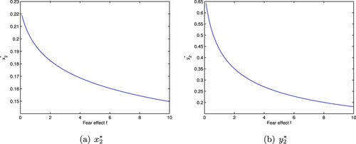
Next we study the influence of the fear effect on the positive equilibrium of system (7(7) $\begin{array}{rl}{x}^{\prime }& =\frac{x(1-x)}{1+fy}-x{y}^{{\theta }_1}\triangleq P_2(x,y),\\ y^{\prime }& =ax{y}^{{\theta }_1}-dy\triangleq Q_2(x,y),\end{array}$(7) ). Denote $\begin{array}{rl}F(x_2^{\ast },y_2^{\ast },f)& =\frac{1-x_2^{\ast }}{1+f{y}_2^{\ast }}-(y_2^{\ast }{)}^{{\theta }_1},\\ G(x_2^{\ast },y_2^{\ast },f)& =a{x}_2^{\ast }(y_2^{\ast }{)}^{{\theta }_1-1}-d.\end{array}$Then the positive equilibrium $E_2^{\ast }$ satisfies $F(x_2^{\ast },y_2^{\ast },f)=0$ and $G(x_2^{\ast },y_2^{\ast },f)=0$. By simple computation, we have $\begin{array}{rl}& J=\frac{\mathrm{\partial }(F,G)}{\mathrm{\partial }(x_2^{\ast },y_2^{\ast })}=\frac{a(y_2^{\ast }{)}^{{\theta }_1-2}((1-{\theta }_1)x_2^{\ast }+f(y_2^{\ast }{)}^{{\theta }_1+1})}{1+f{y}_2^{\ast }}+a{\theta }_1(y_2^{\ast }{)}^{2{\theta }_1-2}>0,\\ & J_1=\frac{\mathrm{\partial }(F,G)}{\mathrm{\partial }(f,y_2^{\ast })}=\frac{a(1-{\theta }_1)x_2^{\ast }(y_2^{\ast }{)}^{2{\theta }_1-1}}{1+f{y}_2^{\ast }}>0,\\ & J_2=\frac{\mathrm{\partial }(F,G)}{\mathrm{\partial }(x_2^{\ast },f)}=\frac{a(y_2^{\ast }{)}^{2{\theta }_1}}{1+f{y}_2^{\ast }}>0,\end{array}$that is, $\frac{\mathrm{d}{x}_2^{\ast }}{\mathrm{d}f}=-\frac{J_1}{J}<0,\frac{\mathrm{d}{y}_2^{\ast }}{\mathrm{d}f}=-\frac{J_2}{J}<0.$Hence, with the increase of fear level f, the value of $E_2^{\ast }$ decreases. Then we show that increasing the fear effect can decrease the predator and prey densities at the positive equilibrium, that is, fear effect can lead to the decrease of the predator and prey population (Figure 1).

Figure 1. The positive equilibrium $E_2^{\ast }$ of system (7(7) $\begin{array}{rl}{x}^{\prime }& =\frac{x(1-x)}{1+fy}-x{y}^{{\theta }_1}\triangleq P_2(x,y),\\ y^{\prime }& =ax{y}^{{\theta }_1}-dy\triangleq Q_2(x,y),\end{array}$(7) ) with $a=4,d=1,{\theta }_1=0.7$. (a) $x_2^{\ast }$ (b) $y_2^{\ast }$

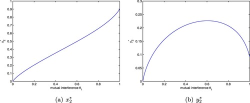
5.2. The influence of mutual interference on population density

Theorem 3.1 shows that the positive equilibrium of system (7(7) $\begin{array}{rl}{x}^{\prime }& =\frac{x(1-x)}{1+fy}-x{y}^{{\theta }_1}\triangleq P_2(x,y),\\ y^{\prime }& =ax{y}^{{\theta }_1}-dy\triangleq Q_2(x,y),\end{array}$(7) ) is globally stable unconditionally, that is, the mutual interference strengthens the stability of the system. Next we discuss the influence of mutual interference on population density.

Similarly to the analysis of the above subsection, we can easily obtain $\begin{array}{rl}& J_3=\frac{\mathrm{\partial }(F,G)}{\mathrm{\partial }({\theta }_1,y_2^{\ast })}=[(1-{\theta }_1)(y_2^{\ast }{)}^{{\theta }_1-1}+\frac{d}{a{x}_2^{\ast }}(\frac{f{y}_2^{\ast }}{1+f{y}_2^{\ast }}+{\theta }_1)]d\ln y_2^{\ast },\\ & J_4=\frac{\mathrm{\partial }(F,G)}{\mathrm{\partial }(x_2^{\ast },{\theta }_1)}=\frac{(1-2x_2^{\ast })d\ln y_2^{\ast }}{x_2^{\ast }(1+f{y}_2^{\ast })}.\end{array}$We can observe from $\frac{1-x_2^{\ast }}{1+f{y}_2^{\ast }}-(y_2^{\ast }{)}^{{\theta }_1}=0$ that $y_2^{\ast }<1$, that is $\ln y_2^{\ast }<0$. This implies $\frac{\mathrm{d}{x}_2^{\ast }}{\mathrm{d}{\theta }_1}=-\frac{J_3}{J}>0,\frac{\mathrm{d}{y}_2^{\ast }}{\mathrm{d}{\theta }_1}=-\frac{J_4}{J},$where J is given in Section 5.1. Obviously, $x_2^{\ast }$ increases with the increase of ${\theta }_1$ (Figure 2 a); meanwhile, $y_2^{\ast }$ increases with the increase of ${\theta }_1$ when $x_2^{\ast }<\frac{1}{2}$, and $y_2^{\ast }$ decreases with the increase of ${\theta }_1$ when $x_2^{\ast }>\frac{1}{2}$ (Figure 2 b). Therefore when the prey density is relatively small, $y_2^{\ast }$ increases as ${\theta }_1$ increases, that is the mutual interference constant ${\theta }_1$ has less influence on the capturing behaviour of the predator; but for the fact that the increase of ${\theta }_1$ can result in the increase of the prey density, when the prey density becomes relatively large, the effect of mutual interference on the capturing behaviour becomes stronger, which leads to the decrease of the predator density.

Figure 2. The positive equilibrium $E_2^{\ast }$ of system (7(7) $\begin{array}{rl}{x}^{\prime }& =\frac{x(1-x)}{1+fy}-x{y}^{{\theta }_1}\triangleq P_2(x,y),\\ y^{\prime }& =ax{y}^{{\theta }_1}-dy\triangleq Q_2(x,y),\end{array}$(7) ) with $a=2,d=1.8,f=1$. (a) $x_2^{\ast }$ and (b) $y_2^{\ast }$.

5.3. The influence of group defense on population density

Assume that a>d, then system (8(8) $\begin{array}{rl}{x}^{\prime }& =\frac{x(1-x)}{1+fy}-x^{{\theta }_2}y,\\ y^{\prime }& =a{x}^{{\theta }_2}y-dy,\end{array}$(8) ) has a positive equilibrium $E_3^{\ast }(x_3^{\ast },y_3^{\ast })$. Next we discuss the influence of group defense on population density under a>d. By calculation, we can easily obtain $\frac{\mathrm{d}{x}_3^{\ast }}{\mathrm{d}{\theta }_2}=\frac{x_3^{\ast }}{{\theta }_2^2}\ln \left(\frac{a}{d}\right)>0,\frac{\mathrm{d}{y}_3^{\ast }}{\mathrm{d}{\theta }_2}=\frac{a(1-2x_3^{\ast })}{d\sqrt{{△}_3}}\frac{\mathrm{d}{x}_3^{\ast }}{\mathrm{d}{\theta }_2},\text{when}a>d,$where ${△}_3$ is defined in Section 5.1. Obviously $x_3^{\ast }$ is monotonically increasing with respective to ${\theta }_2$ (Figures 3 a and 4a), hence $1-2x_3^{\ast }=0$ exists a unique positive solution ${\theta }_2^{\ast }=\ln (\frac{a}{d})/\ln 2$. This means when $0<{\theta }_2<{\theta }_2^{\ast }$, $1-2x_3^{\ast }>0$, and when ${\theta }_2^{\ast }<{\theta }_2<1$, $1-2x_3^{\ast }<0$. Next we consider two cases.

Figure 3. The positive equilibrium $E_3^{\ast }$ of system (8(8) $\begin{array}{rl}{x}^{\prime }& =\frac{x(1-x)}{1+fy}-x^{{\theta }_2}y,\\ y^{\prime }& =a{x}^{{\theta }_2}y-dy,\end{array}$(8) ) with $a=2,d=0.7,f=1$. (a) $x_3^{\ast }$ and (b) $y_3^{\ast }$.

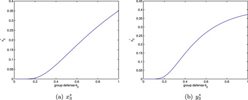
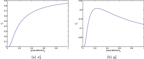
Figure 4. The positive equilibrium $E_3^{\ast }$ of system (8(8) $\begin{array}{rl}{x}^{\prime }& =\frac{x(1-x)}{1+fy}-x^{{\theta }_2}y,\\ y^{\prime }& =a{x}^{{\theta }_2}y-dy,\end{array}$(8) ) with $a=2,d=1.7,f=1,$ where ${\theta }_2^{\ast }=0.2345$. (a) $x_3^{\ast }$ and (b) $y_3^{\ast }$.

Case 1: If $a\ge 2d$, that is ${\theta }_2^{\ast }\ge 1$, which together with $0<{\theta }_2<1$ implies $1-2x_3^{\ast }>0$, then $\frac{\mathrm{d}{y}_3^{\ast }}{\mathrm{d}{\theta }_2}>0$ (Figure 3 b).

Case 2: If d<a<2d, that is $0<{\theta }_2^{\ast }<1$, then $\frac{\mathrm{d}{y}_3^{\ast }}{\mathrm{d}{\theta }_2}>0$ if $0<{\theta }_2<{\theta }_2^{\ast }$; $\frac{\mathrm{d}{y}_3^{\ast }}{\mathrm{d}{\theta }_2}<0$ if ${\theta }_2^{\ast }<{\theta }_2<1$ (Figure 4 b).

The above analysis shows that the group defense is beneficial to the density of the prey at the positive equilibrium of system (8(8) $\begin{array}{rl}{x}^{\prime }& =\frac{x(1-x)}{1+fy}-x^{{\theta }_2}y,\\ y^{\prime }& =a{x}^{{\theta }_2}y-dy,\end{array}$(8) ). For the predator, when the capture rate is large enough which can result in a large enough a, or the group defense constant is relatively small, the group defense has less influence on the capturing behaviour of the predator; but if the capture rate is relatively small, the group defense plays an important role on the capturing behaviour of the predator, the density of the predator at the positive equilibrium decreases with the increase of ${\theta }_2$.

6. Conclusion

In this paper, we considered a fear effect predator–prey model with mutual interference or group defense and studied the stability and Hopf bifurcation of the system. The stability property of system (6(6) $\begin{array}{rl}{x}^{\prime }& =\frac{x(1-x)}{1+fy}-xy\triangleq P_1(x,y),\\ y^{\prime }& =axy-dy\triangleq Q_1(x,y).\end{array}$(6) ) is simple. If $a\le d$, $E_1^1$ is globally asymptotically stable (Figure 5 a–b). If a>d, $E_1^{\ast }$ is globally asymptotically stable (Figure 5 c). Considering the original coefficients of system (5(5) $\begin{array}{rl}{x}^{\prime }& =rx(1-\frac{x}{K})\frac{1}{1+fy}-pxy,\\ y^{\prime }& =hpxy-ey,\end{array}$(5) ), $a\le d$ is equivalent to $K\le \frac{e}{hp}$. Form Figure 6, if $a\le d$, that is the carrying capacity K of prey is small enough, predator will be extinct, while prey will survive. If a>d, that is the carrying capacity K of prey is large enough, predator and prey can coexist. However, the cost of fear effect has no impact on the stability of system (6(6) $\begin{array}{rl}{x}^{\prime }& =\frac{x(1-x)}{1+fy}-xy\triangleq P_1(x,y),\\ y^{\prime }& =axy-dy\triangleq Q_1(x,y).\end{array}$(6) ), which is in accord with the predator–prey model with the linear functional response [25]. However, the mutual interference or group defense can change the stability of system (6(6) $\begin{array}{rl}{x}^{\prime }& =\frac{x(1-x)}{1+fy}-xy\triangleq P_1(x,y),\\ y^{\prime }& =axy-dy\triangleq Q_1(x,y).\end{array}$(6) ).

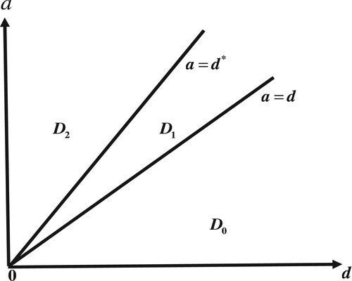
Figure 5. Fear effect predator–prey model (6(6) $\begin{array}{rl}{x}^{\prime }& =\frac{x(1-x)}{1+fy}-xy\triangleq P_1(x,y),\\ y^{\prime }& =axy-dy\triangleq Q_1(x,y).\end{array}$(6) ) with f = 3, d = 0.15. (a) a = 0.1<d, (b) a = d = 0.15 and (c) a = 0.2>d.

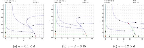
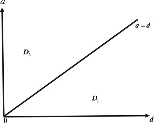
Figure 6. Bifurcation diagrams of system (6(6) $\begin{array}{rl}{x}^{\prime }& =\frac{x(1-x)}{1+fy}-xy\triangleq P_1(x,y),\\ y^{\prime }& =axy-dy\triangleq Q_1(x,y).\end{array}$(6) ). In region $D_2$, $E_1^{\ast }$ is globally asymptotically stable. In region $D_1$, $E_1^1$ is globally asymptotically stable.

By introducing the parameter ${\theta }_1$ $(0<{\theta }_1<1)$, we considered system (6(6) $\begin{array}{rl}{x}^{\prime }& =\frac{x(1-x)}{1+fy}-xy\triangleq P_1(x,y),\\ y^{\prime }& =axy-dy\triangleq Q_1(x,y).\end{array}$(6) ) with mutual interference and proved that the positive equilibrium $E_2^{\ast }$ of system (7(7) $\begin{array}{rl}{x}^{\prime }& =\frac{x(1-x)}{1+fy}-x{y}^{{\theta }_1}\triangleq P_2(x,y),\\ y^{\prime }& =ax{y}^{{\theta }_1}-dy\triangleq Q_2(x,y),\end{array}$(7) ) is globally stable unconditionally. 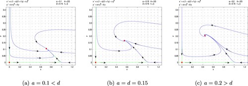However we note that both the predator and prey of system (6(6) $\begin{array}{rl}{x}^{\prime }& =\frac{x(1-x)}{1+fy}-xy\triangleq P_1(x,y),\\ y^{\prime }& =axy-dy\triangleq Q_1(x,y).\end{array}$(6) ) are globally stable only when a>d, and when $a\le d$ the predator is extinct. Hence the introduction of the mutual interference constant strengthens the stability of the system. Figure 7(a) –(c) show the global asymptotic stability of system (7(7) $\begin{array}{rl}{x}^{\prime }& =\frac{x(1-x)}{1+fy}-x{y}^{{\theta }_1}\triangleq P_2(x,y),\\ y^{\prime }& =ax{y}^{{\theta }_1}-dy\triangleq Q_2(x,y),\end{array}$(7) ) when ${\theta }_1=\frac{2}{3}$ under the assumptions a<d, a = d and a>d respectively.

Figure 7. Fear effect and mutual interference predator-prey model (7(7) $\begin{array}{rl}{x}^{\prime }& =\frac{x(1-x)}{1+fy}-x{y}^{{\theta }_1}\triangleq P_2(x,y),\\ y^{\prime }& =ax{y}^{{\theta }_1}-dy\triangleq Q_2(x,y),\end{array}$(7) ) with $f=3,d=0.15,{\theta }_1=\frac{2}{3}$. (a) a = 0.1<d, (b) a = d = 0.15 and (c) a = 0.2>d.

Incorporating system (6(6) $\begin{array}{rl}{x}^{\prime }& =\frac{x(1-x)}{1+fy}-xy\triangleq P_1(x,y),\\ y^{\prime }& =axy-dy\triangleq Q_1(x,y).\end{array}$(6) ) with group defense, the stability property of system (8(8) $\begin{array}{rl}{x}^{\prime }& =\frac{x(1-x)}{1+fy}-x^{{\theta }_2}y,\\ y^{\prime }& =a{x}^{{\theta }_2}y-dy,\end{array}$(8) ) is significantly different from that of systems (6(6) $\begin{array}{rl}{x}^{\prime }& =\frac{x(1-x)}{1+fy}-xy\triangleq P_1(x,y),\\ y^{\prime }& =axy-dy\triangleq Q_1(x,y).\end{array}$(6) ) and (7(7) $\begin{array}{rl}{x}^{\prime }& =\frac{x(1-x)}{1+fy}-x{y}^{{\theta }_1}\triangleq P_2(x,y),\\ y^{\prime }& =ax{y}^{{\theta }_1}-dy\triangleq Q_2(x,y),\end{array}$(7) ). It follows from Theorem 4.1 that there exists a separatrix curve such that the first quadrant is divided into two parts. In one part, from Theorem 4.1, the orbits will tend to the origin. In the other part, it follows from Theorems 4.2 and 4.3 that the orbits maybe tend to the boundary equilibria $E_1^3$ (Figures 8 a–b), the positive equilibrium $E_3^{\ast }$ (Figure 8 c), or the limit cycle (Figure 8 d). Note that the stability of boundary equilibria or positive equilibrium of systems (6(6) $\begin{array}{rl}{x}^{\prime }& =\frac{x(1-x)}{1+fy}-xy\triangleq P_1(x,y),\\ y^{\prime }& =axy-dy\triangleq Q_1(x,y).\end{array}$(6) ) and (7(7) $\begin{array}{rl}{x}^{\prime }& =\frac{x(1-x)}{1+fy}-x{y}^{{\theta }_1}\triangleq P_2(x,y),\\ y^{\prime }& =ax{y}^{{\theta }_1}-dy\triangleq Q_2(x,y),\end{array}$(7) ) is global. However, when considering system (6(6) $\begin{array}{rl}{x}^{\prime }& =\frac{x(1-x)}{1+fy}-xy\triangleq P_1(x,y),\\ y^{\prime }& =axy-dy\triangleq Q_1(x,y).\end{array}$(6) ) with group defense, the stability of boundary equilibria or positive equilibrium of system (8(8) $\begin{array}{rl}{x}^{\prime }& =\frac{x(1-x)}{1+fy}-x^{{\theta }_2}y,\\ y^{\prime }& =a{x}^{{\theta }_2}y-dy,\end{array}$(8) ) is just local due to the singularity of the origin. Considering the original coefficients of system (5(5) $\begin{array}{rl}{x}^{\prime }& =rx(1-\frac{x}{K})\frac{1}{1+fy}-pxy,\\ y^{\prime }& =hpxy-ey,\end{array}$(5) ), $a<d^{\ast }$ is equivalent to $K\le \frac{e}{hp}(\frac{2-{\theta }_2}{1-{\theta }_2}{)}^{{\theta }_2}$. Let the initial condition of system (8(8) $\begin{array}{rl}{x}^{\prime }& =\frac{x(1-x)}{1+fy}-x^{{\theta }_2}y,\\ y^{\prime }& =a{x}^{{\theta }_2}y-dy,\end{array}$(8) ) below the separatrix curve L. From Figure 9, if the carrying capacity K of prey is small enough (i.e. $K\le \frac{e}{hp}$), predator will be extinct, while prey will survive (see Figures 8 a,b). If the carrying capacity K of prey is an appropriate value (i.e. $\frac{e}{hp}<K<\frac{e}{hp}(\frac{2-{\theta }_2}{1-{\theta }_2}{)}^{{\theta }_2}$), predator and prey can coexist (see Figure 8 c). If the carrying capacity K of prey is large enough (i.e. $K>\frac{e}{hp}(\frac{2-{\theta }_2}{1-{\theta }_2}{)}^{{\theta }_2}$), predator and prey will oscillate periodically or be extinct (see Figures 8 d,e). System (8(8) $\begin{array}{rl}{x}^{\prime }& =\frac{x(1-x)}{1+fy}-x^{{\theta }_2}y,\\ y^{\prime }& =a{x}^{{\theta }_2}y-dy,\end{array}$(8) ) undergoes a supercritical Hopf bifurcation at positive equilibrium $E_3^{\ast }$ and exists a stable limit cycle around $E_3^{\ast }$. Compared with the global asymptotic stability of the positive equilibrium of system (6(6) $\begin{array}{rl}{x}^{\prime }& =\frac{x(1-x)}{1+fy}-xy\triangleq P_1(x,y),\\ y^{\prime }& =axy-dy\triangleq Q_1(x,y).\end{array}$(6) ) with a>d, when considering system (6(6) $\begin{array}{rl}{x}^{\prime }& =\frac{x(1-x)}{1+fy}-xy\triangleq P_1(x,y),\\ y^{\prime }& =axy-dy\triangleq Q_1(x,y).\end{array}$(6) ) with the group defense, by numerical simulation, we find that the limit cycle of system (8(8) $\begin{array}{rl}{x}^{\prime }& =\frac{x(1-x)}{1+fy}-x^{{\theta }_2}y,\\ y^{\prime }& =a{x}^{{\theta }_2}y-dy,\end{array}$(8) ) disappears when a is large enough, and the origin is globally stable, that is both prey and predator will be extinct (Figure 8 e), which means that the group defense can destabilize the system. Hence, the group defense makes the dynamics behaviour of system (8(8) $\begin{array}{rl}{x}^{\prime }& =\frac{x(1-x)}{1+fy}-x^{{\theta }_2}y,\\ y^{\prime }& =a{x}^{{\theta }_2}y-dy,\end{array}$(8) ) become more complicated.

Figure 8. Fear effect and group defense predator-prey model (8(8) $\begin{array}{rl}{x}^{\prime }& =\frac{x(1-x)}{1+fy}-x^{{\theta }_2}y,\\ y^{\prime }& =a{x}^{{\theta }_2}y-dy,\end{array}$(8) ) with $f=3,d=0.15,{\theta }_2=\frac{2}{3}$. (a) a = 0.1<d, (b) a = d = 0.15, (c) $d<a=0.2<d^{\ast }$, (d) $a=0.39>d^{\ast }$ and (e)$a=0.48>d^{\ast }$.

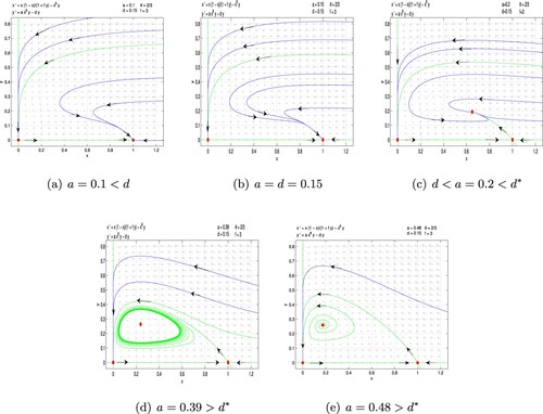
Figure 9. Bifurcation diagrams of system (8(8) $\begin{array}{rl}{x}^{\prime }& =\frac{x(1-x)}{1+fy}-x^{{\theta }_2}y,\\ y^{\prime }& =a{x}^{{\theta }_2}y-dy,\end{array}$(8) ). In region $D_2$, $E_1^{\ast }$ is unstable. In region $D_1$, $E_1^{\ast }$ is locally asymptotically stable. In region $D_0$, $E_1^1$ is locally asymptotically stable.

Disclosure statement

No potential conflict of interest was reported by the author(s).

Additional information

Funding

This work was supported by the Natural Science Foundation of Fujian Province (2021J01613, 2021J011032).

References

- V. Ajraldi, M. Pittavino, and E. Venturino, Modeling herd behavior in population systems, Nonlinear Anal. Real World Appl 12 (2011), pp. 2319–2338.
- Y. An and X. Luo, Global stability of a stochastic Lotka–Volterra cooperative system with two feedback controls, J. Nonlinear Model. Anal 2 (2020), pp. 131–142.
- R. Arditi, J. Callois, Y. Tyutyunov, and C. Jost, Does mutual interference always stabilize predator-prey dynamics? A comparison of models, C. R. Biologies 327 (2004), pp. 1037–1057.
- P. Braza, Predator-prey dynamics with square root functional responses, Nonlinear Anal. Real World Appl 13 (2012), pp. 1837–1843.
- P. Cong, M. Fan, and X. Zou, Dynamics of a three-species food chain model with fear effect, Commun. Nonlinear Sci. Numer. Simulat 99 (2021), pp. Article ID 105809.
- Y. Dai, Y. Zhao, and B. Sang, Four limit cycles in a predator-prey system of Leslie type with generalized Holling type III functional response, Nonlinear Anal. Real World Appl 50 (2019), pp. 218–239.
- W. Ding and W. Huang, Global dynamics of a ratio-dependent Holling–Tanner predator-prey system, J. Math. Anal. Appl 460 (2018), pp. 458–475.
- S. Djilali, Impact of prey herd shape on the predator-prey interaction, Chaos Solitons Fractals 120 (2019), pp. 139–148.
- H. Freedman, Stability analysis of a predator-prey system with mutual interference and density-dependent death rates, Bull Math. Biol 41 (1979), pp. 67–78.
- M. Hassell, Density dependence in single-species population, J. Anim. Ecol 44 (1975), pp. 283–295.
- M. He, F. Chen, and Z. Li, Permanence and global attractivity of an impulsive delay logistic model, Appl. Math. Lett 62 (2016), pp. 92–100.
- M. He and F. Chen, Extinction and stability of an impulsive system with pure delays, Appl. Math. Lett 91 (2019), pp. 128–136.
- M. Lu, J. Huang, S. Ruan, and P. Yu, Bifurcation analysis of an SIRS epidemic model with a generalized nonmonotone and saturated incidence rate, J. Differential Equations 267 (2019), pp. 1859–1898.
- S. Pal, N. Pal, S. Samanta, and J. Chattopadhyay, Effect of hunting cooperation and fear in a predator-prey model, Ecol. Complex 39 (2019), pp. Article ID 100770.
- L. Perko, Differential Equations and Dynamical Systems. third ed. Vol. 7, in: Texts in Applied Mathematics, Springer Verlag; New York: 2001
- T. Qiao, Y. Cai, S. Fu, and W. Wang, Stability and Hopf bifurcation in a predator-prey model with the cost of anti-predator behaviors, Int. J. Bifur. Chaos 29 (2019), pp. Article ID 1950185.
- S. Salman, A. Yousef, and A. Elsadany, Stability, bifurcation analysis and chaos control of a discrete predator-prey system with square root functional response, Chaos Solitons Fractals 93 (2016), pp. 20–31.
- S. Sasmal, Population dynamics with multiple allee effects induced by fear factors-A mathematical study on prey-predator interactions, Appl. Math. Model 64 (2018), pp. 1–14.
- Y. Song, H. Jiang, and Y. Yuan, Turing–Hopf bifurcation in the reaction-diffusion system with delay and application to a diffusive predator-prey model, J. Appl. Anal. Comput 9 (2019), pp. 1132–1164.
- Y. Song and T. Zhang, Spatial pattern formations in diffusive predator-prey systems with non-homogeneous Dirichlet boundary conditions, J. Appl. Anal. Comput 10 (2020), pp. 165–177.
- Y. Tan, Y. Cai, R. Yao, M. Hu, and W. Wang, Complex dynamics in an eco-epidemiological model with the cost of anti-predator behaviors, Nonlinear Dyn 107 (2022), pp. 3127–3141.
- Y. Tian, M. Han, and F. Xu, Bifurcations of small limit cycles in liénard systems with cubic restoring terms, J. Differential Equations 267 (2019), pp. 1561–1580.
- V. Tiwari, J. Tripathi, S. Mishra, and R. Upadhyay, Modeling the fear effect and stability of non-equilibrium patterns in mutually interfering predator-prey systems, Appl. Math. Comput 371 (2020), pp. Article ID 124948.
- E. Venturino and S. Petrovskii, Spatiotemporal behavior of a prey-predator system with a group defense for prey, Ecol. Complex 14 (2013), pp. 37–47.
- X. Wang, L. Zanette, and X. Zou, Modelling the fear effect in predator-prey interactions, J. Math. Biol 73 (2016), pp. 1–38.
- X. Wang, Y. Tan, Y. Cai, and W. Wang, Impact of the fear effect on the stability and bifurcation of a Leslie–Gower predator-prey model, Int. J. Bifur. Chaos 30 (2020), pp. Article ID 2050210.
- C.H. Wang, S.L. Yuan, and H. Wang, Spatiotemporal patterns of a diffusive prey-predator model with spatial memory and pregnancy period in an intimidatory environment, J. Math. Biol 84 (2022), pp. 1–36.
- K. Wang and Y. Zhu, Periodic solutions, permanence and global attractivity of a delayed impulsive prey-predator system with mutual interference, Nonlinear Anal. Real World Appl 14 (2013), pp. 1044–1054.
- Y. Xia and S. Yuan, Survival analysis of a stochastic predator-prey model with prey refuge and fear effect, J. Biol. Dynam 14 (2020), pp. 871–892.
- C. Xiang, J. Huang, S. Ruan, and D. Xiao, Bifurcation analysis in a host-generalist parasitoid model with Holling II functional response, J. Differential Equations 268 (2020), pp. 4618–4662.
- Z. Xiao and Z. Li, Stability analysis of a mutual interference predator-prey model with the fear effect, J. Appl. Sci. Eng 22 (2019), pp. 205–211.
- D. Xiao and S. Ruan, Global dynamics of a ratio-dependent predator–prey system, J. Math. Biol 43 (2001), pp. 68–290.
- C. Xu, S. Yuan, and T. Zhang, Global dynamics of a predator–prey model with defense mechanism for prey, Appl. Math. Lett 62 (2016), pp. 42–48.
- S. Yan, D. Jia, T. Zhang, and S. Yuan, Pattern dynamic in a diffusive predator-prey model with hunting cooperations, Chaos Solitons Fractals 130 (2020), pp. Article ID 109428.
- S. Yuan, D. Wu, G. Lan, and H. Wang, Noise-induced transitions in a nonsmooth predator-prey model with stoichiometric constraints, Bull. Math. Biol. 82 (2020), pp. 55.
- L. Zanette, A. White, M. Allen, and M. Clinchy, Perceived predation risk reduces the number of offspring songbirds produce per year, Science 334 (2011), pp. 1398–1401.
- H. Zhang, Y. Cai, S. Fu, and W. Wang, Impact of the fear effect in a prey-predator model incorporating a prey refuge, Appl. Math. Comput 356 (2019), pp. 328–337.
- X. Zhang, G. Huang, and Y. Dong, Dynamical analysis on a predator-prey model with stage structure and mutual interference, J. Biol. Dynam 14 (2020), pp. 200–221.
- Z. Zhang, T. Ding, W. Huang, and Z. Dong, Qualitative Theory of Differential Equations, Transl. Math. Monogr. vol. 101, Amer. Math. Soc., Providence, RI, 1992
- Z. Zhu, Y. Chen, Z. Li, and F. Chen, Stability and bifurcation in a Leslie–Gower predator-prey model with Allee effect, Int. J. Bifur. Chaos 32 (2022), pp. Article ID 2250040.