Modeling malaria transmission in Nepal: impact of imported cases through cross-border mobility

ABSTRACT

The cross-border mobility of malaria cases poses an obstacle to malaria elimination programmes in many countries, including Nepal. Here, we develop a novel mathematical model to study how the imported malaria cases through the Nepal-India open-border affect the Nepal government's goal of eliminating malaria by 2026. Mathematical analyses and numerical simulations of our model, validated by malaria case data from Nepal, indicate that eliminating malaria from Nepal is possible if strategies promoting the absence of cross-border mobility, complete protection of transmission abroad, or strict border screening and isolation are implemented. For each strategy, we establish the conditions for the elimination of malaria. We further use our model to identify the control strategies that can help maintain a low endemic level. Our results show that the ideal control strategies should be designed according to the average mosquito biting rates that may depend on the location and season.

KEYWORDS:

• Cross-border mobility
• malaria elimination programme
• imported malaria cases
• mathematical model
• Nepal

MATHEMATICS SUBJECT CLASSIFICATIONS 2010:

• 34D20
• 37N25
• 92B05
• 92C50

1. Introduction

Malaria continues to pose a global health burden and is one of the leading causes of death in many developing countries [11]. In 2019, about 229 million cases of malaria and 409 thousand malaria-related deaths were estimated worldwide, mainly in African countries [30,67]. Despite the continuous control efforts with programmes targeting elimination, malaria cases have slightly increased globally for the past few years. According to the WHO reports, the total number of worldwide malaria cases in 2016, 2017, 2018, 2019, and 2020 are 214, 217, 219, 228, and 229 million, respectively. In pursuit of malaria elimination, broad access to human mobility has been a primary obstacle to successful malaria control in many countries, including Nepal [23]. In particular, the human mobility between low and high endemic countries results in the importation of malaria cases from high to low endemic countries, causing potentiality for the resurgence of malaria in low endemic countries. Notably, the cross-border migrants contribute to the transfer of malaria cases from high to low endemic countries [33]. For example, even though the elimination of malaria from Spain was declared in 1964, about 10,000 cases were reported, mostly in travellers and migrants, in a later year. Similarly, about 12,000 to 15,000 cases of malaria are imported to European Union (EU) every year, with the majority to France, the UK, and Germany from West Africa [32,59,68]. Given the significant obstacle to malaria elimination due to human mobility across borders, studying the impact of the imported cases through cross-border mobility on the malaria elimination programmes is critical.

Nepal is one of the countries facing the direct consequence of a cross-border transfer of malaria cases due to its open border provision with India. Although the malaria elimination programmes in Nepal started in 1958 [25], the trend of malaria cases remained fluctuated between 1963 and 2018, with a peak in 1985 (more than 42,321 cases) [22,28]. After 1985, the number of cases steadily declined, and the transmission rate eventually reached a low level of 0.08 per 1000 annual parasite incidence (API) among the risk population in 2018 [66]. With this rapidly decreasing- trend, the Nepal government has set the goal of zero indigenous malaria by 2022 and malaria elimination by 2026 [29]. However, the porous border between Nepal and India has been a severe concern for achieving these goals because even though the number of total cases declined from 2009 (3500 cases) to 2018 (1065 cases) by 69%, the net imported cases increased during this period by approximately 40 to 58% [28]. Most of these imported cases reported a history of travel to malaria-endemic areas of India [29]. An increase in imported cases has posed an uncertainty about the elimination programmes to meet Nepal's goal set. Mathematical modelling can provide a valuable tool to predict the potential impact of such imported cases on malaria elimination from Nepal.

Since the first differential equation-based model introduced by Ronald Ross in 1911 [12], various mathematical models have been developed to study the impact of control and prevention policies on the incidence of malaria in many endemic regions [6,18,19,36,42,48,54]. These models have been further extended by incorporating age structure, loss of immunity, the effect of social, economic, and environmental factors, human migration, drug resistance of vector, the impact of bed-nets, multi-groups, and multi patches [2–4,7,10,16,20,31,37,45–47,52,61–63]. Even though some mathematical models [8,17,39,51,58] include cross-border mobility, there remains uncertainty on the various aspects of the role of imported cases in vector-borne disease, particularly malaria transmission. Except for some descriptive, analytical, and retrospective studies [21,25,55,57,66], none of the previous models focused on the dynamics of indigenous and imported malaria cases in the context of Nepal, which is in critical condition of achieving the 2026 malaria elimination goal due to cross-border mobility of migrant workers.

Motivated from a previous study [64], which addressed the impact of cross-border mobility on HIV-AIDS epidemics in Nepal, we develop a novel transmission dynamics model of malaria by incorporating the imported cases through the cross-border mobility into a basic malaria model. Using the data of malaria cases in Nepal, we estimate the critical parameters of malaria dynamics in Nepal. We thoroughly analyze our model to study the impact of cross-border mobility on disease eradication and threshold dynamics. We further use our model to predict the future trend of imported and indigenous malaria cases and evaluate the different control strategies to achieve the malaria elimination goal by 2026.

2. Mathematical model

2.1. Model formulation

To develop a transmission dynamics model of malaria, we divide the total population of the home country into two groups: the population living in the home country ($N_{hH}$) and the population living abroad as migrant workers $\left(N_{hM}\right)$. Each of these groups is further divided into three subgroups: susceptible $\left(S_{hH}\right)$, infectious $\left(I_{hH}\right)$, and recovered $\left(R_{hH}\right)$ in the home country and susceptible $\left(S_{hM}\right)$, infectious $\left(I_{hM}\right)$, and recovered $\left(R_{hM}\right)$ living abroad as migrant workers. Moreover, we consider susceptible and infectious mosquito populations in the home country ($S_{vH},I_{vH}$) and abroad ($S_{vA},I_{vA}$). We note that the migrant workers, $N_{hM}$, are included in the total human population abroad $\left(N_{hA}\right)$ and thus the corresponding abroad groups, susceptible $\left(S_{hA}\right)$, infectious $\left(I_{hA}\right)$, and recovered $\left(R_{hA}\right)$ include $S_{hM}$, $I_{hM}$, and $R_{hM}$, respectively.

In our model, malaria transmission occurs from infected mosquitoes to susceptible humans and from infected humans to susceptible mosquitoes through mosquito bites. We assume that b and $b^{\prime }$ are the per capita biting rates of mosquitoes in the home country and abroad, respectively. ${\alpha }_{vh}$ and ${\alpha }_{vh}^{\prime }$ are the probability in the home country and abroad, respectively, that an infectious mosquito transmit malaria to a susceptible human in a single bite. Similarly, ${\alpha }_{hv}$ and ${\alpha }_{hv}^{\prime }$ are the probability in the home country and abroad, respectively, that the malaria is transmitted from infectious human to a susceptible mosquito in a single infectious bite. For the home country, the total number of bites (per time) from all the infectious mosquitoes is $b{I}_{vH}$ (infectious bites). Among these bites, the susceptible humans get $\frac{b{I}_{vH}{S}_{hH}}{N_{hH}}$ infectious bites. Therefore, the incidence rate of humans (i.e. the new human infections per unit time) is $\frac{b{\alpha }_{vh}{I}_{vH}{S}_{hH}}{N_{hH}}$ [2,14,15,34,40,71,72]. Similarly, the incidence rate for humans in abroad is $\frac{b^{\prime }{\alpha }_{vh}^{\prime }{I}_{vA}{S}_{hA}}{N_{hA}}$. Also, the total number of bites (per time) made by the susceptible mosquitoes in the home country is $b{S}_{vH}$. Among these bites, the total number of bites from the infectious humans (infectious bites) is $\frac{b{S}_{vH}{I}_{hH}}{N_{hH}}$. Therefore, the Incidence rate of mosquitoes (i.e. the new mosquito infections per unit time) is $\frac{b{\alpha }_{hv}{I}_{hH}{S}_{vH}}{N_{hH}}$. Similarly, the incidence rates for mosquitoes in abroad is $\frac{b^{\prime }{\alpha }_{hv}^{\prime }{I}_{hA}{S}_{vA}}{N_{hA}}$.

The infectious humans recover with the rate ${\gamma }_h$, and the recovered individuals lose their immunity and move back to the susceptible class at the rate q. Because of the short lifespan of mosquitoes, we do not consider the recovered class for the mosquitoes population. The parameters Λ and $d_h$ represent the recruitment rate and the natural death rate of humans, respectively, while the parameters ϕ and $d_v$ represent the recruitment rate and the death rate of mosquitoes, respectively. We assume that η represents the per capita cross-border mobility rate for susceptible populations ($S_{hH},S_{hM}$) and recovered populations ($R_{hH},R_{hM}$). Since infected individuals may behave differently in their travels from and to the home country, we take p and θ as the cross-border mobility rate for infectious individuals from and to the home country, respectively. In the model, $\theta I_{hM}$ and $\frac{b{\alpha }_{vh}{I}_{vH}{S}_{hH}}{N_{hH}}$ represent the imported and indigenous malaria incidence at home country, respectively.

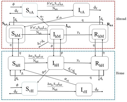
The schematic diagram of our model is presented in Figure 1. The system of equations describing the transmission dynamics of malaria discussed above is as follows: (1) $\begin{array}{rl}{S}_{hH}^{\prime }& =\mathrm{\Lambda }+\eta S_{hM}+q{R}_{hH}-\frac{b{\alpha }_{vh}{I}_{vH}}{N_{hH}}{S}_{hH}-(\eta +d_h)S_{hH},\end{array}$(1) (2) $\begin{array}{rl}{I}_{hH}^{\prime }& =\frac{b{\alpha }_{vh}{I}_{vH}}{N_{hH}}{S}_{hH}+\theta I_{hM}-(p+d_h+{\delta }_h+{\gamma }_h)I_{hH},\end{array}$(2) (3) $\begin{array}{rl}{R}_{hH}^{\prime }& ={\gamma }_h{I}_{hH}+\eta R_{hM}-(\eta +d_h+q)R_{hH},\end{array}$(3) (4) $\begin{array}{rl}{S}_{vH}^{\prime }& =\varphi -\frac{b{\alpha }_{hv}{I}_{hH}}{N_{hH}}{S}_{vH}-d_v{S}_{vH},\end{array}$(4) (5) $\begin{array}{rl}{I}_{vH}^{\prime }& =\frac{b{\alpha }_{hv}{I}_{hH}}{N_{hH}}{S}_{vH}-d_v{I}_{vH},\end{array}$(5) (6) $\begin{array}{rl}{S}_{hM}^{\prime }& =\eta S_{hH}+q{R}_{hM}-\frac{b^{\prime }{\alpha }_{vh}^{\prime }{I}_{vA}}{N_{hA}}{S}_{hM}-(d_h+\eta )S_{hM},\end{array}$(6) (7) $\begin{array}{rl}{I}_{hM}^{\prime }& =\frac{b^{\prime }{\alpha }_{vh}^{\prime }{I}_{vA}}{N_{hA}}{S}_{hM}+p{I}_{hH}-(\theta +{\delta }_h+d_h+{\gamma }_h)I_{hM},\end{array}$(7) (8) $\begin{array}{rl}{R}_{hM}^{\prime }& ={\gamma }_h{I}_{hM}+\eta R_{hH}-(\eta +d_h+q)R_{hM},\end{array}$(8) (9) $\begin{array}{rl}{S}_{vA}^{\prime }& =\varphi -\frac{b^{\prime }{\alpha }_{hv}^{\prime }{I}_{hA}}{N_{hA}}{S}_{vA}-d_v{S}_{vA},\end{array}$(9) (10) $\begin{array}{rl}{I}_{vA}^{\prime }& =\frac{b^{\prime }{\alpha }_{hv}^{\prime }{I}_{hA}}{N_{hA}}{S}_{vA}-d_v{I}_{vA}.\end{array}$(10)

Figure 1. Malaria transmission dynamics with cross-border mobility. The upper SI-SIRS (inside red dashed line) and lower SI-SIRS (inside blue dashed line) represent the dynamics of malaria abroad and in the home country. The solid arrows represent the transfer of populations, and the dotted arrows represent the interaction between the susceptible human and infectious female Anopheles mosquitoes and infectious humans with susceptible female Anopheles mosquitoes. Here, subscripts H, A, and M refer to home, abroad, and migrant, respectively, and the subscript h and v refer to human and vector (mosquito), respectively.

2.2. Approximation to incidence rate abroad

Since the detailed dynamics of malaria abroad makes the model extremely complex and uncertain, we introduce an index $\psi \left(t\right)$ called Annual Parasite Incidence (API), for which the data are publicly available. We introduce this index into the model to approximate the incidence rate abroad. Here $\psi \left(t\right)$ is defined as the number of positive cases of malaria per population under surveillance, i.e. $\psi \left(t\right)=\frac{I_{hA}\left(t\right)}{N_{hA}\left(t\right)}$. The incidence rate of humans in abroad is given by ${\lambda }_h^{\prime }=\frac{b^{\prime }{\alpha }_{vh}^{\prime }{I}_{vA}\left(t\right)}{N_{hA}\left(t\right)}=\frac{b^{\prime }{\alpha }_{vh}^{\prime }{I}_{vA}\left(t\right)}{I_{hA}\left(t\right)}\psi \left(t\right).$Both $b^{\prime }{\alpha }_{vh}^{\prime }{I}_{vA}\left(t\right)$ and $I_{hA}\left(t\right)$ are differentiable functions in the interval $[0,T]$, where T is the final time of the disease dynamics considered. Assuming that $I_{hA}\left(t\right)\ne 0,\mathrm{\forall }t\in [0,T]$, the mean value theorem of integral calculus allows us to approximate the integral of the continuous function $\frac{b^{\prime }{\alpha }_{vh}^{\prime }{I}_{vA}\left(t\right)}{I_{hA}\left(t\right)}$ with a constant $\zeta =\frac{b^{\prime }{\alpha }_{vh}^{\prime }}{T}{\int }_0^T\frac{I_{vA}\left(t\right)}{I_{hA}\left(t\right)}\mathrm{d}t\approx b^{\prime }{\alpha }_{vh}^{\prime }\frac{I_{vA}\left(t_0\right)}{I_{hA}\left(t_0\right)}$ for some $t_0\in (0,T)$. Thus, we approximate the incidence rate abroad by ${\lambda }_h^{\prime }=\zeta \psi \left(t\right)$ and estimate the value of ζ from the data fitting. With this approximation, the system (1(1) $\begin{array}{rl}{S}_{hH}^{\prime }& =\mathrm{\Lambda }+\eta S_{hM}+q{R}_{hH}-\frac{b{\alpha }_{vh}{I}_{vH}}{N_{hH}}{S}_{hH}-(\eta +d_h)S_{hH},\end{array}$(1) )–(10(10) $\begin{array}{rl}{I}_{vA}^{\prime }& =\frac{b^{\prime }{\alpha }_{hv}^{\prime }{I}_{hA}}{N_{hA}}{S}_{vA}-d_v{I}_{vA}.\end{array}$(10) ) reduces to the system of the following eight differential equations. (11) $\begin{array}{rl}{S}_{hH}^{\prime }& =\mathrm{\Lambda }+\eta S_{hM}+q{R}_{hH}-\frac{b{\alpha }_{vh}{I}_{vH}}{N_{hH}}{S}_{hH}-(\eta +d_h)S_{hH},\end{array}$(11) (12) $\begin{array}{rl}{I}_{hH}^{\prime }& =\frac{b{\alpha }_{vh}{I}_{vH}}{N_{hH}}{S}_{hH}+\theta I_{hM}-(p+d_h+{\delta }_h+{\gamma }_h)I_{hH},\end{array}$(12) (13) $\begin{array}{rl}{R}_{hH}^{\prime }& ={\gamma }_h{I}_{hH}+\eta R_{hM}-(\eta +d_h+q)R_{hH},\end{array}$(13) (14) $\begin{array}{rl}{S}_{vH}^{\prime }& =\varphi -\frac{b{\alpha }_{hv}{I}_{hH}}{N_{hH}}{S}_{vH}-d_v{S}_{vH},\end{array}$(14) (15) $\begin{array}{rl}{I}_{vH}^{\prime }& =\frac{b{\alpha }_{hv}{I}_{hH}}{N_{hH}}{S}_{vH}-d_v{I}_{vH},\end{array}$(15) (16) $\begin{array}{rl}{S}_{hM}^{\prime }& =\eta S_{hH}+q{R}_{hM}-\zeta \psi \left(t\right)S_{hM}-(d_h+\eta )S_{hM},\end{array}$(16) (17) $\begin{array}{rl}{I}_{hM}^{\prime }& =\zeta \psi \left(t\right)S_{hM}+p{I}_{hH}-(\theta +{\delta }_h+d_h+{\gamma }_h)I_{hM},\end{array}$(17) (18) $\begin{array}{rl}{R}_{hM}^{\prime }& ={\gamma }_h{I}_{hM}+\eta R_{hH}-(\eta +d_h+q)R_{hM}.\end{array}$(18)

3. Parameters and model validation

3.1. Data

In this study, we used the data containing both indigenous and imported malaria cases in Nepal. Since the total cases were not classified as imported and indigenous before 2009, we considered the data only from 2009 to 2019 for our model fitting. The primary data sources related to malaria cases in Nepal are the National Malaria Surveillance Guidelines 2019 published by the Government of Nepal, Ministry of Health and Population Department of Health Services Epidemiology and Disease Control Division (EDCD) [21,28]. In addition, we also obtained the data of Annual Parasitic Incidence (API) of India from the Malaria Site India [41,44].

3.2. Parameter estimation

The population of Nepal was estimated to be 23,151,423 in 2001 [69] and 26,494,504 in 2011 [70]. Taking the average population growth per year from 2001 to 2011, we estimated the population of Nepal in 2009 (the base year of our dynamics, i.e. t = 0) to be 25,825,888. About 5.5 million Nepalese, including 1.9 million male workers, were living abroad [38], mostly in India. These migrant workers bring malaria upon their return home, contributing the significant number of imported malaria cases in Nepal [29]. Note that the majority of Nepalese migrants working in India are male [64]. Therefore, we took $N_{hM}\left(0\right)=1.9$ million. With 5.5 million living abroad, the population inside Nepal is approximately 20,325,888. Since most of the hilly and mountainous regions of Nepal are considered risk free zone of malaria, leaving only about 48% of Nepalese residing in other regions in high, moderate or low risk area [50], we estimated $N_{hH}\left(0\right)=\mathrm{9,756,426}$. Moreover, we used the information from the data and divided the total population into different compartments and obtained $S_{hH}\left(0\right)=\mathrm{9,754,000},I_{hH}\left(0\right)=2000,R_{hH}\left(0\right)=426,S_{hM}\left(0\right)=\mathrm{1,898,300},I_{hM}\left(0\right)=1400,R_{hM}\left(0\right)=300,S_{vH}\left(0\right)=\mathrm{9,754,176}$, and $I_{vH}\left(0\right)=2250$. About 37.5% of the total migrant workers ($\sim \mathrm{179,464}$) travelled from Nepal to India in 2009 [27]. This allows us to estimate per capita annual mobility rate of migrants from Nepal to India as $\eta =\frac{\mathrm{N}\mathrm{u}\mathrm{m}\mathrm{b}\mathrm{e}\mathrm{r}\mathrm{o}\mathrm{f}\mathrm{m}\mathrm{i}\mathrm{g}\mathrm{r}\mathrm{a}\mathrm{n}\mathrm{t}\mathrm{s}\mathrm{f}\mathrm{r}\mathrm{o}\mathrm{m}\mathrm{N}\mathrm{e}\mathrm{p}\mathrm{a}\mathrm{l}\mathrm{t}\mathrm{o}\mathrm{I}\mathrm{n}\mathrm{d}\mathrm{i}\mathrm{a}}{\mathrm{T}\mathrm{o}\mathrm{t}\mathrm{a}\mathrm{l}\mathrm{r}\mathrm{i}\mathrm{s}\mathrm{k}\mathrm{p}\mathrm{o}\mathrm{p}\mathrm{u}\mathrm{l}\mathrm{a}\mathrm{t}\mathrm{i}\mathrm{o}\mathrm{n}\mathrm{o}\mathrm{f}\mathrm{m}\mathrm{a}\mathrm{l}\mathrm{a}\mathrm{r}\mathrm{i}\mathrm{a}\mathrm{i}\mathrm{n}\mathrm{N}\mathrm{e}\mathrm{p}\mathrm{a}\mathrm{l}}=\frac{179,464}{9,756,426}=0.0183\left(\mathrm{p}\mathrm{e}\mathrm{r}\mathrm{h}\mathrm{u}\mathrm{m}\mathrm{a}\mathrm{n}\mathrm{p}\mathrm{e}\mathrm{r}\mathrm{y}\mathrm{e}\mathrm{a}\mathrm{r}\right)$.

The Crude Birth Rate (CBR), i.e. the number of live birth per year per 1000 people, of Nepal for the year 2009 was 23.189 [70], which implies the human recruitment rate per year for the population in the risk area is $\mathrm{\Lambda }=48\mathrm{\%}\text{of}\frac{23.189\times \mathrm{25,825,888}}{1000}=\mathrm{287,460}$. Since the average life expectancy of Nepalese individuals in 2009 was 67.178 years [60], the natural death rate of humans per year is taken as $d_h=0.0149$ per year. The number of deaths due to malaria in the base year [26] was 6, so we calculated ${\delta }_h=0.0017$ per year. The duration of immunity for recovered people varies widely from region to region, and we took the immunity period to be 3 months, i.e. q = 4 per year [15]. For model fitting, we assumed that all the cases are recorded and that malaria-infected Nepalese do not move to India as workers while sick. Therefore, we took p=0.

The population of female Anopheles mosquitoes has been estimated to be 1–10 times the human population [13,15,34]. Thus we took the mosquito population equal to base year human population 9,756,426. Based on the previous studies [1,9,13,15,34], we took the probability of disease transmission, per bite, from an infectious mosquito to a susceptible human as ${\alpha }_{vh}=0.0195$, and from an infectious human to a susceptible mosquito as ${\alpha }_{hv}=0.63$. Similarly, the human recovery rate and the mosquito death rate were obtained from previous studies as ${\gamma }_h=1.85$ per year and $d_v=27.9113$ per year [1,9,13,15,34]. The remaining parameters, θ, ζ, and b, were estimated from the data fitting.

3.3. Model fitting to the data

As per the national planning of malaria elimination by 2026, the Government of Nepal introduced the strategic plan in 2014, which includes the distribution of Long Lasting Insecticide Treated Nets (LLINs) and Indoor Residual Spraying (IRS) intended to reduce mosquito bites [29]. Thus in our model fitting, we allow the different biting rates for the period before ($b=b_1$) and after ($b=b_2$) 2014.

The available data are the yearly indigenous malaria incidence, the yearly imported malaria incidence, and the total malaria incidence in Nepal. From the solution of our model, the indigenous, the imported, and the total malaria incidences at time t, denoted by $L\left(t\right)$, $I\left(t\right)$, and $T\left(t\right)$, respectively, can be computed using the following expressions: (19) $L\left(t\right)=\frac{b{\alpha }_{vh}{S}_{hH}{I}_{vH}}{N_{hH}},I\left(t\right)=\theta I_{hM},T\left(t\right)=\frac{b{\alpha }_{vh}{S}_{hH}{I}_{vH}}{N_{hH}}+\theta I_{hM}.$(19) The model system of differential equations was solved numerically using the fourth-order Runge-Kutta method. Using the solutions, we obtained the best-fit parameters using the nonlinear least-squares regression method that minimizes the following sum of the squared residuals: (20) $J\left(\varphi \right)=\sum _{k=1}^n\left[\right(L\left(t_k\right)-\overline{L}\left(t_k\right){)}^2+\left(I\right(t_k)-\overline{I}(t_k){)}^2+(T\left(t_k\right)-\overline{T}\left(t_k\right){)}^2],$(20) where $L\left(t_k\right),I\left(t_k\right),T\left(t_k\right)$ and $\overline{L}\left(t_k\right),\overline{I}\left(t_k\right),\overline{T}\left(t_k\right)$ are the model predicted incidences and those given in the available data. In our data fitting, we used the total 30 data points to estimate four parameters $\mathrm{\Phi }=(\theta ,\zeta ,b_1,b_2)$. The ratio of data to the free parameters used in our model, i.e. 7:1, is well within the recommended range of 5:1–10:1 [53]. Also, three types of data (indigenous, imported, and total) included in fitting provide additional feature of malaria infection. To obtain the confidence limits for the estimated parameters, we computed standard errors from the sensitivity matrix S using the techniques described previously [49]. Furthermore, we computed the rank of the matrix $S^{T}S$ and found the matrix to be of the full rank (rank $=4$), which ascertain the identifiability of these parameters of the model [43]. All computations were carried out in MATLAB (The MathWorks, Inc.).

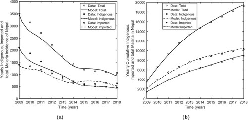
In Figure 2, we present the model prediction, along with the data, of the indigenous, the imported, and the total malaria incidence. The model fits have captured the dynamics pattern of the multiple data well, and the model prediction is also consistent with the cumulative data (Figure 2), thereby validating the model. All estimated parameters, as well as the fixed parameters, are provided in Table 2. As indicated by the data [29], the model solutions also show the decreasing trend of the malaria cases from 2009, with the indigenous case being more than the imported case until 2014. However, after 2014, the imported case overtook the indigenous case, indicating the alarming situation originating from the imported cases.

Figure 2. Model fitting to the data. (a) Solution of the fitted model along with the data of indigenous, imported, and total malaria incidences in Nepal, and (b) Model prediction of cumulative indigenous, cumulative imported, and cumulative total cases in Nepal.

Our estimates show that the biting rate of mosquitoes is $b_1=48.0$ (95% CI: [38.13, 57.87]) before 2014, and $b_2=39.5$ (95% CI: [29.63, 49.37]) after 2014. These estimated values are consistent with the values provided in many previous studies [15,34]. Similarly, we estimated the disease import rate $\theta =0.98$ (95% CI: [0.42, 1.54]) and the parameter corresponding to the incidence rate in India $\zeta =0.00105$ (95% CI: [0.0005, 0.0016]).

4. Model analysis

Note that our model is non-autonomous due to the presence of time-dependent parameter $\psi \left(t\right)$. Since $\psi \left(t\right)$ depends on the policy implemented abroad, the time-dependent nature of this parameter remains unknown, and the analysis of this non-autonomous model is complicated and uncertain. Therefore, for the purpose of analysis, we consider the autonomous form of the model by taking a constant $k=\left(\zeta /T\right){\int }_0^T\psi \left(t\right)\mathrm{d}t$ as an approximation to the incidence rate abroad.

4.1. Basic properties of model: positivity and boundedness

In this section, we show that the solutions of all the state variables are non-negative and bounded in order to demonstrate that the model is well-posed and biologically valid for describing malaria transmission dynamics. The results are presented in the following theorem.

Theorem 4.1

If $S_{hH}\left(0\right)>0,I_{hH}\left(0\right)\ge 0,R_{hH}\left(0\right)\ge 0,S_{hM}\left(0\right)\ge 0,I_{hM}\left(0\right)\ge 0,R_{hM}\left(0\right)\ge 0,S_{vH}\left(0\right)>0,I_{vH}\left(0\right)\ge 0$, then the solution set $\left\{S_{hH}\right(t),I_{hH}(t),R_{hH}(t),S_{hM}(t),I_{hM}(t),R_{hM}(t),S_{vH}(t),I_{vH}(t\left)\right\}$ of the system (11(11) $\begin{array}{rl}{S}_{hH}^{\prime }& =\mathrm{\Lambda }+\eta S_{hM}+q{R}_{hH}-\frac{b{\alpha }_{vh}{I}_{vH}}{N_{hH}}{S}_{hH}-(\eta +d_h)S_{hH},\end{array}$(11) )–(18(18) $\begin{array}{rl}{R}_{hM}^{\prime }& ={\gamma }_h{I}_{hM}+\eta R_{hH}-(\eta +d_h+q)R_{hM}.\end{array}$(18) ) is always non-negative and bounded.

Proof.

See Appendix A.1.

Using the above conditions, we derive that for any $ϵ>0$, there exists $t_{ϵ}>0$ such that the solution of the system with $t\ge t_{ϵ}$ lies in the compact set $\mathrm{\Omega }={\mathrm{\Omega }}_h\times {\mathrm{\Omega }}_v$, where ${\mathrm{\Omega }}_h=\left\{\right(S_{hH},I_{hH},R_{hH},S_{hM},I_{hM},R_{hM})\in {\mathrm{\Re }}_{+}^6:N_h\le \frac{\mathrm{\Lambda }}{d_h}+ϵ\}$and ${\mathrm{\Omega }}_v=\left\{\right(S_{vH},I_{vH})\in {\mathrm{\Re }}_{+}^2:N_v\le \frac{\varphi }{d_v}+ϵ\}.$

4.2. Existence of equilibria

For convenience, we let $S_{hH}=x,I_{hH}=y,R_{hH}=z,S_{hM}=X,I_{hM}=Y,R_{hM}=Z,S_{vH}=l$, and $I_{vH}=m$, and we take $(x^{\ast },y^{\ast },z^{\ast },l^{\ast },m^{\ast },X^{\ast },Y^{\ast },Z^{\ast })$ to represent the equilibrium point of the system (11(11) $\begin{array}{rl}{S}_{hH}^{\prime }& =\mathrm{\Lambda }+\eta S_{hM}+q{R}_{hH}-\frac{b{\alpha }_{vh}{I}_{vH}}{N_{hH}}{S}_{hH}-(\eta +d_h)S_{hH},\end{array}$(11) )–(18(18) $\begin{array}{rl}{R}_{hM}^{\prime }& ={\gamma }_h{I}_{hM}+\eta R_{hH}-(\eta +d_h+q)R_{hM}.\end{array}$(18) ). For simplicity, we assume that also for the infectious compartments, the mobility rate is equal in both ways, from home to abroad and vice versa, i.e. $\theta =p$. Taking, (21) ${\lambda }_h^{\ast }={\text{β}}_h\frac{m^{\ast }}{N_{hH}^{\ast }},{\lambda }_v^{\ast }={\text{β}}_v\frac{y^{\ast }}{N_{hH}^{\ast }},{\text{β}}_v=b{\alpha }_{hv},{\text{β}}_h=b{\alpha }_{vh},$(21) the system (11(11) $\begin{array}{rl}{S}_{hH}^{\prime }& =\mathrm{\Lambda }+\eta S_{hM}+q{R}_{hH}-\frac{b{\alpha }_{vh}{I}_{vH}}{N_{hH}}{S}_{hH}-(\eta +d_h)S_{hH},\end{array}$(11) )–(18(18) $\begin{array}{rl}{R}_{hM}^{\prime }& ={\gamma }_h{I}_{hM}+\eta R_{hH}-(\eta +d_h+q)R_{hM}.\end{array}$(18) ) provides (22) $\begin{array}{rl}& x^{\ast }=\frac{P}{K_1+K_2{\lambda }_h^{\ast }},y^{\ast }=\frac{Q_1+Q_2{\lambda }_h^{\ast }}{K_1+K_2{\lambda }_h^{\ast }},z^{\ast }=\frac{Q_3+Q_4{\lambda }_h^{\ast }}{K_1+K_2{\lambda }_h^{\ast }},\\ & X^{\ast }=\frac{S_1+S_2{\lambda }_h^{\ast }}{K_1+K_2{\lambda }_h^{\ast }},Y^{\ast }=\frac{T_1+T_2{\lambda }_h^{\ast }}{K_1+K_2{\lambda }_h^{\ast }},Z^{\ast }=\frac{U_1+U_2{\lambda }_h^{\ast }}{K_1+K_2{\lambda }_h^{\ast }},\end{array}$(22) where $P,Q_1,Q_2,Q_3,Q_4,S_1,S_2,T_1,T_2,U_1,U_2,K_1,K_2$ are non-negative constants with the combination of model parameters computed using Wolfram Mathematica. The closed-forms of these expressions are provided in Supplementary Material A (page 1–3). With some algebraic manipulation, we obtain (23) $\begin{array}{rl}& N_{hH}^{\ast }=\frac{P+Q_1+Q_3+{\lambda }_h^{\ast }(Q_2+Q_4)}{K_1+K_2{\lambda }_h^{\ast }},{\lambda }_v^{\ast }=\frac{{\text{β}}_v(Q_1+Q_2{\lambda }_h^{\ast })}{P+Q_1+Q_3+{\lambda }_h^{\ast }(Q_2+Q_4)},\\ & m^{\ast }=\frac{\varphi {\text{β}}_v(Q_1+Q_2{\lambda }_h^{\ast })}{d_v({\text{β}}_v{Q}_1+d_{v}P+Q_1{d}_v+Q_3{d}_v+(Q_2{d}_v+Q_4{d}_v+{\text{β}}_v{Q}_2\left){\lambda }_h^{\ast }\right)},l^{\ast }=\frac{\varphi -m^{\ast }{d}_v}{d_v}.\end{array}$(23) Then, from (21(21) ${\lambda }_h^{\ast }={\text{β}}_h\frac{m^{\ast }}{N_{hH}^{\ast }},{\lambda }_v^{\ast }={\text{β}}_v\frac{y^{\ast }}{N_{hH}^{\ast }},{\text{β}}_v=b{\alpha }_{hv},{\text{β}}_h=b{\alpha }_{vh},$(21) ) and (23(23) $\begin{array}{rl}& N_{hH}^{\ast }=\frac{P+Q_1+Q_3+{\lambda }_h^{\ast }(Q_2+Q_4)}{K_1+K_2{\lambda }_h^{\ast }},{\lambda }_v^{\ast }=\frac{{\text{β}}_v(Q_1+Q_2{\lambda }_h^{\ast })}{P+Q_1+Q_3+{\lambda }_h^{\ast }(Q_2+Q_4)},\\ & m^{\ast }=\frac{\varphi {\text{β}}_v(Q_1+Q_2{\lambda }_h^{\ast })}{d_v({\text{β}}_v{Q}_1+d_{v}P+Q_1{d}_v+Q_3{d}_v+(Q_2{d}_v+Q_4{d}_v+{\text{β}}_v{Q}_2\left){\lambda }_h^{\ast }\right)},l^{\ast }=\frac{\varphi -m^{\ast }{d}_v}{d_v}.\end{array}$(23) ), we obtain (24) $a_0{\lambda }_h^{\ast 3}+a_1{\lambda }_h^{\ast 2}+a_2{\lambda }_h^{\ast }+a_3=0,$(24) where, $\begin{array}{rl}{a}_0& =Q_2{Q}_4{d}_v{\text{β}}_v+2Q_2{Q}_4{d}_v^2+Q_2^2{d}_v{\text{β}}_v+Q_2^2{d}_v^2+Q_4^2{d}_v^2>0,\\ a_1& =P{Q}_2{d}_v{\text{β}}_v+2P{Q}_2{d}_v^2+2P{Q}_4{d}_v^2+Q_2{Q}_3{d}_v{\text{β}}_v+Q_1{Q}_4{d}_v{\text{β}}_v+2Q_2{Q}_3{d}_v^2+2Q_1{Q}_4{d}_v^2\\ & +2Q_1{Q}_2{d}_v{\text{β}}_v+2Q_1{Q}_2{d}_v^2+2Q_3{Q}_4{d}_v^2-K_2{Q}_2\varphi {\text{β}}_h{\text{β}}_v,\\ a_2& =P^2{d}_v^2+P{Q}_1{d}_v{\text{β}}_v+2P{Q}_1{d}_v^2+2P{Q}_3{d}_v^2+Q_1{Q}_3{d}_v{\text{β}}_v+2Q_1{Q}_3{d}_v^2+Q_1^2{d}_v{\text{β}}_v+Q_1^2{d}_v^2\\ & +Q_3^2{d}_v^2-K_2{Q}_1\varphi {\text{β}}_h{\text{β}}_v-K_1{Q}_2\varphi {\text{β}}_h{\text{β}}_v,\\ a_3& =-K_1{Q}_1\varphi {\text{β}}_h{\text{β}}_v\le 0.\end{array}$Since the primary focus of our study is to evaluate the impact of imported cases via cross-border mobility on the local malaria transmission and control, we now analyze the existence of equilibria for four important cases stated based on the mobility and outside transmission parameters $\eta ,\theta$, and k. The cases we consider are: (I) $\eta =0,\theta =0,k\ne 0$ (absence of cross-border mobility); (II) $\eta \ne 0,\theta \ne 0,k=0$ (complete protection of transmission abroad); (III) $\eta \ne 0,\theta =0,k\ne 0$ (strict border screening and isolation); and (IV) $\eta \ne 0,\theta \ne 0,k\ne 0$ (presence of cross-border mobility, no protection, and no border screening or isolation). We now perform equilibria analysis for each of these four cases in the following subsections.

4.2.1. Case-I: $\eta =0,\theta =0,k\ne 0$ (absence of cross-border mobility)

In this case, $Q_1,Q_3,S_1,T_1,U_1$ are zero and $P\ne 0,K_1\ne 0,$ implying that one root of (24(24) $a_0{\lambda }_h^{\ast 3}+a_1{\lambda }_h^{\ast 2}+a_2{\lambda }_h^{\ast }+a_3=0,$(24) ) is zero, i.e. ${\lambda }_h^{\ast }=0$. Then, from (22(22) $\begin{array}{rl}& x^{\ast }=\frac{P}{K_1+K_2{\lambda }_h^{\ast }},y^{\ast }=\frac{Q_1+Q_2{\lambda }_h^{\ast }}{K_1+K_2{\lambda }_h^{\ast }},z^{\ast }=\frac{Q_3+Q_4{\lambda }_h^{\ast }}{K_1+K_2{\lambda }_h^{\ast }},\\ & X^{\ast }=\frac{S_1+S_2{\lambda }_h^{\ast }}{K_1+K_2{\lambda }_h^{\ast }},Y^{\ast }=\frac{T_1+T_2{\lambda }_h^{\ast }}{K_1+K_2{\lambda }_h^{\ast }},Z^{\ast }=\frac{U_1+U_2{\lambda }_h^{\ast }}{K_1+K_2{\lambda }_h^{\ast }},\end{array}$(22) ) and (23(23) $\begin{array}{rl}& N_{hH}^{\ast }=\frac{P+Q_1+Q_3+{\lambda }_h^{\ast }(Q_2+Q_4)}{K_1+K_2{\lambda }_h^{\ast }},{\lambda }_v^{\ast }=\frac{{\text{β}}_v(Q_1+Q_2{\lambda }_h^{\ast })}{P+Q_1+Q_3+{\lambda }_h^{\ast }(Q_2+Q_4)},\\ & m^{\ast }=\frac{\varphi {\text{β}}_v(Q_1+Q_2{\lambda }_h^{\ast })}{d_v({\text{β}}_v{Q}_1+d_{v}P+Q_1{d}_v+Q_3{d}_v+(Q_2{d}_v+Q_4{d}_v+{\text{β}}_v{Q}_2\left){\lambda }_h^{\ast }\right)},l^{\ast }=\frac{\varphi -m^{\ast }{d}_v}{d_v}.\end{array}$(23) ), we obtain a disease-free equilibrium point, $E_0$, given by $E_0=(\frac{\mathrm{\Lambda }}{d_h},0,0,\frac{\varphi }{d_v},0,0,0,0).$We now derive the epidemic threshold index, $R_0$, corresponding to this disease-free equilibrium point ($E_0$) by using the second-generation matrix method [24,65] (the details are provided in Appendix A.2) and obtain $R_0=\sqrt{\frac{\varphi d_h{\text{β}}_h{\text{β}}_v}{\mathrm{\Lambda }(d_h+{\delta }_h+{\gamma }_h)d_v^2}}.$We also confirm that our expression of $R_0$ is consistent with the one derived from the first principle [35,65] (see Appendix A.3). The other two roots of (24(24) $a_0{\lambda }_h^{\ast 3}+a_1{\lambda }_h^{\ast 2}+a_2{\lambda }_h^{\ast }+a_3=0,$(24) ) are given by ${\lambda }_h^{\ast }=\frac{-a_1\pm \sqrt{a_1^2-4a_0{a}_2}}{2a_0}$. Note that $a_0>0$. Also, it is easy to verify that if $R_0>1$, then $a_2<0$, which implies one value of ${\lambda }_h^{\ast }$, i.e. $\frac{-a_1+\sqrt{a_1^2-4a_0{a}_2}}{2a_0}$, is positive. This provides us with one endemic equilibrium point of the system. Similarly, if $R_0<1$, then $a_2<0$. In this case, the system provides either two positive values of ${\lambda }_h^{\ast }$, i.e. two endemic equilibrium points, if $a_1<0$ or no positive ${\lambda }_h^{\ast }$, i.e. no endemic equilibrium point, if $a_1>0$.

4.2.2. Case-II: $\eta \ne 0,\theta \ne 0,k=0$ (complete protection of transmission abroad)

In this case, $Q_1,Q_3,T_1,U_1$ are zero, and $P,S_1,K_1$ are positive, which shows one of ${\lambda }_h^{\ast }$ to be zero from (24(24) $a_0{\lambda }_h^{\ast 3}+a_1{\lambda }_h^{\ast 2}+a_2{\lambda }_h^{\ast }+a_3=0,$(24) ). Then from (22(22) $\begin{array}{rl}& x^{\ast }=\frac{P}{K_1+K_2{\lambda }_h^{\ast }},y^{\ast }=\frac{Q_1+Q_2{\lambda }_h^{\ast }}{K_1+K_2{\lambda }_h^{\ast }},z^{\ast }=\frac{Q_3+Q_4{\lambda }_h^{\ast }}{K_1+K_2{\lambda }_h^{\ast }},\\ & X^{\ast }=\frac{S_1+S_2{\lambda }_h^{\ast }}{K_1+K_2{\lambda }_h^{\ast }},Y^{\ast }=\frac{T_1+T_2{\lambda }_h^{\ast }}{K_1+K_2{\lambda }_h^{\ast }},Z^{\ast }=\frac{U_1+U_2{\lambda }_h^{\ast }}{K_1+K_2{\lambda }_h^{\ast }},\end{array}$(22) ) and (23(23) $\begin{array}{rl}& N_{hH}^{\ast }=\frac{P+Q_1+Q_3+{\lambda }_h^{\ast }(Q_2+Q_4)}{K_1+K_2{\lambda }_h^{\ast }},{\lambda }_v^{\ast }=\frac{{\text{β}}_v(Q_1+Q_2{\lambda }_h^{\ast })}{P+Q_1+Q_3+{\lambda }_h^{\ast }(Q_2+Q_4)},\\ & m^{\ast }=\frac{\varphi {\text{β}}_v(Q_1+Q_2{\lambda }_h^{\ast })}{d_v({\text{β}}_v{Q}_1+d_{v}P+Q_1{d}_v+Q_3{d}_v+(Q_2{d}_v+Q_4{d}_v+{\text{β}}_v{Q}_2\left){\lambda }_h^{\ast }\right)},l^{\ast }=\frac{\varphi -m^{\ast }{d}_v}{d_v}.\end{array}$(23) ), we obtain another disease-free equilibrium point, $E_{01}$, given by $E_{01}=(\frac{\mathrm{\Lambda }(d_h+\eta )}{d_h(d_h+2\eta )},0,0,\frac{\varphi }{d_v},0,\frac{\eta \mathrm{\Lambda }}{2\eta d_h+d_h^2},0,0).$We also obtain the epidemic threshold index, $R_1$, corresponding to this disease-free equilibrium point, $E_{01}$, as follows (see Appendix A.4) $R_1=R_0\sqrt{1+\frac{\eta (d_h+{\gamma }_h+{\delta }_h)+(\eta -\theta )d_h}{(d_h+\eta )(d_h+{\gamma }_h+{\delta }_h+2\theta )}.}$Note that the migrant workers presumably travel less while they are infected. This implies $\eta -\theta \ge 0$ and hence $R_1\ge R_0$ in general. Similar to Case I above, we can easily verify that if $R_1>1$, we obtain only one endemic equilibrium point, and if $R_1<1$, we obtain two equilibrium points (or no equilibrium point) depending on whether $a_1<0$ (or $a_1>0$).

4.2.3. Case-III: $\eta \ne 0,\theta =0,k\ne 0$ (strict border screening and isolation)

In this case, $Q_1$ is 0, and $K_1,P,Q_3,S_1,T_1,U_1$ are positive. One root of the Equation (24(24) $a_0{\lambda }_h^{\ast 3}+a_1{\lambda }_h^{\ast 2}+a_2{\lambda }_h^{\ast }+a_3=0,$(24) ) is zero, giving a disease-free equilibrium point, $E_{02}$. However, this disease-free equilibrium condition asserts the absence of the disease only within the home country while allowing the disease among migrants abroad. The expression for $E_{02}$ is given by $E_{02}=(\frac{P}{K_1},0,\frac{Q_3}{K_1},\frac{\varphi }{d_v},0,\frac{S_1}{K_1},\frac{T_1}{K_1},\frac{U_1}{K_1}),$and the corresponding epidemic threshold index is (see Appendix A.5) $R_2=\sqrt{\frac{P{K}_1\varphi {\text{β}}_h{\text{β}}_v}{(P+Q_3{)}^2{d}_v^2(d_h+{\gamma }_h+{\delta }_h)}}.$Note that $\eta =0$ implies $R_2=R_0$ as expected. Again, as in Case I and II above, here also we obtain only one endemic equilibrium point for $R_2>1$ and two equilibrium points (or no equilibrium point) depending on whether $a_1<0$ (or $a_1>0$) for $R_2<1$.

4.2.4. Case-IV: $\eta \ne 0,\theta \ne 0,k\ne 0$ (presence of cross-border mobility, no protection, and no border screening or isolation)

In this case, $a_3\ne 0$ implying ${\lambda }_h^{\ast }\ne 0$ (from (24(24) $a_0{\lambda }_h^{\ast 3}+a_1{\lambda }_h^{\ast 2}+a_2{\lambda }_h^{\ast }+a_3=0,$(24) )) and $m^{\ast }\ne 0$ (from (21(21) ${\lambda }_h^{\ast }={\text{β}}_h\frac{m^{\ast }}{N_{hH}^{\ast }},{\lambda }_v^{\ast }={\text{β}}_v\frac{y^{\ast }}{N_{hH}^{\ast }},{\text{β}}_v=b{\alpha }_{hv},{\text{β}}_h=b{\alpha }_{vh},$(21) )). This implies that the disease-free equilibrium point does not exist, indicating that malaria eradication is not possible as long as there is a presence of cross-border mobility, absence of protection abroad, and absence of border screening and isolation.

To analyze possible endemic equilibrium points, we represent $\alpha ,\text{β}$, and γ to be the three possible roots of the cubic equation (24(24) $a_0{\lambda }_h^{\ast 3}+a_1{\lambda }_h^{\ast 2}+a_2{\lambda }_h^{\ast }+a_3=0,$(24) ). The product of roots, $\alpha \text{β}\gamma =-\frac{a_3}{a_0}$. Since $a_0>0$ and $a_3<0$, $\alpha \text{β}\gamma >0$. This shows that all three roots can not be negative real numbers. Also, (24(24) $a_0{\lambda }_h^{\ast 3}+a_1{\lambda }_h^{\ast 2}+a_2{\lambda }_h^{\ast }+a_3=0,$(24) ) can not have one negative real root and two complex roots because otherwise, two complex roots $\alpha =a+ib,\text{β}=a-ib$ and one negative real root γ provides $\alpha \text{β}\gamma =(a^2+b^2)\gamma <0$, which is not possible here. Thus, the Equation (24(24) $a_0{\lambda }_h^{\ast 3}+a_1{\lambda }_h^{\ast 2}+a_2{\lambda }_h^{\ast }+a_3=0,$(24) ) provides at least one positive value of ${\lambda }_h^{\ast }$, and hence the system admits at least one endemic equilibrium point.

To identify whether the system has 1, 2, or 3 endemic equilibrium points, we first transform the Equation (24(24) $a_0{\lambda }_h^{\ast 3}+a_1{\lambda }_h^{\ast 2}+a_2{\lambda }_h^{\ast }+a_3=0,$(24) ) in terms of the equilibrium infected humans, $y^{\ast }$, to obtain $F_L\left(y^{\ast }\right)=F_R\left(y^{\ast }\right)$, where $F_L\left(y^{\ast }\right)=-M_2{y}^{\ast }-M_3$ and $F_R\left(y^{\ast }\right)=M_0(y^{\ast }{)}^3+M_1(y^{\ast }{)}^2$. The equilibrium values of $y^{\ast }$, i.e. 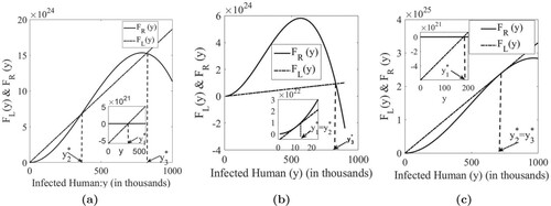$y_1^{\ast },y_2^{\ast },y_3^{\ast }$, are then given by the intersection of the curves $F_L\left(y\right)$ and $F_R\left(y\right)$ (Figure 3). As shown in Figure 3, the slope $-M_2$ of the linear function $F_L\left(y\right)$, which can be explained in terms of the infection rate ${\text{β}}_h$, can help determine the existence of 1, 2, or 3 equilibria. An increase in ${\text{β}}_h$ (i.e. a decrease in the slope of $F_L\left(y\right)$) makes the equilibrium point $y_1^{\ast }$ and $y_3^{\ast }$ move to the right and $y_2^{\ast }$ move to the left, eventually giving $y_1^{\ast }=y_2^{\ast }$ corresponding to two equilibria $y_1^{\ast }=y_2^{\ast }$ and $y_3^{\ast }$ (Figure 3(b)). Increasing ${\text{β}}_h$ further, $y_1^{\ast }$ and $y_2^{\ast }$ disappear, and only one equilibrium point $y_3^{\ast }$ exists. Since the equilibrium point $y_3^{\ast }$ attains the highest value, we can correspond this situation to the worst-case scenario, i.e. a high endemic level. Similarly, decreasing ${\text{β}}_h$ (i.e. increasing the slope of the linear function $F_L\left(y\right)$) causes $y_1^{\ast }$ and $y_3^{\ast }$ to move to the left and $y_2^{\ast }$ to move to the right. At some point, $y_2^{\ast }$ and $y_3^{\ast }$ coincide with each other, giving only two equilibrium points $y_1^{\ast }$ and $y_2^{\ast }=y_3^{\ast }$. If ${\text{β}}_h$ is decreased further, then $y_2^{\ast }$ and $y_3^{\ast }$ disappear, leaving only $y_1^{\ast }$ as an endemic equilibrium point. Since $y_1^{\ast }$ corresponds to the smallest equilibrium point, the case in which the only $y_1^{\ast }$ exists can be considered as the endemic condition with the minimum burden. Therefore, increasing the slope $-M_2$ (for example, decreasing ${\text{β}}_h$), making it less than its threshold value (corresponding to $y_2^{\ast }=y_3^{\ast }$), can be a vital control strategy to maintain the endemic at a low level.

Figure 3. Endemic equilibriums. (a) Graphs of $F_L\left(y\right)$ and $F_R\left(y\right)$ with possible three intersections corresponding to three endemic equilibrium points. (b) Graphs of $F_L\left(y\right)$ and $F_R\left(y\right)$ with exactly two endemic equilibrium points $y_1^{\ast }=y_2^{\ast }$ and $y_3^{\ast }$. Decreasing the slope of $F_L\left(y\right)$ further gives only one equilibrium point $y_3^{\ast }$ (a high epidemic level). (c) Graphs of $F_L\left(y\right)$ and $F_R\left(y\right)$ with exactly two endemic equilibrium points $y_1^{\ast }$ and $y_2^{\ast }=y_3^{\ast }$. Increasing the slope of $F_L\left(y\right)$ further gives only one equilibrium point $y_1^{\ast }$ (a low epidemic level).

In summary, the parameter $a_3$, which is always non-positive, provides an important threshold for disease-free equilibrium to occur ($a_3=0$). As long as $a_3\ne 0$ (i.e. $a_3<0$), there is no DFE, and the system always provides at least one endemic equilibrium. The absence of DFE with at least one endemic equilibrium can be attributable to ongoing infection abroad and the importation of malaria cases through cross-border mobility, making $a_3\ne 0$. When $a_3=0$ (presence of DFE), 1 or 2 endemic equilibrium points exist according to the sign of other parameters ($a_1$, $a_2$), which depend upon the thresholds $R_0,R_1,$ or $R_2$. Similarly, when $a_3<0$ (absence of DFE), 1 to 3 endemic equilibrium points exist according to the sign of other coefficients.

4.3. Stability analysis and uniform persistence

In this section, we provide some analytical results related to the stability and uniform persistence of the system, specifically, the local stability of the disease-free equilibrium points and the uniform persistence for Case-I and Case-II. In addition, for Case-III, we provide the local stability of the disease-free equilibrium point that corresponds to the absence of disease within the home country only. We were unable to prove the uniform persistence for Case-III and Case-IV because of the complexity of the model, presumably due to the absence of the overall disease-free equilibrium point in these cases.

4.3.1. Case-I: $\eta =0,\theta =0,k\ne 0$ (absence of cross-border mobility)

We prove the local stability of the disease-free equilibrium $E_0$ as stated in the following theorem.

Theorem 4.2

The disease free equilibrium point $E_0$ of the system (11(11) $\begin{array}{rl}{S}_{hH}^{\prime }& =\mathrm{\Lambda }+\eta S_{hM}+q{R}_{hH}-\frac{b{\alpha }_{vh}{I}_{vH}}{N_{hH}}{S}_{hH}-(\eta +d_h)S_{hH},\end{array}$(11) )–(18(18) $\begin{array}{rl}{R}_{hM}^{\prime }& ={\gamma }_h{I}_{hM}+\eta R_{hH}-(\eta +d_h+q)R_{hM}.\end{array}$(18) ) is locally asymptotically stable if $R_0<1$, and unstable if $R_0>1$.

Proof.

See Appendix A.6.

From the eigenvalues of the Jacobian matrix J at $E_0$ (Appendix A.6), we have the following lemma.

Lemma 4.3

For the Jacobian matrix J, the following statements hold:

1. $R_0=1$ if and only if $S\left(J\right)=0,$

2. $R_0>1$ if and only if $S\left(J\right)>0,$

3. $R_0<1$ if and only if $S\left(J\right)<0,$

where $S\left(J\right):=max\left\{\mathrm{R}\mathrm{e}\right(\lambda ):\lambda \text{is eigenvalue of the jacobian of system at DFE}{E}_0\}.$

We now establish that $R_0>1$ can also provide a condition for the uniform persistence of the disease in the home country in the absence of cross-border mobility. Here, we use the following notations and definitions. $\begin{array}{rl}& {\mathrm{\Omega }}_o=\{\left(S_{hH}\right(t),I_{hH}(t),\dots ,I_{vH}(t\left)\right)\in {\mathrm{\Re }}_{+}^5:S_{hH}(t)>0,I_{hH}(t)>0,\dots ,I_{vH}(t)>0\},\\ & \mathrm{\partial }{\mathrm{\Omega }}_o=\{\left(S_{hH}\right(t),I_{hH}(t),\dots ,I_{vH}(t\left)\right)\in {\mathrm{\Re }}_{+}^5:I_{hH}(t)=0\text{or}{I}_{vH}(t)=0\},\\ & \mathrm{\Omega }={\mathrm{\Omega }}_o\cup \mathrm{\partial }{\mathrm{\Omega }}_o={\mathrm{\Re }}_{+}^5.\end{array}$In the absence of cross-border mobility, it is enough to consider only the decoupled system (11(11) $\begin{array}{rl}{S}_{hH}^{\prime }& =\mathrm{\Lambda }+\eta S_{hM}+q{R}_{hH}-\frac{b{\alpha }_{vh}{I}_{vH}}{N_{hH}}{S}_{hH}-(\eta +d_h)S_{hH},\end{array}$(11) )–(15(15) $\begin{array}{rl}{I}_{vH}^{\prime }& =\frac{b{\alpha }_{hv}{I}_{hH}}{N_{hH}}{S}_{vH}-d_v{I}_{vH},\end{array}$(15) ). We assume that $\tau \left(t\right)P$ is the solution maps generated by the decoupled system (11(11) $\begin{array}{rl}{S}_{hH}^{\prime }& =\mathrm{\Lambda }+\eta S_{hM}+q{R}_{hH}-\frac{b{\alpha }_{vh}{I}_{vH}}{N_{hH}}{S}_{hH}-(\eta +d_h)S_{hH},\end{array}$(11) )–(15(15) $\begin{array}{rl}{I}_{vH}^{\prime }& =\frac{b{\alpha }_{hv}{I}_{hH}}{N_{hH}}{S}_{vH}-d_v{I}_{vH},\end{array}$(15) ) with initial value P. We denote $M_{\mathrm{\partial }}=\{P\in \mathrm{\partial }{\mathrm{\Omega }}_o:\tau (t)P\in \mathrm{\partial }{\mathrm{\Omega }}_o\}$, and $\omega \left(P\right)=\{y:\tau (t)P\to y\text{ as }t\to \mathrm{\infty }\}$. We first state and prove the following three lemmas.

Lemma 4.4

The sets ${\mathrm{\Omega }}_o$ and $\mathrm{\partial }{\mathrm{\Omega }}_o$ are positively invariant under the flow induced by the decoupled system (11(11) $\begin{array}{rl}{S}_{hH}^{\prime }& =\mathrm{\Lambda }+\eta S_{hM}+q{R}_{hH}-\frac{b{\alpha }_{vh}{I}_{vH}}{N_{hH}}{S}_{hH}-(\eta +d_h)S_{hH},\end{array}$(11) )–(15(15) $\begin{array}{rl}{I}_{vH}^{\prime }& =\frac{b{\alpha }_{hv}{I}_{hH}}{N_{hH}}{S}_{vH}-d_v{I}_{vH},\end{array}$(15) ) of the home country.

Proof.

See Appendix A.7.

Lemma 4.5

Every forward orbit of $\tau \left(t\right)$ in $M\mathrm{\partial }$ converge to $E_0$, i.e. $E_0$ is the fixed point of $\tau \left(t\right)$ and acyclic in $M\mathrm{\partial }$.

Proof.

See Appendix A.8.

Lemma 4.6

If $R_0>1$, then there exists $\rho >0$ such that $\underset{t\to \mathrm{\infty }}{lim}\text{Sup }\Vert \tau \left(t\right)P-E_0\Vert \ge \rho ,\mathrm{\forall }P\in {\mathrm{\Omega }}_o.$i.e. $E_0$ is uniform weak repeller with $\tau \left(t\right).$

Proof.

See Appendix A.9.

We are now ready to state the following theorem, which establishes the condition for malaria persistence in Nepal when cross-border mobility is absent.

Theorem 4.7

Let $R_0>1$, then the decoupled system (11(11) $\begin{array}{rl}{S}_{hH}^{\prime }& =\mathrm{\Lambda }+\eta S_{hM}+q{R}_{hH}-\frac{b{\alpha }_{vh}{I}_{vH}}{N_{hH}}{S}_{hH}-(\eta +d_h)S_{hH},\end{array}$(11) )–(15(15) $\begin{array}{rl}{I}_{vH}^{\prime }& =\frac{b{\alpha }_{hv}{I}_{hH}}{N_{hH}}{S}_{vH}-d_v{I}_{vH},\end{array}$(15) ) of home country is uniformly persistent with respect to $({\mathrm{\Omega }}_o,\mathrm{\partial }{\mathrm{\Omega }}_o)$ in the sense that there is a positive constant $\sigma >0$ such that every solution $\left(S_{hH}\right(t),I_{hH}(t),R_{hH}(t),S_{vH}(t),I_{vH}(t\left)\right)$ of (11(11) $\begin{array}{rl}{S}_{hH}^{\prime }& =\mathrm{\Lambda }+\eta S_{hM}+q{R}_{hH}-\frac{b{\alpha }_{vh}{I}_{vH}}{N_{hH}}{S}_{hH}-(\eta +d_h)S_{hH},\end{array}$(11) )–(15(15) $\begin{array}{rl}{I}_{vH}^{\prime }& =\frac{b{\alpha }_{hv}{I}_{hH}}{N_{hH}}{S}_{vH}-d_v{I}_{vH},\end{array}$(15) ) with $\left(S_{hH}\right(0),I_{hH}(0),R_{hH}(0),S_{vH}(0),I_{vH}(0\left)\right)\in {\mathrm{\Omega }}_o$ satisfies (25) $\underset{t\to \mathrm{\infty }}{lim}\text{Inf }{I}_{hH}\ge \sigma ,\underset{t\to \mathrm{\infty }}{lim}\text{Inf }{I}_{vH}\ge \sigma$(25)

Proof.

Assume that $R_0>1$, then it follows from Lemma 4.3 that $S\left(J\right)>0$. Let $\tau \left(t\right)P$ is the solution maps generated by the decoupled system (11(11) $\begin{array}{rl}{S}_{hH}^{\prime }& =\mathrm{\Lambda }+\eta S_{hM}+q{R}_{hH}-\frac{b{\alpha }_{vh}{I}_{vH}}{N_{hH}}{S}_{hH}-(\eta +d_h)S_{hH},\end{array}$(11) )–(15(15) $\begin{array}{rl}{I}_{vH}^{\prime }& =\frac{b{\alpha }_{hv}{I}_{hH}}{N_{hH}}{S}_{vH}-d_v{I}_{vH},\end{array}$(15) ) with initial value $P\in {\mathrm{\Omega }}_o$. Clearly, the system $\left\{\tau \right(t){\}}_{t\ge 0}$ admits the global attractor in ${\mathrm{\Re }}_{+}^5$. From the Lemma 4.5, $E_0$ is a fixed point of $\tau \left(t\right)$ and acyclic in $M\mathrm{\partial }$, every solution in $M\mathrm{\partial }$ approaches $E_0$. Moreover, Lemma 4.6 implies that $E_0$ is an isolated invariant set in Ω and $W^s\left(E_0\right)\cap {\mathrm{\Omega }}_o=\varphi$. By the acyclicity theorem of uniform persistence for maps [73], it follows that $\tau \left(t\right)$ is uniformly persistent with respect to $({\mathrm{\Omega }}_o,\mathrm{\partial }{\mathrm{\Omega }}_0)$. Hence there exists $\sigma >0$ such that $\underset{t\to \mathrm{\infty }}{lim}\text{Inf }{I}_{hH}\ge \sigma ,\underset{t\to \mathrm{\infty }}{lim}\text{Inf }{I}_{vH}\ge \sigma$. This completes the proof.

4.3.2. Case-II: $\eta \ne 0,\theta \ne 0,k=0$ (complete protection of transmission abroad)

The local stability of the disease-free equilibrium $E_{01}$, corresponding to the case when complete protection of transmission is in force outside Nepal, is given by the following theorem.

Theorem 4.8

The disease free equilibrium point $E_{01}$ of the system (11(11) $\begin{array}{rl}{S}_{hH}^{\prime }& =\mathrm{\Lambda }+\eta S_{hM}+q{R}_{hH}-\frac{b{\alpha }_{vh}{I}_{vH}}{N_{hH}}{S}_{hH}-(\eta +d_h)S_{hH},\end{array}$(11) )–(18(18) $\begin{array}{rl}{R}_{hM}^{\prime }& ={\gamma }_h{I}_{hM}+\eta R_{hH}-(\eta +d_h+q)R_{hM}.\end{array}$(18) ) is locally asymptotically stable if $R_1<1$, and unstable if $R_1>1$.

Proof.

See Appendix A.10.

We also have the following lemma.

Lemma 4.9

For the Jacobian matrix $J_1$ (Appendix A.10), the following statements hold:

1. $R_1=1$ if and only if $S\left(J_1\right)=0,$

2. $R_1>1$ if and only if $S\left(J_1\right)>0,$

3. $R_1<1$ if and only if $S\left(J_1\right)<0.$

We also prove that $R_1>1$ provides the condition for uniform persistence of the disease with dynamics given by the system (11(11) $\begin{array}{rl}{S}_{hH}^{\prime }& =\mathrm{\Lambda }+\eta S_{hM}+q{R}_{hH}-\frac{b{\alpha }_{vh}{I}_{vH}}{N_{hH}}{S}_{hH}-(\eta +d_h)S_{hH},\end{array}$(11) )–(18(18) $\begin{array}{rl}{R}_{hM}^{\prime }& ={\gamma }_h{I}_{hM}+\eta R_{hH}-(\eta +d_h+q)R_{hM}.\end{array}$(18) ) with $\eta \ne 0,\theta \ne 0,k=0$. Here, we use the following notations and definitions. $\begin{array}{rl}& {\mathrm{\Omega }}_o=\{\left(S_{hH}\right(t),I_{hH}(t),\dots ,R_{hM}(t\left)\right)\in {\mathrm{\Re }}_{+}^8:S_{hH}(t)>0,I_{hH}(t)>0,\dots ,R_{hM}(t)>0\},\\ & \mathrm{\partial }{\mathrm{\Omega }}_o=\{\left(S_{hH}\right(t),I_{hH}(t),\dots ,R_{hM}(t\left)\right)\in {\mathrm{\Re }}_{+}^8:I_{hH}(t)=0\text{or}{I}_{vH}(t)=0\text{or}{I}_{hM}(t)=0\}.\end{array}$To prove uniform persistence of $\left\{\tau \right(t){\}}_{t\ge 0}$ with respect to $({\mathrm{\Omega }}_o,\mathrm{\partial }{\mathrm{\Omega }}_o)$, we need the following three lemmas.

Lemma 4.10

The sets ${\mathrm{\Omega }}_o$ and $\mathrm{\partial }{\mathrm{\Omega }}_o$ are positively invariant under the flow induced by the system (11(11) $\begin{array}{rl}{S}_{hH}^{\prime }& =\mathrm{\Lambda }+\eta S_{hM}+q{R}_{hH}-\frac{b{\alpha }_{vh}{I}_{vH}}{N_{hH}}{S}_{hH}-(\eta +d_h)S_{hH},\end{array}$(11) )–(18(18) $\begin{array}{rl}{R}_{hM}^{\prime }& ={\gamma }_h{I}_{hM}+\eta R_{hH}-(\eta +d_h+q)R_{hM}.\end{array}$(18) ).

Proof.

See Appendix A.11.

Lemma 4.11

Every forward orbit of $\tau \left(t\right)$ in $M\mathrm{\partial }$ converge to $E_{01}.$

Proof.

See Appendix A.12

Lemma 4.12

If $R_1>1$, then there exists $\rho >0$ such that $\underset{t\to \mathrm{\infty }}{lim}\text{Sup }\Vert \tau \left(t\right)P-E_{01}\Vert \ge \rho ,\mathrm{\forall }P\in {\mathrm{\Omega }}_o.$i.e. $E_{01}$ is uniform weak repeller with $\tau \left(t\right).$

Proof.

See Appendix A.13.

With the help of the above lemmas, we now establish the following persistence theorem.

Theorem 4.13

If $R_1>1$, then the system (11(11) $\begin{array}{rl}{S}_{hH}^{\prime }& =\mathrm{\Lambda }+\eta S_{hM}+q{R}_{hH}-\frac{b{\alpha }_{vh}{I}_{vH}}{N_{hH}}{S}_{hH}-(\eta +d_h)S_{hH},\end{array}$(11) )–(18(18) $\begin{array}{rl}{R}_{hM}^{\prime }& ={\gamma }_h{I}_{hM}+\eta R_{hH}-(\eta +d_h+q)R_{hM}.\end{array}$(18) ) is uniformly persistent with respect to $({\mathrm{\Omega }}_o,\mathrm{\partial }{\mathrm{\Omega }}_o)$ in the sense that there is a positive constant $\sigma >0$ such that every solution $\left(S_{hH}\right(t),I_{hH}(t),R_{hH}(t),S_{vH}(t),I_{vH}(t),S_{hM}(t),I_{hM}(t),R_{hM}(t\left)\right)$ with $\left(S_{hH}\right(0),I_{hH}(0),R_{hH}(0),S_{vH}(0),I_{vH}(0),S_{hM}(0),I_{hM}(0),R_{hM}(0\left)\right)\in {\mathrm{\Omega }}_o$ satisfies $\underset{t\to \mathrm{\infty }}{lim}\text{Inf }{I}_{hH}\ge \sigma ,\underset{t\to \mathrm{\infty }}{lim}\text{Inf }{I}_{vH}\ge \sigma ,\underset{t\to \mathrm{\infty }}{lim}\text{Inf }{I}_{hA}\ge \sigma$.

Proof.

Assume that $R_1>1$, then it follows from Lemma 4.9 that $S\left(J_1\right)>0$. Let $\tau \left(t\right)P$ is the solution maps generated by the system (11(11) $\begin{array}{rl}{S}_{hH}^{\prime }& =\mathrm{\Lambda }+\eta S_{hM}+q{R}_{hH}-\frac{b{\alpha }_{vh}{I}_{vH}}{N_{hH}}{S}_{hH}-(\eta +d_h)S_{hH},\end{array}$(11) )–(18(18) $\begin{array}{rl}{R}_{hM}^{\prime }& ={\gamma }_h{I}_{hM}+\eta R_{hH}-(\eta +d_h+q)R_{hM}.\end{array}$(18) ) with the initial value P. Clearly, the system $\left\{\tau \right(t){\}}_{t\ge 0}$ admits the global attractor in ${\mathrm{\Re }}_{+}^8$. Here, the stable set of $E_{01}$ is $W^s\left(E_{01}\right)=\{P\in d(\tau \left(t\right)P,E_{01})\to 0\text{ as }t\to \mathrm{\infty }\}.$ From the Lemma 4.11, $E_{01}$ is a fixed point of $\tau \left(t\right)$ and acyclic in $M\mathrm{\partial }$, every solution in $M\mathrm{\partial }$ approach to $E_{01}$. Moreover, Lemma 4.12 implies that $E_{01}$ is an isolated invariant set in Ω and $W^s\left(E_{01}\right)\cap {\mathrm{\Omega }}_o=\varphi$. By the acyclicity theorem of uniform persistence for maps [73], it follows that $\tau \left(t\right)$ is uniformly persistent with respect to $({\mathrm{\Omega }}_o,\mathrm{\partial }{\mathrm{\Omega }}_0)$. Hence there exist $\sigma >0$ such that $\underset{t\to \mathrm{\infty }}{lim}\text{Inf }{I}_{hH}\ge \sigma ,\underset{t\to \mathrm{\infty }}{lim}\text{Inf }{I}_{hM}\ge \sigma ,\underset{t\to \mathrm{\infty }}{lim}\text{Inf }{I}_{vH}\ge \sigma .$ This completes the proof.

4.3.3. Case-III: $\eta \ne 0,\theta =0,k\ne 0$ (strict border screening and isolation)

In this case, the local stability of the corresponding disease-free equilibrium point, $E_{02}$, is given by the theorem below. As mentioned earlier, this disease-free equilibrium asserts the disease-free only within the home country while allowing infected migrants abroad.

Theorem 4.14

The disease free equilibrium point $E_{02}$ of the system (11(11) $\begin{array}{rl}{S}_{hH}^{\prime }& =\mathrm{\Lambda }+\eta S_{hM}+q{R}_{hH}-\frac{b{\alpha }_{vh}{I}_{vH}}{N_{hH}}{S}_{hH}-(\eta +d_h)S_{hH},\end{array}$(11) )–(18(18) $\begin{array}{rl}{R}_{hM}^{\prime }& ={\gamma }_h{I}_{hM}+\eta R_{hH}-(\eta +d_h+q)R_{hM}.\end{array}$(18) ) is locally asymptotically stable if $R_2<1$, and unstable if $R_2>1$.

Proof.

See Appendix A.14.

4.4. Analysis of simplifications implemented in the model

4.4.1. Approximation with autonomous sytem

Note that our model is non-autonomous due to the time-dependent parameter $\psi \left(t\right)$, representing the API of India. However, for analytical tractability (Subsections 4.1, 4.2, and 4.3), we approximated the model with the autonomous system. Moreover, since the future API of India can not be obtained, the simulation results for model prediction and control programmes (Section 5) are computed based on the autonomous model with the current API of India. In this section, we examine the potential error that we anticipate from the autonomous model. For this, we compared the predicted cumulative cases for both autonomous and non-autonomous systems for the period 2009–2019 (see in page-1 of Supplementary Material B). We observed that the predicted cumulative cases by the autonomous model remain within 5% of the non-autonomous model. For example, from 2009 to 2019, the difference in cumulative cases from the two model systems is only 1000 out of 20,000 base cases. Therefore, the autonomous model provides a reasonable approximation to the non-autonomous model, and the study's main finding remains the same in both models.

4.4.2. Approximations to the exposed class of mosquitoes and pathogen transmission from recovered humans

Because of the limited data availability, we have not included two potential phenomena: the incubation period of mosquitoes and pathogen transmission from recovered humans. However, these phenomena have been considered in some previous studies [15,47]. While these phenomena may not significantly impact the primary objective of this study, namely the impact of imported cases on the malaria elimination programme, we also considered an extended model with these two phenomena incorporated. Fitting this extended model to the data with the same initial values of state variables and parameters (Tables 1 and 2), we obtained the transmission probability from recovered human to susceptible mosquitoes per bite to be r = 0.35 and the incubation period of mosquito as $1/\sigma =10$ days, consistent with previous studies [15,34]. Notably, per capita mosquito biting rates of $b_1=56$ and $b_2=48$, estimated with the extended model, are within the 95% confidence interval of the estimates from the simplified model.

Table 1. Base value of demographic variables of malaria in Nepal.

Description	State variables	Base Value	Reference
Risk humans population in Nepal	$N_{hH}\left(0\right)$	9,756,426	Calculated
Susceptible humans in Nepal	$S_{hH}\left(0\right)$	9,754,000	Calculated
Infectious humans in Nepal	$I_{hH}\left(0\right)$	2000	Assumed
Recovered humans in Nepal	$R_{hH}\left(0\right)$	426	Assumed
Susceptible Migrants in India	$S_{hM}\left(0\right)$	1,898,300	[29]
Infectious Migrants in India	$I_{hM}\left(0\right)$	1400	Assumed
Recovered Migrants in India	$R_{hM}\left(0\right)$	300	Assumed
Susceptible mosquitoes in Nepal	$S_{vH}\left(0\right)$	9,754,176	Assumed
Infectious mosquitoes in Nepal	$I_{vH}\left(0\right)$	2250	Assumed

Table 2. Model parameters of incidence of malaria in Nepal.

Description	Parameters	Base value and unit	Reference
Probability of malaria transmission from an infectious mosquito (per bite) to a susceptible human	${\alpha }_{vh}$	0.0195	[1,13]
Probability of malaria transmission from an infectious human to a susceptible mosquito (per bite)	${\alpha }_{hv}$	0.63	[5,9,13]
Humans recruitment rate	Λ	287,460 Number $\times {\mathrm{y}\mathrm{r}}^{-1}$	Calculated
Per capita recovery rate of humans	${\gamma }_h$	1.85 ${\mathrm{y}\mathrm{r}}^{-1}$	[1,13]
Per capita natural birth and death rate of mosquitoes	$d_v$	27.9113 ${\mathrm{y}\mathrm{r}}^{-1}$	[1,13]
Per capita disease induced death rate of humans	${\delta }_h$	0.00171${\mathrm{y}\mathrm{r}}^{-1}$	Calculated
Per capita natural death rate of humans	$d_h$	0.0149${\mathrm{y}\mathrm{r}}^{-1}$	Calculated
Per capita mobility rate of healthy humans	η	0.0183${\mathrm{y}\mathrm{r}}^{-1}$	Calculated
Per capita disease import rate of humans	θ	0.98 ${\mathrm{y}\mathrm{r}}^{-1}$	Estimated
		[0.4172, 1.5428]
Per capita disease export rate of humans	p	$0{\mathrm{y}\mathrm{r}}^{-1}$	Assumed
Per capita rate of Immunity loss of humans	q	4 ${\mathrm{y}\mathrm{r}}^{-1}$	[15]
Parameter related with incidence rate in India	ζ	$0.00105{\mathrm{y}\mathrm{r}}^{-1}$	Estimated
		[0.0005, 0.0016]
Per capita biting rate of mosquitoes at home country up to 2014	$b_1$	48 ${\mathrm{y}\mathrm{r}}^{-1}$	Estimated
		[39.6537, 66.3463]
Per capita biting rate of mosquitoes at home country after 2014	$b_2$	39.5 ${\mathrm{y}\mathrm{r}}^{-1}$	Estimated
		[29.6318, 49.3682]

Moreover, the cumulative case during 2020–2026 predicted by the extended model is 1425, which is close to the estimate of 1348 by the simplified model. Similarly, the predicted new cases in the year 2026 by the extended model is 195, while that by the simplified model is 191. Therefore, the qualitative and quantitative differences between the two models with and without the exposed class of mosquitoes and pathogen transmission from recovered humans are not significant, asserting the robustness of the simplified models(see in page 2-4 of Supplementary Material B).

5. Malaria epidemic prediction and potential control in Nepal: model simulations

We use our model to predict the malaria epidemic in Nepal and evaluate the potential control strategies. In particular, we focus on whether the goal of malaria elimination from Nepal by 2026 set by the Government of Nepal can be achieved with the current trend and/or potential strategies. We take the year 2020 as the base year and estimate the imported and indigenous malaria cases during the period 2020–2026, and assess the number of possible control strategies that can be implemented for malaria elimination.

5.1. Basic malaria epidemic outcome in Nepal

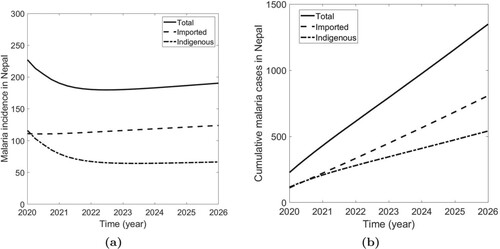
For the basic simulations, we take the API of India, $\psi \left(t\right)$, a constant value corresponding to the year 2018. We compute the model predicted values of indigenous and imported new cases for 2020–2026 (Figure 4(a)). We observe that if the current trend continues, the indigenous malaria cases follow a decreasing trend, but the imported cases increase slightly. We predict the indigenous malaria cases in Nepal will decrease to a yearly incidence of 67 cases in 2026, while the imported cases will remain 124 per year in 2026. As a result, the annual total incidence will remain 191 cases in the year 2026. With this incidence rate, the cumulative indigenous cases and imported cases for the period 2020 to 2026 will reach 540 and 808, respectively, making a total of 1348 cases of malaria in Nepal in this period (Figure 4(b)). While the magnitude remains relatively low, a slightly elevated level of new cases in 2026, mainly because of the imported cases, shows that the importation of malaria cases from India might remain an obstacle to the Nepal government's goal of malaria elimination by 2026.

Figure 4. Model prediction of the malaria epidemic in Nepal. (a) The model prediction of the annual incidence of indigenous, imported, and total malaria cases from 2020 to 2026; and (b) the model prediction of the cumulative cases of indigenous, imported and total malaria infection from 2020 to 2026.

5.2. Impact of the transmission abroad on the epidemic in home country

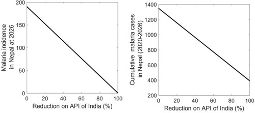
As revealed in the model-predicted epidemic trend, the transmission of malaria abroad that may eventually cause higher imported cases can be a determinant factor for achieving an elimination goal by 2026. The model parameter k, which represents the impact of API of India, can be used to study how the transmission dynamics abroad can impact the epidemic outcome in Nepal. According to the data API of India has had a decreasing trend for the last few years. If the decreasing trend continues, imported cases in Nepal are expected to reduce in the coming years. Our model predicts that the malaria incidence in the year 2026 decreases linearly as the % reduction of API of India increases (Figure 5). For example, reducing the current API (base value k = 0.1) by 50% brings down the annual malaria incidence from 191 to 95 in 2026. The linear dependency of cumulative cases on the % reduction of India's API is also seen with a 50% reduction from the base case bringing the cumulative cases from 1,348 to 869 during the period 2020–2026 (Figure 5). These results indicate that the API of India can have an important role in the cases in the home country and eventually on the success of the Nepal government's malaria elimination goal.

Figure 5. Impact of the API of India. Reduction of total malaria incidence at the year 2026 (Left) and reduction of cumulative malaria cases from 2020–2026 (Right) with Annual Parasitic Incidence (API) of India taking its value 0.1 for the base year 2020.

5.3. Control of malaria in Nepal

We consider four potential control strategies: (1) Insecticide-treated nets (ITN), (2) Indoor Residual Spraying (IRS), (3) Border screen and isolation (BSI), and (4) Migration reduction (MR). Implementation of ITN reduces the mosquito biting rate. Assuming ${\varphi }_{ITN}$ represents the effectiveness of ITN (assuming 100% coverage), the implementation of this strategy transforms $b\to (1-{\varphi }_{ITN})b$ in our model. Similarly, IRS increases mosquito death, transforming our model as $d_v\to {\varphi }_{IRS}{d}_v$, where ${\varphi }_{IRS}\ge 1$ is the enhancement of mosquito death rate due to IRS. We denote the effectiveness of BSI by ${\varphi }_{BSI}$, $0\le {\varphi }_{BSI}\le 1$ so that the implementation of this strategy results in the transformation $\theta \to (1-{\varphi }_{BSI})\theta$, i.e. reduction of the disease import rate θ by a proportion ${\varphi }_{BSI}$. The last strategy, MR, can be attributed to promoting various employment opportunities within the country, thereby reducing the cross-border mobility for seeking employment in India. The strategies can be incorporated into our model by transforming $\eta \to (1-{\varphi }_{MR})\eta ,\theta \to (1-{\varphi }_{MR})\theta$, where ${\varphi }_{MR}$, $0\le {\varphi }_{MR}\le 1$ is the effectiveness of MR.

The mosquito biting rate is one of the most critical parameters of malaria transmission. While we estimated the low biting rate from the data fitting, the estimated value is the average annual rate. In reality, the biting rate can be uncertain as it is affected by various environmental (seasonal), social, and economic factors. To include broader possible scenarios, we present the results for two different biting rates, low biting rate (base case b = 39.5 and high biting rate (approximately two times higher than the base case, b = 100).

5.3.1. Control strategies for elimination

The analytical results that we proved in Subsection 4.2 inform us that malaria can be eliminated from the home country if one of the following conditions can be achieved: absence of cross-border mobility (case I in Subsection 4.2.1), full protection of transmission abroad (case II in Subsection 4.2.2), and strict border screening and isolation (case III in Subsection 4.2.3). According to our theorems, in case I, II, and III, the malaria gets eliminated if ($R_0<1,a_{10}>0$), ($R_1<1,a_{11}>0$), and ($R_2<1,a_{12}>0$), respectively, where $a_{10},a_{11}$, and $a_{12}$ are corresponding values of $a_1$ for case I, II, and III, respectively. We now evaluate whether the control strategies (${\varphi }_{ITN},{\varphi }_{IRS},{\varphi }_{BSI},$ and ${\varphi }_{MR}$) can bring the model to satisfy the condition of eliminating malaria in Nepal.

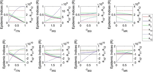
Our results show that for the low biting rate condition, the elimination of malaria can be achieved in Nepal regardless of whether any of the control strategies are applied or not because $R_0<1,R_1<1,R_2<1$ and $a_{10}>0,a_{11}>0,a_{12}>0$ remain always true (Figure 6, first row). However, for the high biting rate condition, $R_0<1,R_1<1,R_2<1$ and $a_{10}>0,a_{11}>0,a_{12}>0$ can not be achieved without the control strategies, i.e. for ${\varphi }_{ITN}={\varphi }_{BSI}={\varphi }_{MR}=0$, and ${\varphi }_{IRS}=1$ (Figure 6, second row). In this case, $\left({\varphi }_{BSI}\right)$ and $\left({\varphi }_{MR}\right)$ have no impact on R and $a_1$. Therefore, the control strategies related to the infected migrant workers and the mobility across the border are not enough for malaria elimination if the biting rate is high. In the high biting rate condition, ($R_0<1,a_{10}>0$), ($R_1<1,a_{11}>0$), and ($R_2<1,a_{12}>0$), i.e. the elimination of malaria, can be obtained if the level of ${\varphi }_{ITN}$ is greater than 0.35, 0.65, and 0.35, respectively, or the level of ${\varphi }_{IRS}$ is greater than 1.45, 2.60, 1.50, respectively (Figure 6, second row).

Figure 6. Condition for malaria elimination in Nepal. Threshold indices $R_0$, $R_1$, $R_2$, $a_{10}$, $a_{11}$, $a_{12}$ as a function of controls ${\varphi }_{ITN},{\varphi }_{IRS},{\varphi }_{BSI}$, and ${\varphi }_{MR}$ for a low (first row) and high (second row) mosquito biting conditions. Note that the malaria is eliminated if $R_0<1,a_{10}>0$, $R_1<1,a_{11}>0$, and $R_2<1,a_{12}>0$, respectively, where $a_{10},a_{11}$, and $a_{12}$ are corresponding values of $a_1$ for case I (absence of cross-border mobility), case II (full protection of transmission abroad), and case III (strict border screening and isolation), respectively.

5.3.2. Control strategies for minimal burden

Here we perform simulations to show how the control strategies ITN, IRS, BSI, and MR impact the annual malaria incidence in 2026 and the cumulative malaria cases for 2020–2026 (Figures 7 and 8). In the low mosquito biting rate condition (Figure 7, first row), our model predicts that the 50% effectiveness of ITN (i.e. ${\varphi }_{ITN}=0.5$) reduces the annual malaria incidence in the year 2026 from 191 to 135. As a result, the cumulative cases for 2020–2026 will be reduced from 1348 to 1001 (Figure 8, first row). An increase in IRS by 1.5 times (i.e. ${\varphi }_{IRS}=1.5$) will result in an annual incidence rate of 161 in 2026 and a cumulative cases of 1167 for 2020–2026. Similarly, 50% effectiveness of BSI and MR will reduce the annual incidence rate in the year 2026 to 114 and 100, respectively, and the cumulative cases for 2020–2026 to 903 and 889, respectively.

Figure 7. Effects of control strategies on the annual incidence rate. The model-predicted annual incidence rate in the year 2026 for various levels of ITN, IRS, BSI, and MR control in a low biting rate scenario (first row) and a high biting rate scenario (second row).

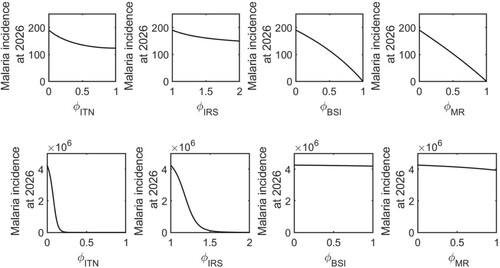
Figure 8. Effects of control strategies on the cumulative cases. The model-predicted cumulative cases for 2020–2026 for various levels of ITN, IRS, BSI, and MR control in a low biting rate scenario (first row) and a high biting rate scenario (second row).

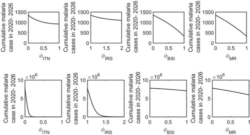
In a high mosquito biting rate condition (Figure 7, second row, and Figure 8, second row), our model predicts that the 50% effectiveness of ITN (i.e. ${\varphi }_{ITN}=0.5$) reduces the annual malaria incidence in the year 2026 from 4.25 million to 257 and the cumulative cases for 2020–2026 from 7.8 million to 1684. Similarly, an increase in IRS by 1.5 times (i.e. ${\varphi }_{IRS}=1.5$) will result in an annual incidence rate of 106 hundred thousand in 2026 and a cumulative cases of 128 hundred thousand for 2020–2026. 50% effectiveness of BSI and MR will reduce the annual incidence rate in the year 2026 to 4.23 million and 4.13 million, respectively, and the cumulative cases for 2020–2026 to 7.5 million and 6.98 million, respectively.

While each control strategy can maintain a minimum malaria burden, their effect may vary quantitatively. Among these control strategies, MR appears to be the most effective in controlling malaria in Nepal in low mosquito biting rate conditions, while ITN is the most effective control in the high biting rate condition. This indicates that the ideal control strategy may depend on the locations and seasons in which low or high mosquito biting rates are expected. We note that due to the existing open border relationship with a long history between Nepal and India, reducing the cross-border mobility of migrant workers may not be a viable option to implement. Therefore, the optimal border screen and isolation of returning migrant workers along with local approaches, ITN and IRS, can be the most impactful option for controlling and possibly eliminating malaria in Nepal.

In the above calculation, we assumed the 100% coverage of ITN. However, 100% is unlikely to be achieved, especially in resource-limited countries like Nepal. Thus we further observe model prediction for varying coverage and efficacy of ITN. 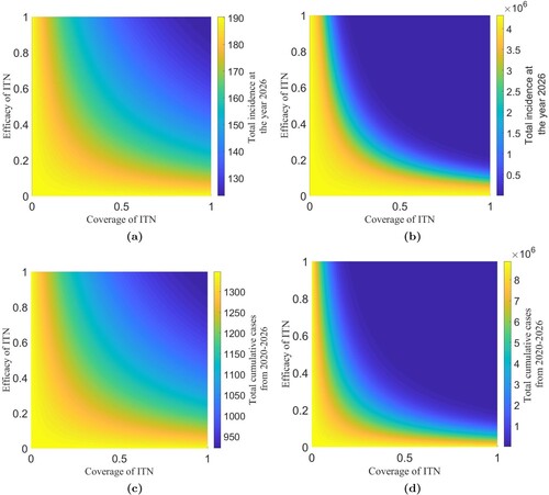The proportion of coverage ${\psi }_{ITN}$, $0\le {\psi }_{ITN}\le 1$, and efficacy ${\varphi }_{ITN}$, $0\le {\varphi }_{ITN}\le 1$, can be incorporated in our model transforming $b\to (1-{\varphi }_{ITN}{\psi }_{ITN})b.$ As presented in Figure 9, our simulations show that 100% efficacy and 100% coverage of ITN significantly reduce the malaria cases in the high mosquito biting case, but the effect is not significant in the low mosquito biting case. Since Nepal's estimated mosquito biting rate is low, even the 100% coverage and 100% efficacy will reduce malaria cases in 2026 from 191 to 121 only. Thus, in addition to ITN, optimal control strategies should also focus on adequately managing imported cases to eliminate malaria from Nepal by 2026.

Figure 9. Sensitivity of coverage and efficacy of ITN. The model-predicted annual incidence rate in 2026 for various levels of efficacy and coverage of ITN in a low biting rate scenario (a) and a high biting rate scenario (b). The model-predicted cumulative cases for 2020–2026 for various levels of efficacy and coverage of ITN in a low biting rate scenario (c) and a high biting rate scenario (d).

6. Conclusion

Despite a significant decline of malaria cases worldwide, many countries are currently facing difficulty achieving malaria elimination goals from those countries, mainly due to cross-border mobility of migrant workers potentially bringing malaria from abroad. Nepal provides a typical example, which is recently suffering from higher imported cases from India through open-border, posing a severe threat to the Nepal government's goal of eliminating malaria by 2026. In this study, we developed a novel mathematical model validated by the data from Nepal and used our model to analyze the effects of cross-border mobility on the malaria elimination programmes for low-endemic countries like Nepal.

Our model analyzes and simulations show that malaria can be eliminated from Nepal if strategies promoting the absence of cross-border mobility, complete protection of transmission abroad, or strict border screening and isolation are implemented. In each of these potential strategies, we formulated threshold conditions for the stability of the disease-free equilibriums, providing the level of control strategies, such as ITN, IRS, BSI, and MR, to assert the elimination of malaria from Nepal. In some cases, we mathematically proved the persistence of malaria in Nepal. In one of the cases, namely strict border screening and isolation, our unique model can provide the disease-free condition only within the home country while allowing the disease among migrants abroad. In reality, such disease-free equilibrium is the most viable condition regarding the elimination of malaria from Nepal because achieving elimination from both countries can be challenging with the control strategies by the Nepal government's policy only without making combined strategies by both countries. In addition, we used our model to thoroughly assess all control strategies considered, ITN, IRS, BSI, and MR, to maintain the low level of malaria-endemic in both low and high mosquito biting rate scenarios. Interestingly, our model predicts that MR is the most effective control strategy for the low mosquito biting rate condition, while ITN is the most effective control strategy for the high mosquito biting rate condition. These interesting results suggest that the best control strategy may depend on locations and seasons that determine whether the biting rate is low or high.

There are several limitations of our study. We approximated the incidence rate abroad (India) using the API data of India. The analysis of the full model with accurate dynamics of humans and mosquitoes abroad, along with data from India, can help improve our results. Although the frequent movement of humans and mosquitoes between bordering cities and the movement of mosquitoes through cross-border transportation may be important, we have not considered these factors in our model because the data of imported cases due to these movements are not available. Therefore, our results are more relevant to the infection importation through cross-border mobility of migrant workers. Our model parameters are estimated with the limited data of malaria cases in Nepal. Uncertainty on the model parameters can be clarified if more frequent data are available. While we estimated the mosquito population based on the previous studies, the implemented values may have some uncertainties. However, our further simulations show that changing the mosquito population size to a realistic limit does not significantly impact on the main qualitative conclusions of our study. Also, some districts of Nepal are directly connected with India making them more vulnerable in comparison to other areas. Therefore, an extension of our model may be necessary to incorporate the spatial heterogeneity of the malaria risk across districts of Nepal.

We also note that we could not prove the persistence theory in Case III (strict border screening and isolation) and Case IV (presence of cross-border mobility, no protection, and no border screening or isolation) because there is no complete disease-free equilibrium in these cases. Extensive mathematical theory may be needed to show the persistence of the disease in such complicated cases. Our analyses show that for some choice of parameters (for example, those making $a_1<0$), the disease may persist even if the threshold numbers $R_0$ (Case I in Subsection 4.2.1), $R_1$ (Case II in Subsection 4.2.2), and $R_2$ (Case III in Subsection 4.2.3) are less than 1, indicating a possibility of backward bifurcations. Therefore, a detailed bifurcation analysis for each case (I, II, and III) can be an essential work, which we plan to pursue in future research.

In summary, our model for malaria transmission dynamics, incorporating cross-border mobility between a low endemic country (Nepal) and a high endemic country (India), can provide important insights into an obstacle that cross-border mobility may create to malaria elimination programmes. Our analytical and simulation results informing control policies that bring malaria elimination or maintain the epidemic at a low level are helpful for policymakers if implemented in conjunction with more accurate data.

Acknowledgements

This research was supported by the GRAID (Graduate Research Assistantships in Developing Countries) awards from the International Mathematical Union (IMU). RG acknowledges the University Grants Commission (UGC) for Ph.D. Faculty Fellowship and the Nepal Mathematical Society (NMS) for the NMS Ph.D. Fellowship Award 2020. KA acknowledges the Nepal Academy of Science and Technology (NAST) for Ph.D. Fellowship and the Nepal Mathematical Society (NMS) for the NMS Ph.D. Fellowship Award 2020. AP acknowledges the Nepal Mathematical Society (NMS) for the NMS Ph.D. Fellowship Award 2020. The work of NV was supported by NSF grants DMS-1951793, DMS-1616299, DMS-1836647, and DEB-2030479 from the National Science Foundation of USA, and the UGP Award from San Diego State University.

Disclosure statement

No potential conflict of interest was reported by the author(s).

Additional information

Funding

This research was supported by the GRAID (Graduate Research Assistantships in Developing Countries) awards from the International Mathematical Union (IMU). RG acknowledges the University Grants Commission (UGC) for Ph.D.Faculty Fellowship and the Nepal Mathematical Society (NMS) for the NMS Ph.D. Fellowship Award 2020. KA acknowledges the Nepal Academy of Science and Technology (NAST) for Ph.D. Fellowship and the Nepal Mathematical Society (NMS) for the NMS Ph.D. Fellowship Award 2020. AP acknowledges the Nepal Mathematical Society (NMS) for the NMS Ph.D. Fellowship Award 2020. The work of NV was supported by NSF grants DMS-1951793, DMS-1616299, DMS-1836647, and DEB-2030479 from the National Science Foundation of USA, and the UGP Award from San Diego State University.

Appendices

Appendix 1

A.1. Proof of Theorem 4.1

First, we prove that all the solutions are bounded. From Equations (11(11) $\begin{array}{rl}{S}_{hH}^{\prime }& =\mathrm{\Lambda }+\eta S_{hM}+q{R}_{hH}-\frac{b{\alpha }_{vh}{I}_{vH}}{N_{hH}}{S}_{hH}-(\eta +d_h)S_{hH},\end{array}$(11) ), (12(12) $\begin{array}{rl}{I}_{hH}^{\prime }& =\frac{b{\alpha }_{vh}{I}_{vH}}{N_{hH}}{S}_{hH}+\theta I_{hM}-(p+d_h+{\delta }_h+{\gamma }_h)I_{hH},\end{array}$(12) ), and (13(13) $\begin{array}{rl}{R}_{hH}^{\prime }& ={\gamma }_h{I}_{hH}+\eta R_{hM}-(\eta +d_h+q)R_{hH},\end{array}$(13) ), we get $\begin{array}{rl}\frac{\mathrm{d}{S}_{hH}}{\mathrm{d}t}& =\mathrm{\Lambda }+q{R}_{hH}+\eta S_{hM}-\frac{b{\alpha }_{vh}{S}_{hH}{I}_{vH}}{N_{hH}}-(\eta +d_h)S_{hH}\\ & >-\frac{b{\alpha }_{vh}{S}_{hH}{I}_{vH}}{N_{hH}}-(\eta +d_h)S_{hH}\\ \Rightarrow S_{hH}& >S_{hH}\left(0\right)\exp \left(-{\int }_0^t(\frac{b{\alpha }_{vh}{I}_{vH}}{N_{hH}}+\eta +d_h)\mathrm{d}t\right)\ge 0;\\ \frac{\mathrm{d}{I}_{hH}}{\mathrm{d}t}& =\frac{b{\alpha }_{vh}{S}_{hH}{I}_{vH}}{N_{hH}}+\theta I_{hM}-(\theta +d_h+{\delta }_h+{\gamma }_h)I_{hH}\ge -(\theta +d_h+{\delta }_h+{\gamma }_h)I_{hH}\\ \Rightarrow I_{hH}& \ge I_{hH}\left(0\right)\exp \left(-{\int }_0^t(\theta +d_h+{\delta }_h+{\gamma }_h)\mathrm{d}t\right)\ge 0;\\ \text{and}\frac{\mathrm{d}{R}_{hH}}{\mathrm{d}t}& ={\gamma }_h{I}_{hH}+\eta R_{hA}-(\eta +d_h+q)R_{hH}\ge -(\eta +d_h+q)R_{hH}\\ \Rightarrow R_{hH}& \ge R_{hH}\left(0\right)\exp \left(-{\int }_0^t(\eta +d_h+q)\mathrm{d}t\right)\ge 0.\end{array}$Similarly, from Equations (16(16) $\begin{array}{rl}{S}_{hM}^{\prime }& =\eta S_{hH}+q{R}_{hM}-\zeta \psi \left(t\right)S_{hM}-(d_h+\eta )S_{hM},\end{array}$(16) ), (17(17) $\begin{array}{rl}{I}_{hM}^{\prime }& =\zeta \psi \left(t\right)S_{hM}+p{I}_{hH}-(\theta +{\delta }_h+d_h+{\gamma }_h)I_{hM},\end{array}$(17) ), and (18(18) $\begin{array}{rl}{R}_{hM}^{\prime }& ={\gamma }_h{I}_{hM}+\eta R_{hH}-(\eta +d_h+q)R_{hM}.\end{array}$(18) ), we get $\begin{array}{rl}\frac{\mathrm{d}{S}_{hM}}{\mathrm{d}t}& =\eta S_{hH}+q{R}_{hM}-(k+d_h+\eta )S_{hM}\ge -(k+d_h+\eta )S_{hM}\\ \Rightarrow S_{hM}& \ge S_{hM}\left(0\right)\exp \left(-{\int }_0^t(\eta +k+d_h)\mathrm{d}t\right)\ge 0;\\ \frac{\mathrm{d}{I}_{hM}}{\mathrm{d}t}& =k{S}_{hM}+\theta I_{hH}-(\theta +{\delta }_h+d_h+{\gamma }_h)I_{hM}\ge -(\theta +{\delta }_h+d_h+{\gamma }_h)I_{hM}\\ \Rightarrow I_{hM}& \ge I_{hM}\left(0\right)\exp \left(-{\int }_0^t(\theta +d_h+{\delta }_h+{\gamma }_h)\mathrm{d}t\right)\ge 0;\\ \text{and}\frac{\mathrm{d}{R}_{hM}}{\mathrm{d}t}& ={\gamma }_h{I}_{hM}+\eta R_{hH}-(\eta +d_h)R_{hM}\ge -(\eta +d_h+q)R_{hM}\\ \Rightarrow R_{hM}& \ge R_{hM}\left(0\right)\exp \left(-{\int }_0^t(\eta +d_h+q)\mathrm{d}t\right)\ge 0.\end{array}$Also, from (14(14) $\begin{array}{rl}{S}_{vH}^{\prime }& =\varphi -\frac{b{\alpha }_{hv}{I}_{hH}}{N_{hH}}{S}_{vH}-d_v{S}_{vH},\end{array}$(14) ) and (15(15) $\begin{array}{rl}{I}_{vH}^{\prime }& =\frac{b{\alpha }_{hv}{I}_{hH}}{N_{hH}}{S}_{vH}-d_v{I}_{vH},\end{array}$(15) ), $\begin{array}{rl}\frac{\mathrm{d}{S}_{vH}}{\mathrm{d}t}& =\varphi -\frac{b{\alpha }_{hv}{S}_{vH}{I}_{hH}}{N_{hH}}-d_v{S}_{vH}>-\frac{b{\alpha }_{hv}{S}_{vH}{I}_{hH}}{N_{hH}}-d_v{S}_{vH}\\ \Rightarrow S_{vH}& >S_{vH}\left(0\right)\exp \left(-{\int }_0^t(\frac{b{\alpha }_{hv}{I}_{hH}}{N_{hH}}+dv)\mathrm{d}t\right)\ge 0;\\ \text{and}\frac{\mathrm{d}{I}_{vH}}{\mathrm{d}t}& =\frac{b{\alpha }_{hv}{S}_{vH}{I}_{hH}}{N_{hH}}-d_v{I}_{vH}\ge -d_v{I}_{vH}\\ \Rightarrow I_{vH}& \ge I_{vH}\left(0\right)\exp \left(-{\int }_0^t\left(d_v\right)\mathrm{d}t\right)\ge 0.\end{array}$Hence the solution set $\left\{\right(S_{hH}\left(t\right),I_{hH}\left(t\right),R_{hH}\left(t\right),S_{hM}\left(t\right),I_{hM}\left(t\right),R_{hM}\left(t\right),S_{vH}\left(t\right),I_{vH}\left(t\right)\left)\right\}$ of the system (11(11) $\begin{array}{rl}{S}_{hH}^{\prime }& =\mathrm{\Lambda }+\eta S_{hM}+q{R}_{hH}-\frac{b{\alpha }_{vh}{I}_{vH}}{N_{hH}}{S}_{hH}-(\eta +d_h)S_{hH},\end{array}$(11) )–(18(18) $\begin{array}{rl}{R}_{hM}^{\prime }& ={\gamma }_h{I}_{hM}+\eta R_{hH}-(\eta +d_h+q)R_{hM}.\end{array}$(18) ) is always non-negative. We now prove that these non-negative solutions are bounded. Adding (11(11) $\begin{array}{rl}{S}_{hH}^{\prime }& =\mathrm{\Lambda }+\eta S_{hM}+q{R}_{hH}-\frac{b{\alpha }_{vh}{I}_{vH}}{N_{hH}}{S}_{hH}-(\eta +d_h)S_{hH},\end{array}$(11) )–(13(13) $\begin{array}{rl}{R}_{hH}^{\prime }& ={\gamma }_h{I}_{hH}+\eta R_{hM}-(\eta +d_h+q)R_{hH},\end{array}$(13) ) and (16(16) $\begin{array}{rl}{S}_{hM}^{\prime }& =\eta S_{hH}+q{R}_{hM}-\zeta \psi \left(t\right)S_{hM}-(d_h+\eta )S_{hM},\end{array}$(16) )–(18(18) $\begin{array}{rl}{R}_{hM}^{\prime }& ={\gamma }_h{I}_{hM}+\eta R_{hH}-(\eta +d_h+q)R_{hM}.\end{array}$(18) ), we obtain $\frac{\mathrm{d}{N}_h}{\mathrm{d}t}=\mathrm{\Lambda }-d_h{N}_h-{\delta }_h{I}_{hH}-{\delta }_h{I}_{hM}\le \mathrm{\Lambda }-d_h{N}_h,$which implies $\underset{t\to \mathrm{\infty }}{lim}{N}_h\le \frac{\mathrm{\Lambda }}{d_h}$. Hence, the human population, $N_h\left(t\right)$, is ultimately bounded.

Again, adding (14(14) $\begin{array}{rl}{S}_{vH}^{\prime }& =\varphi -\frac{b{\alpha }_{hv}{I}_{hH}}{N_{hH}}{S}_{vH}-d_v{S}_{vH},\end{array}$(14) ) and (15(15) $\begin{array}{rl}{I}_{vH}^{\prime }& =\frac{b{\alpha }_{hv}{I}_{hH}}{N_{hH}}{S}_{vH}-d_v{I}_{vH},\end{array}$(15) ), we obtain $\frac{\mathrm{d}{N}_v}{\mathrm{d}t}=\varphi -d_v{N}_v,$which implies $\underset{t\to \mathrm{\infty }}{lim}{N}_v=\frac{\varphi }{d_v}$. Hence, the mosquito population $N_v\left(t\right)$ is ultimately bounded. Thus all state variables representing the populations are non-negative and bounded.

A.2. Derivation of the epidemic index $R_0$ from the next generation matrix method

From the system (11(11) $\begin{array}{rl}{S}_{hH}^{\prime }& =\mathrm{\Lambda }+\eta S_{hM}+q{R}_{hH}-\frac{b{\alpha }_{vh}{I}_{vH}}{N_{hH}}{S}_{hH}-(\eta +d_h)S_{hH},\end{array}$(11) )–(18(18) $\begin{array}{rl}{R}_{hM}^{\prime }& ={\gamma }_h{I}_{hM}+\eta R_{hH}-(\eta +d_h+q)R_{hM}.\end{array}$(18) ), the newly infectious matrix $F_i$ and its Jacobian matrix F at the disease-free equilibrium point $E_0$ are $F_i=\left(\begin{array}{c}{\displaystyle \frac{{\text{β}}_h{S}_{hH}{I}_{vH}}{N_{hH}}}\\ {\displaystyle \frac{{\text{β}}_v{S}_{vH}{I}_{hH}}{N_{hH}}}\\ k{S}_{hM}\end{array}\right),F=\left(\begin{array}{ccc}0& {\text{β}}_h& 0\\ {\displaystyle \frac{{\text{β}}_v\varphi d_h}{\mathrm{\Lambda }{d}_v}}& 0& 0\\ 0& 0& 0\end{array}\right).$Again, the transfer matrix $V_i$ and its Jacobian matrix V at the disease-free equilibrium point, $V_i=\left(\begin{array}{c}(\theta +{\delta }_h+{\gamma }_h+d_h)I_{hH}-\theta I_{hM}\\ d_v{i}_{vH}\\ (\theta +{\gamma }_h+{\delta }_h+d_h)I_{hA}-\theta I_{hH}\end{array}\right),V=\left(\begin{array}{ccc}{d}_h+{\delta }_h+{\gamma }_h& 0& 0\\ 0& d_v& 0\\ 0& 0& {\gamma }_h+{\delta }_h+d_h\end{array}\right).$Here the dominant eigenvalue of $F{V}^{-1}$ gives the following epidemic index. $R_0=\sqrt{\frac{\varphi d_h{\text{β}}_h{\text{β}}_v}{(d_h+{\gamma }_h+{\delta }_h)\mathrm{\Lambda }{d}_v^2}}.$

A.3. Derivation of $R_0$ from the first principle method

The overall basic reproduction number ($R_0$) of malaria is equal to the geometric mean of the basic reproduction numbers of malaria transmission from an infected human to susceptible mosquitoes $\left(R_H\right)$ and the transmission of malaria from an infected mosquito to susceptible humans $\left(R_V\right)$. Here $\frac{b}{N_{hH}}$ is the average number of bites made by a mosquito to a human in unit time. Each mosquito bites at a constant rate, whereas the rate at which humans are bitten will vary with respect to the density of mosquitoes within the area. The expected number of infected mosquitoes from an infected human in his infectious period (assuming that all mosquitoes are susceptible) is given by $R_H=\frac{b{\alpha }_{hv}{N}_v^0}{(d_h+{\delta }_h+{\gamma }_h)N_h^0}=\frac{b{\alpha }_{hv}\varphi d_h}{(d_h+{\delta }_h+{\gamma }_h)\mathrm{\Lambda }{d}_v}$. Similarly, the expected number of susceptible humans that become infected due to contact with one infected mosquito in its infectious period (assuming that all humans are susceptible) are given by $R_V=\frac{b{\alpha }_{vh}{N}_h^0}{N_h^0{d}_v}=\frac{b{\alpha }_{vh}}{d_v}$. Then, we get $R_0=\sqrt{R_H\times R_V}=\sqrt{\frac{\varphi d_h{\text{β}}_h{\text{β}}_v}{\mathrm{\Lambda }(d_h+{\delta }_h+{\gamma }_h)d_v^2}}.$

A.4. Derivation of the epidemic index $R_1$

From the system (11(11) $\begin{array}{rl}{S}_{hH}^{\prime }& =\mathrm{\Lambda }+\eta S_{hM}+q{R}_{hH}-\frac{b{\alpha }_{vh}{I}_{vH}}{N_{hH}}{S}_{hH}-(\eta +d_h)S_{hH},\end{array}$(11) )–(18(18) $\begin{array}{rl}{R}_{hM}^{\prime }& ={\gamma }_h{I}_{hM}+\eta R_{hH}-(\eta +d_h+q)R_{hM}.\end{array}$(18) ), the newly infectious matrix $F_i$ and its Jacobian matrix F at the disease-free equilibrium point $E_{01}$ are $F_i=\left(\begin{array}{c}{\displaystyle \frac{b{\alpha }_{vh}{S}_{hH}{I}_{vH}}{N_{hH}}}\\ {\displaystyle \frac{b{\alpha }_{hv}{S}_{vH}{I}_{hH}}{N_{hH}}}\\ k{S}_{hM}\end{array}\right),F=\left(\begin{array}{ccc}0& {\text{β}}_h& 0\\ {\displaystyle \frac{\varphi d_h{\text{β}}_v(d_h+2\eta )}{\mathrm{\Lambda }{d}_v(d_h+\eta )}}& 0& 0\\ 0& 0& 0\end{array}\right).$Again, the transfer matrix $V_i$ and its Jacobian matrix V at the disease-free equilibrium point $E_{01}$ are, $V_i=\left(\begin{array}{c}(\theta +{\delta }_h+{\gamma }_h+d_h)I_{hH}-\theta I_{hM}\\ d_v{i}_{vH}\\ (\theta +{\gamma }_h+{\delta }_h+d_h)I_{hM}-\theta I_{hH}\end{array}\right),V=\left(\begin{array}{ccc}{d}_h+{\gamma }_h+{\delta }_h+\theta & 0& -\theta \\ 0& d_v& 0\\ -\theta & 0& d_h+{\gamma }_h+{\delta }_h+\theta \end{array}\right).$Then the dominant eigenvalue of $F{V}^{-1}$ gives the epidemic index $R_1$: $R_1=R_0\sqrt{1+\frac{(\eta (d_h+{\gamma }_h+{\delta }_h)-\theta d_h)}{(d_h+\eta )(d_h+{\gamma }_h+{\delta }_h+2\theta )}.}$

A.5. Derivation of the epidemic index $R_2$

From the system (11(11) $\begin{array}{rl}{S}_{hH}^{\prime }& =\mathrm{\Lambda }+\eta S_{hM}+q{R}_{hH}-\frac{b{\alpha }_{vh}{I}_{vH}}{N_{hH}}{S}_{hH}-(\eta +d_h)S_{hH},\end{array}$(11) )–(18(18) $\begin{array}{rl}{R}_{hM}^{\prime }& ={\gamma }_h{I}_{hM}+\eta R_{hH}-(\eta +d_h+q)R_{hM}.\end{array}$(18) ), the newly infectious matrix $F_i$ and its Jacobian matrix F at the disease-free equilibrium point $E_{02}$ are $F_i=\left(\begin{array}{c}{\displaystyle \frac{b{\alpha }_{vh}{S}_{hH}{I}_{vH}}{N_{hH}}}\\ {\displaystyle \frac{b{\alpha }_{hv}{S}_{vH}{I}_{hH}}{N_{hH}}}\\ k{S}_{hM}\end{array}\right),F=\left(\begin{array}{ccc}0& {\displaystyle \frac{P{\text{β}}_h}{P+Q_3}}& 0\\ {\displaystyle \frac{K_1\varphi {\text{β}}_v}{(P+Q_3)d_v}}& 0& 0\\ 0& 0& 0\end{array}\right)$Again, the transfer matrix $V_i$ and its Jacobian matrix V at the disease-free equilibrium point $E_{02}$ are $V_i=\left(\begin{array}{c}(\theta +{\delta }_h+{\gamma }_h+d_h)I_{hH}-\theta I_{hM}\\ d_v{i}_{vH}\\ (\theta +{\gamma }_h+{\delta }_h+d_h)I_{hM}-\theta I_{hH}\end{array}\right),V=\left(\begin{array}{ccc}{d}_h+{\gamma }_h+{\delta }_h& 0& 0\\ 0& d_v& 0\\ 0& 0& d_h+{\gamma }_h+{\delta }_h\end{array}\right).$Then the dominant eigenvalue of $F{V}^{-1}$ provides the epidemic index $R_2$. $R_2=\sqrt{\frac{P{K}_1\varphi {\text{β}}_h{\text{β}}_v}{(P+Q_3{)}^2{d}_v^2(d_h+{\gamma }_h+{\delta }_h)}}$

Appendix 2

A.6. Proof of Theorem 4.2

The local stability of $E_0$ is determined by the following Jacobian matrix of (11(11) $\begin{array}{rl}{S}_{hH}^{\prime }& =\mathrm{\Lambda }+\eta S_{hM}+q{R}_{hH}-\frac{b{\alpha }_{vh}{I}_{vH}}{N_{hH}}{S}_{hH}-(\eta +d_h)S_{hH},\end{array}$(11) )–(18(18) $\begin{array}{rl}{R}_{hM}^{\prime }& ={\gamma }_h{I}_{hM}+\eta R_{hH}-(\eta +d_h+q)R_{hM}.\end{array}$(18) ) evaluated at $E_0$: $J=\left(\begin{array}{cc}{J}_{H,5\times 5}& 0_{5\times 3}\\ 0_{3\times 5}& J_{A,3\times 3}\end{array}\right),$ where $J_{H,5\times 5}=\left(\begin{array}{ccccc}-d_h& 0& q& 0& -{\text{β}}_h\\ 0& -F& 0& 0& {\text{β}}_h\\ 0& {\gamma }_h& -G& 0& 0\\ 0& -{\displaystyle \frac{\varphi d_h{\text{β}}_v}{\mathrm{\Lambda }}}& 0& -d_v& 0\\ 0& {\displaystyle \frac{\varphi d_h{\text{β}}_v}{\mathrm{\Lambda }}}& 0& 0& -d_v\end{array}\right),J_{A,3\times 3}=\left(\begin{array}{ccc}-H& 0& q\\ k& -F& 0\\ 0& {\gamma }_h& -G\end{array}\right),$$F=(d_h+{\gamma }_h+{\delta }_h),G=(d_h+q)$, and $H=(d_h+k).$ The roots of the characteristic polynomial equation of $J_H$ are $\begin{array}{rl}& {\lambda }_1=-d_h,{\lambda }_2=-d_h+q,{\lambda }_3=-d_v,\\ & {\lambda }_4=\frac{-(d_h+d_v+{\gamma }_h+{\delta }_h)-\sqrt{{(d_h+d_v+{\gamma }_h+{\delta }_h)}^2-4d_v(d_h+{\delta }_h+{\gamma }_h)(1-R_0^2)}}{2},\\ & {\lambda }_5=\frac{-(d_h+d_v+{\gamma }_h+{\delta }_h)+\sqrt{{(d_h+d_v+{\gamma }_h+{\delta }_h)}^2-4d_v(d_h+{\delta }_h+{\gamma }_h)(1-R_0^2)}}{2}.\end{array}$The roots, λ, of the characteristic polynomial equation of the matrix $J_A$ are given by $\begin{array}{rl}& {\lambda }^3+e_1{\lambda }^2+e_2\lambda +e_3=0,\\ \text{where}& e_1=3d_h+{\gamma }_h+{\delta }_h+k+q,\\ & e_2=2d_h{\gamma }_h+2d_h{\delta }_h+2k{d}_h+2q{d}_h+3d_h^2+k{\gamma }_h+k{\delta }_h+q{\gamma }_h+q{\delta }_h+kq,\\ & e_3=d_h^2{\gamma }_h+d_h^2{\delta }_h+k{d}_h{\gamma }_h+k{d}_h{\delta }_h+kq{d}_h+k{d}_h^2+q{d}_h{\gamma }_h+q{d}_h{\delta }_h+q{d}_h^2+d_h^3+kq{\delta }_h.\\ & e_1{e}_2-e_3=4d_h{\gamma }_h{\delta }_h+8d_h^2{\gamma }_h+2d_h{\gamma }_h^2+8d_h^2{\delta }_h+2d_h{\delta }_h^2+2k^2{d}_h\\ & +6k{d}_h{\gamma }_h+6k{d}_h{\delta }_h+6kq{d}_h+8k{d}_h^2+2q^2{d}_h+6q{d}_h{\gamma }_h+6q{d}_h{\delta }_h+8q{d}_h^2\\ & +8d_h^3+k^2{\gamma }_h+k^2{\delta }_h+2k{\gamma }_h{\delta }_h+k{\gamma }_h^2+k{\delta }_h^2+3kq{\gamma }_h+2kq{\delta }_h\\ & +q^2{\gamma }_h+q^2{\delta }_h+2q{\gamma }_h{\delta }_h+q{\gamma }_h^2+q{\delta }_h^2+k^{2}q+k{q}^2>0.\end{array}$Here, $e_1,e_2,e_3,e_1{e}_2-e_3$ are positive. Using Routh Hurwitz criteria, all the eigenvalues of $J_A$ have negative real part. Therefore, all the eigenvalues of $J_H$ are negative when $R_0<1$. Thus the disease-free equilibrium point $E_0$ is locally asymptotically stable if $R_0<1$, and unstable if $R_0>1$.

A.7. Proof of the Lemma 4.4

For any $\left(S_{hH}\right(0),I_{hH}(0),R_{hH}(0),S_{vH}(0),I_{vH}(0\left)\right)\in {\mathrm{\Omega }}_o$, we have from the first and fourth equations of the system, $\begin{array}{rl}{S}_{hH}\left(t\right)& =e^{-{\int }_0^{t}B\left(s_1\right)\mathrm{d}{s}_1}\left[{\int }_0^t{e}^{{\int }_0^{s_2}B\left(s_1\right)\mathrm{d}{s}_1}A\left(s_2\right)\mathrm{d}{s}_2+S_{hH}\left(0\right)\right],\\ S_{vH}\left(t\right)& =e^{-{\int }_0^{t}F\left(s_1\right)\mathrm{d}{s}_1}\left[{\int }_0^t{e}^{{\int }_0^{s_2}F\left(s_1\right)\mathrm{d}{s}_1}\varphi \mathrm{d}{s}_2+S_{vH}\left(0\right)\right],\end{array}$where, $A\left(t\right):=\mathrm{\Lambda }+q{R}_{hH}>0$, $B\left(t\right):=\frac{{\text{β}}_h{I}_{vH}}{N_{hH}}+d_h$, and $F\left(t\right):=\frac{{\text{β}}_v{I}_{hH}}{N_{hH}}+d_v$. The Jacobian matrix $J_0$ corresponding to the second and fifth equations of the system is $J_0=\left(\begin{array}{cc}{\displaystyle \frac{-{\text{β}}_h{I}_{vH}{S}_{hH}}{N_{hH}^2}}-({\delta }_h+d_h+{\gamma }_h)& {\displaystyle \frac{{\text{β}}_h{S}_{hH}}{N_{hH}}}\\ {\displaystyle \frac{{\text{β}}_v{S}_{vH}}{N_{hH}}}(1-{\displaystyle \frac{I_{hH}}{N_{hH}}})& -d_v\end{array}\right).$Since $J_0$ is an irreducible matrix with non negative off diagonal elements then $S\left(J_0\right)$ is simple with an associated strongly positive eigenvector [56]. Hence the vector $\left(I_{hH}\right(t),I_{vH}(t\left)\right)$ is positive for all $t>0.$ Again from the third equation of the system, $R_{hH}\left(t\right)=e^{-{\int }_0^{t}D\left(s_1\right)\mathrm{d}{s}_1}\left[{\int }_0^t{e}^{{\int }_0^{s_2}D\left(s_1\right)\mathrm{d}{s}_1}C\left(s_2\right)\mathrm{d}{s}_2+R_{hH}\left(0\right)\right]$where $C\left(t\right)={\gamma }_h{I}_{hH}>0$ and $D\left(t\right)=d_h+q$. $S_{hH}\left(t\right),R_{hH}\left(t\right),S_{vH}\left(t\right)>0$, $\mathrm{\forall }t>0$. Hence the sets ${\mathrm{\Omega }}_o$ is positively invariant. Since Ω is positively invariant and $\mathrm{\partial }{\mathrm{\Omega }}_o$ is relatively closed in ${\mathrm{\Omega }}_o$, it gives $\mathrm{\partial }{\mathrm{\Omega }}_o$ is also positively invariant. Thus both ${\mathrm{\Omega }}_o$ and $\mathrm{\partial }{\mathrm{\Omega }}_o$ are positively invariant under the flow induced by the decoupled system (11(11) $\begin{array}{rl}{S}_{hH}^{\prime }& =\mathrm{\Lambda }+\eta S_{hM}+q{R}_{hH}-\frac{b{\alpha }_{vh}{I}_{vH}}{N_{hH}}{S}_{hH}-(\eta +d_h)S_{hH},\end{array}$(11) )–(15(15) $\begin{array}{rl}{I}_{vH}^{\prime }& =\frac{b{\alpha }_{hv}{I}_{hH}}{N_{hH}}{S}_{vH}-d_v{I}_{vH},\end{array}$(15) ).

A.8. Proof of the Lemma 4.5

Since $P\in M_{\mathrm{\partial }}$, $\tau \left(t\right)P\in M_{\mathrm{\partial }}$ for all $t\ge 0$. From the definition of $M_{\mathrm{\partial }}$, $I_{vH}\left(t\right)=0,\mathrm{\forall }t\ge 0.$ Using $I_{vH}\left(t\right)=0$ in (15(15) $\begin{array}{rl}{I}_{vH}^{\prime }& =\frac{b{\alpha }_{hv}{I}_{hH}}{N_{hH}}{S}_{vH}-d_v{I}_{vH},\end{array}$(15) ), it follows that $I_{hH}\left(t\right)=0$ for all $t\ge 0$. Then from the first, third, and fourth equation of (11(11) $\begin{array}{rl}{S}_{hH}^{\prime }& =\mathrm{\Lambda }+\eta S_{hM}+q{R}_{hH}-\frac{b{\alpha }_{vh}{I}_{vH}}{N_{hH}}{S}_{hH}-(\eta +d_h)S_{hH},\end{array}$(11) )–(15(15) $\begin{array}{rl}{I}_{vH}^{\prime }& =\frac{b{\alpha }_{hv}{I}_{hH}}{N_{hH}}{S}_{vH}-d_v{I}_{vH},\end{array}$(15) ), $\frac{\mathrm{d}{S}_{hH}}{\mathrm{d}t}+d_h{S}_{hH}=\mathrm{\Lambda },\frac{\mathrm{d}{R}_{hH}}{\mathrm{d}t}+(d_h+q)R_{hH}=0,\frac{\mathrm{d}{S}_{vH}}{\mathrm{d}t}+d_v{S}_{vH}=\varphi .$Solving the first order linear ordinary differential equations, we have $\underset{t\to \mathrm{\infty }}{lim}{S}_{hH}\left(t\right)=\frac{\mathrm{\Lambda }}{d_h},\underset{t\to \mathrm{\infty }}{lim}{R}_{hH}\left(t\right)=0,\underset{t\to \mathrm{\infty }}{lim}{S}_{vH}\left(t\right)=\frac{\varphi }{d_v}.$ It follows that any forward orbit of $\tau \left(t\right)$ in $M_{\mathrm{\partial }}$ converges to $E_0.$

A.9. Proof of the Lemma 4.6

Suppose, if possible, there exists $P_o\in {\mathrm{\Omega }}_o$, such that $\underset{t\to \mathrm{\infty }}{lim}\text{Sup }\Vert \tau \left(t\right)P_o-E_0\Vert <\rho$. Since $\underset{t\to \mathrm{\infty }}{lim}{N}_{hH}\left(t\right)\le \frac{\mathrm{\Lambda }}{d_h}$ and $\underset{t\to \mathrm{\infty }}{lim}{S}_{vH}\left(t\right)=\frac{\varphi }{d_v}$ then there exists $t_2>0$, $\mathrm{\forall }t\ge t_2$ and a sufficiently small positive number ${\rho }_o$ such that $N_{hH}\left(t\right)\le \frac{\mathrm{\Lambda }}{d_h}+{\rho }_o$ and $S_{hH}\left(t\right)\ge \frac{\mathrm{\Lambda }}{d_h}-{\rho }_o$ and $S_{vH}\left(t\right)\ge \frac{\varphi }{d_v}-{\rho }_o$. Using these inequalities in Equations (12(12) $\begin{array}{rl}{I}_{hH}^{\prime }& =\frac{b{\alpha }_{vh}{I}_{vH}}{N_{hH}}{S}_{hH}+\theta I_{hM}-(p+d_h+{\delta }_h+{\gamma }_h)I_{hH},\end{array}$(12) ) and (15(15) $\begin{array}{rl}{I}_{vH}^{\prime }& =\frac{b{\alpha }_{hv}{I}_{hH}}{N_{hH}}{S}_{vH}-d_v{I}_{vH},\end{array}$(15) ), we obtain $\begin{array}{rl}{I}_{hH}^{\prime }& \ge {\text{β}}_h(1-\frac{2{\rho }_0}{\frac{\mathrm{\Lambda }}{d_h}+{\rho }_0})I_{vH}-(d_h+{\delta }_h+{\gamma }_h)I_{hH},\\ I_{vH}^{\prime }& \ge \frac{{\text{β}}_v(\frac{\varphi }{d_v}-{\rho }_o)}{(\frac{\mathrm{\Lambda }}{d_h}+{\rho }_o)}{I}_{hH}-d_v{I}_{vH}.\end{array}$We consider the corresponding auxiliary equations (A1) $\begin{array}{rl}{I}_{hH}^{\prime }& ={\text{β}}_h(1-\frac{2{\rho }_0}{\frac{\mathrm{\Lambda }}{d_h}+{\rho }_0})I_{vH}-(d_h+{\delta }_h+{\gamma }_h)I_{hH},\\ I_{vH}^{\prime }& =\frac{{\text{β}}_v(\frac{\varphi }{d_v}-{\rho }_o)}{(\frac{\mathrm{\Lambda }}{d_h}+{\rho }_o)}{I}_{hH}-d_v{I}_{vH},\mathrm{\forall }t\ge t_2.\end{array}$(A1) Let $J_{{\rho }_o}$ be the Jacobian of the system (A1(A1) $\begin{array}{rl}{I}_{hH}^{\prime }& ={\text{β}}_h(1-\frac{2{\rho }_0}{\frac{\mathrm{\Lambda }}{d_h}+{\rho }_0})I_{vH}-(d_h+{\delta }_h+{\gamma }_h)I_{hH},\\ I_{vH}^{\prime }& =\frac{{\text{β}}_v(\frac{\varphi }{d_v}-{\rho }_o)}{(\frac{\mathrm{\Lambda }}{d_h}+{\rho }_o)}{I}_{hH}-d_v{I}_{vH},\mathrm{\forall }t\ge t_2.\end{array}$(A1) ), then $J_{{\rho }_o}=\left(\begin{array}{cc}-({\delta }_h+d_h+{\gamma }_h)& {\text{β}}_h(1-{\displaystyle \frac{2{\rho }_0}{\frac{\mathrm{\Lambda }}{d_h}+{\rho }_0}})\\ {\displaystyle \frac{{\text{β}}_v(\frac{\varphi }{d_v}-{\rho }_o)}{(\frac{\mathrm{\Lambda }}{d_h}+{\rho }_o)}}& -d_v\end{array}\right)$Since $S\left(J\right)>0$, there exists a sufficiently small ${\rho }_o>0$ such that $S\left(J_{{\rho }_o}\right)>0.$ Since $J_{{\rho }_o}$ is irreducible and has non-negative off-diagonal elements, it follows that $S\left(J_{{\rho }_o}\right)$ is a simple and associates with strongly positive eigenvector $\tilde{v}\in {\mathrm{\Re }}_{+}^2$, i.e. $\left(I_{hH}\right(t),I_{vH}(t\left)\right)>>0\mathrm{\forall }t\ge t_2$. Then there is a positive number a such that $\left(I_{hH}\right(t),I_{vH}(t\left)\right)\ge a\tilde{v}$ and hence the solution of the system (A1(A1) $\begin{array}{rl}{I}_{hH}^{\prime }& ={\text{β}}_h(1-\frac{2{\rho }_0}{\frac{\mathrm{\Lambda }}{d_h}+{\rho }_0})I_{vH}-(d_h+{\delta }_h+{\gamma }_h)I_{hH},\\ I_{vH}^{\prime }& =\frac{{\text{β}}_v(\frac{\varphi }{d_v}-{\rho }_o)}{(\frac{\mathrm{\Lambda }}{d_h}+{\rho }_o)}{I}_{hH}-d_v{I}_{vH},\mathrm{\forall }t\ge t_2.\end{array}$(A1) ) is $V\left(t\right):=a{e}^{S\left(J_{{\rho }_o}\right)(t-t_2)}\tilde{v},\mathrm{\forall }t\ge t_2$with $V\left(t_2\right):=a\tilde{v}.$ Hence it follows from [56, Theorem B.1] that $\left(I_{hH}\right(t),I_{vH}(t\left)\right)\ge a{e}^{S\left(J_{{\rho }_o}\right)(t-t_2)}\tilde{v},\mathrm{\forall }t\ge t_2.$Since $S\left(J_{{\rho }_o}\right)>0$, then the solution $\underset{t\to \mathrm{\infty }}{lim}{I}_{hH}\left(t\right)\to \mathrm{\infty },\underset{t\to \mathrm{\infty }}{lim}{I}_{vH}\left(t\right)\to \mathrm{\infty }$ which is a contradiction, and hence $\underset{t\to \mathrm{\infty }}{lim}\text{Sup }\Vert \tau \left(t\right)P-E_0\Vert \ge \rho ,\mathrm{\forall }P\in {\mathrm{\Omega }}_o.$

A.10. Proof of the Theorem 4.8

The Jacobian matrix of (11(11) $\begin{array}{rl}{S}_{hH}^{\prime }& =\mathrm{\Lambda }+\eta S_{hM}+q{R}_{hH}-\frac{b{\alpha }_{vh}{I}_{vH}}{N_{hH}}{S}_{hH}-(\eta +d_h)S_{hH},\end{array}$(11) )–(18(18) $\begin{array}{rl}{R}_{hM}^{\prime }& ={\gamma }_h{I}_{hM}+\eta R_{hH}-(\eta +d_h+q)R_{hM}.\end{array}$(18) ) at $E_{01}$ is $J_1=\left(\begin{array}{cc}{A}_{4\times 4}^1& B_{4\times 4}^1\\ C_{4\times 4}^1& D_{4\times 4}^1\end{array}\right)$, where $\begin{array}{rl}& A_{4\times 4}^1=\left(\begin{array}{cccc}-D& 0& q& \eta \\ 0& -A& 0& 0\\ 0& {\gamma }_h& -B& 0\\ \eta & 0& 0& -d_h\end{array}\right),B_{4\times 4}^1=(\begin{array}{cccc}0& 0& 0& -{\text{β}}_h\\ \theta & 0& 0& {\text{β}}_h\\ 0& \eta & 0& 0\\ 0& q& 0& 0\end{array},)\\ & C_{4\times 4}^1=\left(\begin{array}{cccc}0& \theta & 0& 0\\ 0& 0& \eta & 0\\ 0& -C& 0& 0\\ 0& C& 0& 0\end{array}\right),D_{4\times 4}^1=(\begin{array}{cccc}-A& 0& 0& 0\\ {\gamma }_h& -B& 0& 0\\ 0& 0& -d_v& 0\\ 0& 0& 0& -d_v\end{array},)\end{array}$$A=(d_h+{\gamma }_h+{\delta }_h+\theta ),B=(d_h+\eta +q),C=\frac{\varphi d_h{\text{β}}_v(d_h+2\eta )}{\mathrm{\Lambda }{d}_v(d_h+\eta )}$, and $D=(d_h+\eta )$. Let λ be eigenvalues of the matrix $J_1$, then the characteristic polynomial is $P\left(\lambda \right)=(d_h+\lambda )(d_v+\lambda )(d_h+2\eta +\lambda )(d_h+\lambda +q)(d_h+2\eta +\lambda +q)Q\left(\lambda \right),$where $Q\left(\lambda \right)={\lambda }^3+h_1{\lambda }^2+h_2\lambda +h_3,$ $\begin{array}{rl}{h}_1& =2d_h+d_v+2({\gamma }_h+{\delta }_h+\theta ),\\ h_2& =\frac{(2-R_1^2)\left(d_v(d_h+{\gamma }_h+{\delta }_h)(d_h+{\gamma }_h+{\delta }_h+2\theta )\right)}{d_h+{\gamma }_h+{\delta }_h+\theta }+P_1,\\ h_3& =(1-R_1^2)d_v(d_h+{\gamma }_h+{\delta }_h)(d_h+{\gamma }_h+{\delta }_h+2\theta ),\\ P_1& =\frac{({\gamma }_h+{\delta }_h)(2{\theta }^2+{\gamma }_h(2{\delta }_h+3\theta )+{\gamma }_h^2+3\theta {\delta }_h+{\delta }_h^2)}{d_h+{\gamma }_h+{\delta }_h+\theta }\\ & +\frac{d_h(2{\theta }^2+6{\gamma }_h({\delta }_h+\theta )+3{\gamma }_h^2+6\theta {\delta }_h+3{\delta }_h^2)+3d_h^2({\gamma }_h+{\delta }_h+\theta )+d_h^3+2{\theta }^2{d}_v}{d_h+{\gamma }_h+{\delta }_h+\theta }.\end{array}$This implies that $\lambda =-d_h,-d_v,(-d_h+2\eta ),-(d_h+q),-(d_h+2\eta +q)$ are five eigenvalues. The coefficients $h_1$ is positive and both $h_2>0,h_3>0$ if $R_1<1$. Also, $\begin{array}{rl}{h}_1{h}_2-h_3& =(2(d_h+{\gamma }_h+{\delta }_h+\theta )+d_v)\\ & \times (\frac{(2-R_1^2)d_v(d_h+{\gamma }_h+{\delta }_h)(d_h+{\gamma }_h+{\delta }_h+2\theta )}{d_h+{\gamma }_h+{\delta }_h+\theta }+P_1)\\ & -(1-R_1^2)d_v(d_h+{\gamma }_h+{\delta }_h)(d_h+{\gamma }_h+{\delta }_h+2\theta )\\ & =(3-R_1^2)d_v(d_h+{\gamma }_h+{\delta }_h)(d_h+{\gamma }_h+{\delta }_h+2\theta )\\ & +2P_1(d_h+{\gamma }_h+{\delta }_h+\theta )+P_2>0,\text{if}{R}_1<1.\end{array}$where $P_2=d_v(\frac{(2-R_1^2)d_v(d_h+{\gamma }_h+{\delta }_h)(d_h+{\gamma }_h+{\delta }_h+2\theta )}{d_h+{\gamma }_h+{\delta }_h+\theta }+P_1).$ Thus all the eigenvalues have negative real parts and hence $E_{01}$ is locally asymptotically stable if $R_1<1$. If $R_1>1$, then $h_0$ and $h_3$ have opposite signs, which implies at least one λ to be positive. Hence, the disease-free equilibrium point $E_{01}$ is unstable if $R_1>1$.

A.11. Proof of the Lemma 4.10

For any $\left(S_{hH}\right(0),I_{hH}(0),R_{hH}(0),S_{vH}(0),I_{vH}(0),S_{hM}(0),I_{hM}(0),R_{hM}(0\left)\right)\in {\mathrm{\Omega }}_o$, we have from the first and fourth equations of the system (11(11) $\begin{array}{rl}{S}_{hH}^{\prime }& =\mathrm{\Lambda }+\eta S_{hM}+q{R}_{hH}-\frac{b{\alpha }_{vh}{I}_{vH}}{N_{hH}}{S}_{hH}-(\eta +d_h)S_{hH},\end{array}$(11) )–(18(18) $\begin{array}{rl}{R}_{hM}^{\prime }& ={\gamma }_h{I}_{hM}+\eta R_{hH}-(\eta +d_h+q)R_{hM}.\end{array}$(18) ) $\begin{array}{rl}{S}_{hH}\left(t\right)& =e^{-{\int }_0^{t}B\left(s_1\right)\mathrm{d}{s}_1}\left[{\int }_0^t{e}^{{\int }_0^{s_2}B\left(s_1\right)\mathrm{d}{s}_1}A\left(s_2\right)\mathrm{d}{s}_2+S_{hH}\left(0\right)\right],\\ S_{vH}\left(t\right)& =e^{-{\int }_0^{t}F\left(s_1\right)\mathrm{d}{s}_1}\left[{\int }_0^t{e}^{{\int }_0^{s_2}F\left(s_1\right)\mathrm{d}{s}_1}\varphi \mathrm{d}{s}_2+S_{vH}\left(0\right)\right],\end{array}$where $A\left(t\right):=\mathrm{\Lambda }+\eta S_{hM}+q{R}_{hH}>0,B\left(t\right):=\frac{{\text{β}}_h{I}_{vH}}{N_{hH}}+\eta +d_h$, and $F\left(t\right):=\frac{{\text{β}}_v{I}_{hH}}{N_{hH}}+d_v$.

Again, the Jacobian $J_0$ corresponding to the second, seventh, and fourth equations of the system is $J_0=\left(\begin{array}{ccc}{\displaystyle \frac{-{\text{β}}_h{I}_{vH}{S}_{hH}}{N_{hH}^2}}-(\theta +{\delta }_h+d_h+{\gamma }_h)& \theta & {\displaystyle \frac{{\text{β}}_h{S}_{hH}}{N_{hH}}}\\ \theta & -(\theta +{\delta }_h+d_h+{\gamma }_h)& 0\\ {\displaystyle \frac{{\text{β}}_v{S}_{vH}}{N_{hH}}}(1-{\displaystyle \frac{I_{hH}}{N_{hH}}})& 0& -d_v\end{array}\right).$Since $J_0$ is an irreducible matrix with non-negative off-diagonal elements then $S\left(J_0\right)$ is simple with an associated strongly positive eigenvector [56]. Hence the vector $\left(I_{hH}\right(t),I_{hM}(t),I_{vH}(t\left)\right)$ is positive $\mathrm{\forall }t>0.$ From the third, sixth, and eighth equations of the system (11(11) $\begin{array}{rl}{S}_{hH}^{\prime }& =\mathrm{\Lambda }+\eta S_{hM}+q{R}_{hH}-\frac{b{\alpha }_{vh}{I}_{vH}}{N_{hH}}{S}_{hH}-(\eta +d_h)S_{hH},\end{array}$(11) )–(18(18) $\begin{array}{rl}{R}_{hM}^{\prime }& ={\gamma }_h{I}_{hM}+\eta R_{hH}-(\eta +d_h+q)R_{hM}.\end{array}$(18) ), we get $\begin{array}{rl}{R}_{hH}\left(t\right)& =e^{-{\int }_0^{t}D\left(s_1\right)\mathrm{d}{s}_1}\left[{\int }_0^t{e}^{{\int }_0^{s_2}D\left(s_1\right)\mathrm{d}{s}_1}C\left(s_2\right)\mathrm{d}{s}_2+R_{hH}\left(0\right)\right],\\ S_{hM}\left(t\right)& =e^{-{\int }_0^{t}H\left(s_1\right)\mathrm{d}{s}_1}\left[{\int }_0^t{e}^{{\int }_0^{s_2}H\left(s_1\right)\mathrm{d}{s}_1}G\left(s_2\right)\mathrm{d}{s}_2+S_{hM}\left(0\right)\right],\\ R_{hM}\left(t\right)& =e^{-{\int }_0^{t}D\left(s_1\right)\mathrm{d}{s}_1}\left[{\int }_0^t{e}^{{\int }_0^{s_2}D\left(s_1\right)\mathrm{d}{s}_1}L\left(s_2\right)\mathrm{d}{s}_2+R_{hM}\left(0\right)\right],\end{array}$where $C\left(t\right):={\gamma }_h{I}_{hH}+\eta R_{hM}>0$, $D\left(t\right):=\eta +d_h+q$, $G\left(t\right):=\eta S_{hH}+q{R}_{hM}>0$, and $H\left(t\right):=\eta +d_h+k$, and $L\left(t\right):={\gamma }_h{I}_{hM}+\eta R_{hH}>0$. This shows $S_{hH}\left(t\right),R_{hH}\left(t\right),S_{vH}\left(t\right),S_{hM}\left(t\right),R_{hM}\left(t\right)>0,\mathrm{\forall }t$. Hence the set ${\mathrm{\Omega }}_o$ is positively invariant. Since Ω is positively invariant and $\mathrm{\partial }{\mathrm{\Omega }}_o$ is relatively closed in ${\mathrm{\Omega }}_o$, it gives $\mathrm{\partial }{\mathrm{\Omega }}_o$ is also positively invariant. Thus both ${\mathrm{\Omega }}_o$ and $\mathrm{\partial }{\mathrm{\Omega }}_o$ are positively invariant under the flow induced by the system (11(11) $\begin{array}{rl}{S}_{hH}^{\prime }& =\mathrm{\Lambda }+\eta S_{hM}+q{R}_{hH}-\frac{b{\alpha }_{vh}{I}_{vH}}{N_{hH}}{S}_{hH}-(\eta +d_h)S_{hH},\end{array}$(11) )–(18(18) $\begin{array}{rl}{R}_{hM}^{\prime }& ={\gamma }_h{I}_{hM}+\eta R_{hH}-(\eta +d_h+q)R_{hM}.\end{array}$(18) ).

A.12. Proof of the Lemma 4.11

Since $P\in M_{\mathrm{\partial }}$ then $\tau \left(t\right)P\in M_{\mathrm{\partial }}$ for all $t\ge 0$ then $I_{vH}\left(t\right)=0$ for all $t\ge 0.$ Substituting $I_{vH}\left(t\right)=0$ in (15(15) $\begin{array}{rl}{I}_{vH}^{\prime }& =\frac{b{\alpha }_{hv}{I}_{hH}}{N_{hH}}{S}_{vH}-d_v{I}_{vH},\end{array}$(15) ), it follows that $I_{hH}\left(t\right)=0$ for all $t\ge 0$. Again from (12(12) $\begin{array}{rl}{I}_{hH}^{\prime }& =\frac{b{\alpha }_{vh}{I}_{vH}}{N_{hH}}{S}_{hH}+\theta I_{hM}-(p+d_h+{\delta }_h+{\gamma }_h)I_{hH},\end{array}$(12) ), it follows that $I_{hM}\left(t\right)=0$ for all $t\ge 0$. Now from (13(13) $\begin{array}{rl}{R}_{hH}^{\prime }& ={\gamma }_h{I}_{hH}+\eta R_{hM}-(\eta +d_h+q)R_{hH},\end{array}$(13) ) and (18(18) $\begin{array}{rl}{R}_{hM}^{\prime }& ={\gamma }_h{I}_{hM}+\eta R_{hH}-(\eta +d_h+q)R_{hM}.\end{array}$(18) ), (A2) $\frac{\mathrm{d}z}{\mathrm{d}t}=\eta Z-(d_h+\eta +q)z,\frac{\mathrm{d}Z}{\mathrm{d}t}=\eta z-(d_h+\eta +q)Z.$(A2) Here, (A2(A2) $\frac{\mathrm{d}z}{\mathrm{d}t}=\eta Z-(d_h+\eta +q)z,\frac{\mathrm{d}Z}{\mathrm{d}t}=\eta z-(d_h+\eta +q)Z.$(A2) ) is a system of ordinary linear homogeneous differential equations with constant coefficients, which implies both $z\left(t\right),Z\left(t\right)$ tend to zero as t approaches to ∞. Also, from (11(11) $\begin{array}{rl}{S}_{hH}^{\prime }& =\mathrm{\Lambda }+\eta S_{hM}+q{R}_{hH}-\frac{b{\alpha }_{vh}{I}_{vH}}{N_{hH}}{S}_{hH}-(\eta +d_h)S_{hH},\end{array}$(11) ) and (16(16) $\begin{array}{rl}{S}_{hM}^{\prime }& =\eta S_{hH}+q{R}_{hM}-\zeta \psi \left(t\right)S_{hM}-(d_h+\eta )S_{hM},\end{array}$(16) ), it follows the system of linear non-homogeneous ordinary differential equations with constant coefficients (A3) $\frac{\mathrm{d}x}{\mathrm{d}t}=\mathrm{\Lambda }+\eta X-(d_h+\eta )x,\frac{\mathrm{d}X}{\mathrm{d}t}=\eta x-(d_h+\eta )X.$(A3) implies that $x\left(t\right),X\left(t\right)$ converge to $\frac{\mathrm{\Lambda }(d_h+\eta )}{d_h(d_h+2\eta )}$ and $\frac{\eta \mathrm{\Lambda }}{2\eta d_h+d_h^2}$, respectively, as t approaches ∞. Also, $\underset{t\to \mathrm{\infty }}{lim}{S}_{vH}\left(t\right)=\frac{\varphi }{d_v}.$ Thus every forward orbit of $\tau \left(t\right)$ in $M_{\mathrm{\partial }}$ converges to $E_{01}.$

A.13. Proof of the Lemma 4.12

If possible suppose that there exists $P_o\in {\mathrm{\Omega }}_o$, such that $\underset{t\to \mathrm{\infty }}{lim}\text{Sup }\Vert \tau \left(t\right)P_o-E_{01}\Vert <\rho$. Since $\underset{t\to \mathrm{\infty }}{lim}{N}_{hH}\left(t\right)\le \frac{\mathrm{\Lambda }}{d_h}$, $\underset{t\to \mathrm{\infty }}{lim}{S}_{hH}\left(t\right)=\frac{\mathrm{\Lambda }(d_h+\eta )}{d_h(d_h+2\eta )}$, $\underset{t\to \mathrm{\infty }}{lim}{S}_{hM}\left(t\right)=\frac{\eta \mathrm{\Lambda }}{2\eta d_h+d_h^2}$, and $\underset{t\to \mathrm{\infty }}{lim}{S}_{vH}\left(t\right)=\frac{\varphi }{d_v}$, then there exists $t_2>0$ and a sufficiently small positive number ${\rho }_o$ such that $N_{hH}\left(t\right)\le \frac{\mathrm{\Lambda }}{d_h}+{\rho }_o$, $S_{hH}\left(t\right)\ge \frac{\mathrm{\Lambda }(d_h+\eta )}{d_h(d_h+2\eta )}-{\rho }_o$, $S_{hM}\left(t\right)\ge \frac{\eta \mathrm{\Lambda }}{2\eta d_h+d_h^2}-{\rho }_o,$ and $S_{vH}\left(t\right)\ge \frac{\varphi }{d_v}-{\rho }_o$. Here $\begin{array}{rl}k{S}_{hM}& =\frac{b^{\prime }{\alpha }_{vh}{I}_{vA}{S}_{hM}}{N_{hA}}=\frac{b^{\prime }{\alpha }_{vh}{I}_{vA}{I}_{hA}{S}_{hM}}{I_{hA}{N}_{hA}}\ge \frac{b^{\prime }{\alpha }_{vh}{I}_{vA}{I}_{hA}{S}_{hM}}{M_1{N}_{hA}},\left(\right|I_{hA}\left(t\right)|\le M_1\ne 0,\mathrm{\forall }t)\\ & \approx k_1{I}_{hA}{S}_{hM},\text{where}\frac{b^{\prime }{\alpha }_{vh}{I}_{vA}}{N_{hA}{M}_1}\approx k_1,\text{Using Mean value theorem}\\ & \approx k_1{k}_2{I}_{hM}{S}_{hM}=k_3{I}_{hM}{S}_{hM},I_{hM}\left(t\right)\subset I_{hA}\left(t\right),\mathrm{\forall }t.\end{array}$Here k = 0 implies $k_1\approx 0$ and hence $k_3\approx 0$. Using these inequalities in Equations (12(12) $\begin{array}{rl}{I}_{hH}^{\prime }& =\frac{b{\alpha }_{vh}{I}_{vH}}{N_{hH}}{S}_{hH}+\theta I_{hM}-(p+d_h+{\delta }_h+{\gamma }_h)I_{hH},\end{array}$(12) ), (15(15) $\begin{array}{rl}{I}_{vH}^{\prime }& =\frac{b{\alpha }_{hv}{I}_{hH}}{N_{hH}}{S}_{vH}-d_v{I}_{vH},\end{array}$(15) ), (17(17) $\begin{array}{rl}{I}_{hM}^{\prime }& =\zeta \psi \left(t\right)S_{hM}+p{I}_{hH}-(\theta +{\delta }_h+d_h+{\gamma }_h)I_{hM},\end{array}$(17) ), it follows that $\begin{array}{rl}{I}_{hH}^{\prime }& \ge \frac{{\text{β}}_h(\frac{\mathrm{\Lambda }(d_h+\eta )}{d_h(d_h+2\eta )}-{\rho }_o)}{\frac{\mathrm{\Lambda }}{d_h}+{\rho }_o}{I}_{vH}+\theta I_{hM}-(\theta +d_h+{\delta }_h+{\gamma }_h)I_{hH},\\ I_{vH}^{\prime }& \ge \frac{{\text{β}}_v(\frac{\varphi }{d_v}-{\rho }_o)}{(\frac{\mathrm{\Lambda }}{d_h}+{\rho }_o)}{I}_{hH}-d_v{I}_{vH},\\ I_{hM}^{\prime }& \ge k_3(\frac{\eta \mathrm{\Lambda }}{2\eta d_h+d_h^2}-{\rho }_o)I_{hM}+\theta I_{hH}-(\theta +{\delta }_h+d_h+{\gamma }_h)I_{hM},\mathrm{\forall }t\ge t_2.\end{array}$We now consider the following corresponding auxiliary equations (A4) $\begin{array}{rl}{I}_{hH}^{\prime }& =\frac{{\text{β}}_h(\frac{\mathrm{\Lambda }(d_h+\eta )}{d_h(d_h+2\eta )}-{\rho }_o)}{\frac{\mathrm{\Lambda }}{d_h}+{\rho }_o}{I}_{vH}+\theta I_{hM}-(\theta +d_h+{\delta }_h+{\gamma }_h)I_{hH},\\ I_{vH}^{\prime }& =\frac{{\text{β}}_v(\frac{\varphi }{d_v}-{\rho }_o)}{(\frac{\mathrm{\Lambda }}{d_h}+{\rho }_o)}{I}_{hH}-d_v{I}_{vH},\\ I_{hM}^{\prime }& =k_3(\frac{\eta \mathrm{\Lambda }}{2\eta d_h+d_h^2}-{\rho }_o)I_{hM}+\theta I_{hH}-(\theta +{\delta }_h+d_h+{\gamma }_h)I_{hM},\mathrm{\forall }t\ge t_2.\end{array}$(A4) Let $J_{1{\rho }_o}$ be the Jacobian matrix of the system (A4(A4) $\begin{array}{rl}{I}_{hH}^{\prime }& =\frac{{\text{β}}_h(\frac{\mathrm{\Lambda }(d_h+\eta )}{d_h(d_h+2\eta )}-{\rho }_o)}{\frac{\mathrm{\Lambda }}{d_h}+{\rho }_o}{I}_{vH}+\theta I_{hM}-(\theta +d_h+{\delta }_h+{\gamma }_h)I_{hH},\\ I_{vH}^{\prime }& =\frac{{\text{β}}_v(\frac{\varphi }{d_v}-{\rho }_o)}{(\frac{\mathrm{\Lambda }}{d_h}+{\rho }_o)}{I}_{hH}-d_v{I}_{vH},\\ I_{hM}^{\prime }& =k_3(\frac{\eta \mathrm{\Lambda }}{2\eta d_h+d_h^2}-{\rho }_o)I_{hM}+\theta I_{hH}-(\theta +{\delta }_h+d_h+{\gamma }_h)I_{hM},\mathrm{\forall }t\ge t_2.\end{array}$(A4) ) at the disease-free equilibrium point $E_{01}$ $J_{1{\rho }_o}=\left(\begin{array}{ccc}-(\theta +{\delta }_h+d_h+{\gamma }_h)& {\displaystyle \frac{{\text{β}}_h(\frac{\mathrm{\Lambda }(d_h+\eta )}{d_h(d_h+2\eta )}-{\rho }_o)}{\frac{\mathrm{\Lambda }}{d_h}+{\rho }_o}}& \theta \\ {\displaystyle \frac{{\text{β}}_v(\frac{\varphi }{d_v}-{\rho }_o)}{(\frac{\mathrm{\Lambda }}{d_h}+{\rho }_o)}}& -d_v& 0\\ \theta & 0& -(\theta +{\delta }_h+d_h+{\gamma }_h)\end{array}\right).$Since $R_1>1$ then from Lemma 4.9 $S\left(J_1\right)>0$, then there exists a sufficiently small ${\rho }_o>0$ such that $S\left(J_{1{\rho }_o}\right)>0$. Here, $J_{1{\rho }_o}$ is irreducible and has non-negative off-diagonal elements, it follows that $S\left(J_{1{\rho }_o}\right)$ is a simple and associates with strongly positive eigenvector $\tilde{v}\in {\mathrm{\Re }}_{+}^3$ i.e. $\left(I_{hH}\right(t),I_{hM}(t),I_{vH}(t\left)\right)>>0,\mathrm{\forall }t>t_2.$Then there is a positive number a such that $\left(I_{hH}\right(t),I_{hM}(t),I_{vH}(t\left)\right)\ge a\tilde{v}.$

Hence the solution of the system (A4(A4) $\begin{array}{rl}{I}_{hH}^{\prime }& =\frac{{\text{β}}_h(\frac{\mathrm{\Lambda }(d_h+\eta )}{d_h(d_h+2\eta )}-{\rho }_o)}{\frac{\mathrm{\Lambda }}{d_h}+{\rho }_o}{I}_{vH}+\theta I_{hM}-(\theta +d_h+{\delta }_h+{\gamma }_h)I_{hH},\\ I_{vH}^{\prime }& =\frac{{\text{β}}_v(\frac{\varphi }{d_v}-{\rho }_o)}{(\frac{\mathrm{\Lambda }}{d_h}+{\rho }_o)}{I}_{hH}-d_v{I}_{vH},\\ I_{hM}^{\prime }& =k_3(\frac{\eta \mathrm{\Lambda }}{2\eta d_h+d_h^2}-{\rho }_o)I_{hM}+\theta I_{hH}-(\theta +{\delta }_h+d_h+{\gamma }_h)I_{hM},\mathrm{\forall }t\ge t_2.\end{array}$(A4) ) is $V\left(t\right):=a{e}^{S\left(J_{1{\rho }_o}\right)(t-t_2)}\tilde{v},\mathrm{\forall }t\ge t_2\text{with}V\left(t_2\right):=av.$It follows from [56, Theorem B.1] that $\left(I_{hH}\right(t),I_{hM}(t),I_{vH}(t\left)\right)\ge a{e}^{S\left(J_{1{\rho }_o}\right)(t-t_2)}\tilde{v},\mathrm{\forall }t\ge t_2.$Since $S\left(J_{1{\rho }_o}\right)>0$, then the solution $\underset{t\to \mathrm{\infty }}{lim}{I}_{hH}\left(t\right)\to \mathrm{\infty },\underset{t\to \mathrm{\infty }}{lim}{I}_{hM}\left(t\right)\to \mathrm{\infty },\underset{t\to \mathrm{\infty }}{lim}{I}_{vH}\left(t\right)\to \mathrm{\infty }.$This is a contradiction, and hence $\underset{t\to \mathrm{\infty }}{lim}\text{Sup }\Vert \tau \left(t\right)P-E_{01}\Vert \ge \rho ,\mathrm{\forall }P\in {\mathrm{\Omega }}_o.$

A.14. Proof of the Theorem 4.14

The Jacobian matrix of (11(11) $\begin{array}{rl}{S}_{hH}^{\prime }& =\mathrm{\Lambda }+\eta S_{hM}+q{R}_{hH}-\frac{b{\alpha }_{vh}{I}_{vH}}{N_{hH}}{S}_{hH}-(\eta +d_h)S_{hH},\end{array}$(11) )–(18(18) $\begin{array}{rl}{R}_{hM}^{\prime }& ={\gamma }_h{I}_{hM}+\eta R_{hH}-(\eta +d_h+q)R_{hM}.\end{array}$(18) ) at $E_{02}$ is $J_2=\left(\begin{array}{cc}{A}_{4\times 4}^2& B_{4\times 4}^2\\ C_{4\times 4}^2& D_{4\times 4}^2\end{array}\right)$, where $\begin{array}{rl}& A_{4\times 4}^2=\left(\begin{array}{cccc}-a& 0& q& 0\\ 0& -b& 0& 0\\ 0& {\gamma }_h& -a& 0\\ 0& -{\displaystyle \frac{K_1\varphi {\text{β}}_v}{(P+Q_3)d_v}}& 0& -d_v\end{array}\right),B_{4\times 4}^2=\left(\begin{array}{cccc}-{\displaystyle \frac{P{\text{β}}_h}{P+Q_3}}& \eta & 0& 0\\ {\displaystyle \frac{P{\text{β}}_h}{P+Q_3}}& 0& 0& 0\\ 0& 0& 0& \eta \\ 0& 0& 0& 0\end{array}\right),\\ & C_{4\times 4}^2=\left(\begin{array}{cccc}0& {\displaystyle \frac{K_1\varphi {\text{β}}_v}{(P+Q_3)d_v}}& 0& 0\\ \eta & 0& 0& 0\\ 0& 0& 0& 0\\ 0& 0& \eta & 0\end{array}\right),D_{4\times 4}^2=\left(\begin{array}{cccc}-d_v& 0& 0& 0\\ -d_h-\eta -k& 0& q\\ 0& k& -b& 0\\ 0& 0& {\gamma }_h& -a\end{array}\right),\end{array}$$a=d_h+\eta +q$ and $b=d_h+{\gamma }_h+{\delta }_h$. Let λ be eigenvalues of the matrix $J_2$, then the characteristic polynomial is, $P\left(\lambda \right)=(d_v+\lambda )Q\left(\lambda \right)R\left(\lambda \right),$where $Q\left(\lambda \right)={\lambda }^2+\lambda (d_h+d_v+{\gamma }_h+{\delta }_h)+(1-R_2^2)d_v(d_h+{\gamma }_h+{\delta }_h)$, and $R\left(\lambda \right)=p_0{\lambda }^5+p_1{\lambda }^4+p_2{\lambda }^3+p_3{\lambda }^2++p_4\lambda +p_5$. $\lambda =-d_v$ is one eigenvalue, and other eigenvalues are given by $Q\left(\lambda \right)=0$ and $R\left(\lambda \right)=0$. From $Q\left(\lambda \right)=0$, the eigenvalues are $\begin{array}{rl}& {\lambda }_2=\frac{1}{2}(-\sqrt{(d_h+d_v+{\gamma }_h+{\delta }_h){}^2-4(1-R_2^2)d_v(d_h+{\gamma }_h+{\delta }_h)}-(d_h+d_v+{\gamma }_h+{\delta }_h\left)\right),\\ & {\lambda }_3=\frac{1}{2}(\sqrt{(d_h+d_v+{\gamma }_h+{\delta }_h){}^2-4(1-R_2^2)d_v(d_h+{\gamma }_h+{\delta }_h)}-(d_h+d_v+{\gamma }_h+{\delta }_h\left)\right).\end{array}$Clearly, ${\lambda }_2<0$ and ${\lambda }_3<0$ if $R_2<1$. Furthermore, using Wolfram Mathematica, we showed $p_0,p_1,p_2,p_3,p_4,p_5$ are positive, $p_1{p}_2{p}_3-p_3^2-p_1^2{p}_4>0$, and $(p_1{p}_2{p}_3-p_3^2-p_1^2{p}_4)(p_1{p}_4-p_5)>(p_1{p}_2-p_3{)}^2{p}_5+p_1{p}_5^2$ (see page 4–18 of Supplementary Material A). Then using the Routh Hurwitz theorem, we conclude that all the eigenvalues have negative real parts if $R_2<1$. Hence $E_{02}$ is locally asymptotically stable if $R_2<1$ and unstable if $R_2>1$.

References

- L.J. Abu-Raddad, P. Patnaik, and J.G. Kublin, Dual infection with HIV and malaria fuels the spread of both diseases in sub-saharan africa, Science 314(5805) (2006), pp. 1603–1606. ISSN 00368075, 10959203. Available at http://www.jstor.org/stable/20032992.
- F.B. Agusto, S.Y. Del Valle, K.W. Blayneh, C.N. Ngonghala, M.J. Goncalves, N. Li, R. Zhao, and H.Gong, The impact of bed-net use on malaria prevalence, J. Theor. Biol. 320 (2013), pp. 58–65. ISSN 0022-5193. Available at https://www.sciencedirect.com/science/article/pii/S0022519312006315.
- R.M. Anderson and M. Robert, Infectious Diseases of Humans: Dynamics and Control, Oxford University Press, Oxford, 1991. ISBN 9780198540403.
- R.M. Anderson, R.M. May, and B. Anderson, The Population Dynamics of Infectious Diseases: Theory and Applications. Population and Community Biology, Springer, New York, 1982. ISBN 13: 978–0198540403.
- J.L. Aron, Mathematical modelling of immunity to malaria, Math. Biosci. 90(1) (1988), pp. 385–396. ISSN 0025–5564.
- D. Bassidy, F. Avner, and Y. Abdul-Aziz, Mathematical model for optimal use of sulfadoxine-pyrimethamine as a temporary malaria vaccine, Bull. Math. Biol. 72(4) (2010), pp. 914–930.
- D. Bichara and C. Castillo-Chavez, Vector-borne diseases models with residence times – a lagrangian perspective, Math. Biosci. 281 (2016), pp. 128–138.
- J. Bradley, F. Monti, A.M. Rehman, C. Schwabe, D. Vargas, G. Garcia, D. Hergott, M. Riloha, and I.Kleinschmidt, Infection importation: A key challenge to malaria elimination on bioko island, equatorial guinea, Malar. J. 14(1) (2015), pp. 46–53.
- C. Castillo-Chavez and B. Song, Dynamical model of tuberculiosis and their application, Math. Biosci. Eng. 1(2) (2004), pp. 361–404.
- C. Castillo-Chavez, D. Bichara, and B.R. Morina, Perspectives on the role of mobility, behavior, and time scales in the spread of diseases, PNAS 113 (2016), pp. 14582–14588.
- CDC, Malaria's impact worldwide, 2020. Available at https://www.cdc.gov/malaria/malaria_worldwide/impact.html.
- Centre for Diseases Control and Prevention, CDC, Ross and the discovery that mosquitoes transmit malaria parasites, 2020. Available at https://www.cdc.gov/malaria/about/history/ross.html.
- F. Chamchod and N.F. Britton, Analysis of a vector-bias model on malaria transmission, Bull. Math. Biol. 73(3) (2011), pp. 639–657. Available at doi:10.1007/s11538-010-9545-0.
- N. Chitnis, J.M. Cushing, and J. Hyman, Bifurcation analysis of a mathematical model for malaria transmission, SIAM J. Appl. Math. 67(1) (2006), pp. 24–45.
- N. Chitnis, J.M. Hyman, and J.M. Cushing, Determining important parameters in the spread of malaria through the sensitivity analysis of a mathematical model, Bull. Math. Biol. 70 (2008), pp. 1272–1296.
- C. Chiyaka, W. Garira, and S. Dube, Effects of treatment and drug resistance on the transmission dynamics of malaria in endemic areas, Theor. Popul. Biol. 75(1) (2009), pp. 14–29. ISSN 0040–5809.
- T.S. Churcher, J.M. Cohen, J. Novotny, N. Ntshalintshali, S. Kunene, and S. Cauchemez, Measuring the path toward malaria elimination, Science 13(6189) (2014), pp. 1230–1232.
- G. Covell, Epidemiology and control of malaria, BMJ 2(5059) (1957), pp. 1477–1477. ISSN 0007-1447. Available at https://www.bmj.com/content/2/5059/1477.1.
- B. Dembele and A.-A. Yakubu, Optimal treated mosquito bed nets and insecticides for eradication of malaria in missira, Discrete Contin. Dyn. Syst. B 17(6) (2012), pp. 1831–1840.
- B. Derdei and I. Abderrahman, Multi-patch and multi-group epidemic models: A new framework, J. Math. Biol. 77 (2018), pp. 107–134.
- M. Dhimal, B. Ahrens, and U. Kuch, Malaria control in Nepal 1963–2012: Challenges on the path towards elimination, Malar. J. 13(1) (2014), pp. 241–255.
- M. Dhimal, B. Ahrens, and U. Kuch, Species composition, seasonal occurrence, habitat preference and altitudinal distribution of malaria and other disease vectors in Eastern Nepal, Parasit. Vectors 7(1) (2014), pp. 540–551.
- S. Dhiman, Are malaria elimination efforts on right track? an analysis of gains achieved and challenges ahead, Infect. Dis. Poverty 8(1) (2019), pp. 14–33.
- O. Diekmann, J.A.P. Heesterbeek, and J.A.J. Metz, On the definition and the computation of the basic reproduction ratio r0 in models for infectious diseases in heterogeneous populations, J. Math. Biol. 28(4) (1990), pp. 365–382.
- Epidemiology and Diseases Control Division (EDCD), Nepal, Malaria elimination program, 2020. Available at https://edcd.gov.np/section/malaria-elimination-program.
- GON, Government launches new malaria campaign, Tech. Rep., The New Humanitarian, 2012. Available at https://reliefweb.int/report/nepal/government-launches-new-malaria-campaign?fbclid=IwAR3qKbafo8FBxejGsA_f49cIpIXQONMSYHd4Y64tgWJCoe-9cj2jXGv08i0.
- Government of Nepal, Ministry of Health and Population, Labour migration for employment: A status report of Nepal 2015/16, 2018. Available at https://nepal.iom.int/sites/default/files/publication/LabourMigration_for_Employment-A_StatusReport_for_Nepal_201516201617_Eng.PDF.
- Government of Nepal Ministry of Health and Population, National malaria surveillance guidelines 2019, 2019. Available at https://www.edcd.gov.np/resources/download/national-malaria-surveillance-guidelines-2019.
- Government of Nepal, Ministry of Health and Population, EDCD, Nepal malaria strategic plan 2014–2025, 2016. Available at https://edcd.gov.np/resource-detail/nepal-strategic-plan-2014-2015.
- Government of Nepal, Ministry of Health and Population, EDCD, World malaria report-2019, 2020. Available at https://www.who.int/publications/i/item/9789241565721.
- I.M. Hastings, A model for the origins and spread of drug-resistant malaria, Parasitology 115(2) (1997), pp. 133–141.
- Z. Herrador, B. Fernandez-Martinez, V. Quesada-Cubo, O. Diaz-Garcia, R. Cano, A. Benito, and D.Gómez-Barroso, Imported cases of malaria in spain:observational study using nationally reported statistics and surveillance data, 2002-2015, Malar. J. 18(1) (2019), pp. 230–241.
- IOM UN Migration, Malaria and mobility: Adressing malaria control and elimination in migration and human movement, 2020. Available at https://www.iom.int/sites/default/files/our_work/DMM/Migration-Health/mhd_infosheet_malaria_and_mobility_25.04.2020.pdf.
- X. Jin, S. Jin, and D. Gao, Mathematical analysis of the ross–macdonald model with quarantine, Bull. Math. Biol. 82(4) (2020), p. 47.
- M.J. Keeling and P. Rohani, Modeling Infectious Diseases in Humans and Animals, Princeton University Press, Princeton, 2008. ISBN 9780691116174. Available at http://www.jstor.org/stable/j.ctvcm4gk0.
- W.O. Kermack and A.G. McKendrick, A contribution to the mathematical theory of epidemics, Proc. R. Soc. Lond. Ser. A 115(772) (1927), pp. 700–721. ISSN 09501207. Available at http://www.jstor.org/stable/94815.
- O. Koutou, B. Traore, and B. Sangare, Mathematical modeling of malaria transmission global dynamics: Taking into account the immature stages of the vectors, Adv. Differ. Equ. 2018 (2018), p. 220.
- L. Kumar, Emigration of nepalese people and its impact, Econ. J. Dev. Issues 19 (July 2017), p. 77.
- A. Le Menach, A.J. Tatem, J.M. Cohen, S.I. Hay, H. Randell, A.P. Patil, and D.L. Smith, Travel risk, malaria importation and malaria transmission in zanzibar, Sci. Rep. 1 (2011), p. 91. ISSN 2045–2322.
- Y. Lou and X.-Q. Zhao, A climate-based malaria transmission model with structured vector population, SIAM J. Appl. Math. 70(6) (2010), pp. 2023–2044.
- Malaria Site, Malaria in India, 2019. Available at https://www.malariasite.com/malaria-india/.
- S. Mandal, R.R. Sarkar, and S. Singh, Mathematical models of malaria – a review, Malar. J. 10(1) (2011), pp. 202–221.
- H. Miao, X. Xia, A. Perelson, and H. Wu, On identifiability of nonlinear ode models and applications in viral dynamics, SIAM Rev. 53(1) (2011), pp. 3–39.
- Ministry of Health and Family Welfare, Government of India, Family Welfare: National framework for malaria elimination in India (2016–2030), 2020. Available at http://origin.searo.who.int/india/publications/national_framework_malaria_elimination_india_2016_2030.pdf.
- C. Ngonghala, S. Del Valle, R. Zhao, and J. Mohammed-Awel, Quantifying the impact of decay in bed-net efficacy on malaria transmission, J. Theor. Biol. 363, pp. 247-261. (2014).
- G.A. Ngwa, Modelling the dynamics of endemic malaria in growing populations, Discrete Contin. Dyn. Syst. Ser. B 4(4) (2004), pp. 1173–1202.
- G. Ngwa and W. Shu, A mathematical model for endemic malaria with variable human and mosquito populations, Math. Comput. Model. 32(7) (2000), pp. 747–763. ISSN 0895–7177.
- K.O. Okosun, R. Ouifki, and N. Marcus, Optimal control analysis of a malaria disease transmission model that includes treatment and vaccination with waning immunity, Biosystems 106(2-3) (2011), pp. 136–145.
- M. Rahman, K.B. Maxwell, L.L. Cates, H.T. Banks, and N.K. Vaidya, Modeling zika virus transmission dynamics: Parameter estimates, disease characteristics, and prevention, Sci. Rep. 9(1) (July 2019), pp. 1–13.
- K.R. Rijal, B. Adhikari, N. Adhikari, S.P. Dumre, M.S. Banjara, U.T. Shrestha, M.R. Banjara, N.Singh, L. Ortegea, B.K. Lal, G.D. Thakur, and P. Ghimire, Micro-stratification of malaria risk in Nepal: Implications for malaria control and elimination, Trop. Med. Health. 47(1) (June 2019), pp. 21–33.
- I. Routledge, J.E.R. Chevez, Z.M. Cucunuba, M.G. Rodriguez, C. Guinovart, K.B. Gustafson, K.Schneider, P.G.T. Walker, A.C. Ghani, and S. Bhatt, Estimating spatiotemporally varying malaria reproduction numbers in a near elimination setting, Nat. Commun. 9(1) (2018), pp. 2476–2484.
- J. Sachs and P. Malaney, The economic and social burden of malaria, Nature 415 (2002),pp. 680–685.
- C.D. Schunn and D.P. Wallach, Evaluating goodness-of-fit in comparison of models to data. in Psychologie der Kognition: Reden and Vorträge anlässlich der Emeritierung von Werner Tack, W. Tack, ed., Saarbrueken, Germany: University of Saarland Press, 2005, pp. 115–135.
- F.R. Sharpe and A.J. Lotka, Contribution to the analysis of malaria epidemiology. IV. Incubation lag, Am. J. Epidemiol. 3(supp1) (January 1923), pp. 96–112. ISSN 0002–9262.
- S.B. Shrestha, U.R. Pyakurel, M. Khanal, M. Upadhyay, K. Na-Bangchang, and P. Muhamad, Epidemiological situations and control strategies of vector-borne diseases in Nepal during 1998–2016, J. Health Res. 33(6) (2019), pp. 478–493.
- H. Smith and P. Waltman, The Theory of the Chemostat, Cambridge University Press, Atlanta, 1995. ISBN 0-521-47027-7.
- J.L. Smith, P. Ghimire, K.R. Rijal, A. Maglior, S. Hollis, R. Andrade-Pacheco, G. Das Thakur, N.Adhikari, U. Thapa Shrestha, M.R. Banjara, B.K. Lal, J.O. Jacobson, and A. Bennett, Designing malaria surveillance strategies for mobile and migrant populations in Nepal: A mixed-methods study, Malar. J. 18(1) (2019), pp. 158–177.
- H.J.W. Sturrock, J.M. Novotny, S. Kunene, S. Dlamini, Z. Zulu, J.M. Cohen, M.S. Hsiang, B.Greenhouse, and R.D. Gosling, Reactive case detection for malaria elimination: Real-life experience from an ongoing program in swaziland, PLoS ONE 8(5) (May 2013), pp. 1–8.
- A.J. Tatem, P. Jia, D. Ordanovich, M. Falkner, Z. Huang, R. Howes, I.H. Simon, P.W. Gethin, and D.LSmith, The geography of imported malaria to non-endemic countries: A meta-analysis of nationally reported statistics, Lancet Infect. Dis. 17(1) (2017), pp. 98–107.
- The World Bank, Birth rate, crude (per 1000-Nepal), 2020. Available at https://data.worldbank.org/indicator/SP.DYN.CBRT.IN?locations=NP.
- L.J. Torres-Sorando and D. Rodríguez, Models of spatio-temporal dynamics in malaria, Ecol. Modell. 104(2) (1997), pp. 231–240. ISSN 0304–3800.
- B. Traore, B. Sangare, and S. Traore, A mathematical model of malaria transmission with structured vector population and seasonality, J. Appl. Math. 2017 (2017), Article ID 6754097.
- H.J.T. Unwin, I. Routledge, S. Flaxman, M.-A. Rizoiu, S. Lai, J. Cohen, D.J. Weiss, S. Mishra, and S.Bhatt, Using hawkes processes to model imported and local malaria cases in near-elimination settings, PLoS Comput. Biol. 17(4) (2021), e1008830. https://doi.org/10.1371/journal.pcbi.1008830
- N.K. Vaidya and W. Jianhong, HIV epidemic in far-Western Nepal: Effect of seasonal labor migration to India, BMC Public Health 11(310) (2011), pp. 1–11.
- P. van den Driessche and J. Watmough, Reproduction numbers and sub-threshold endemic equilibria for compartmental models of disease transmission, Math. Biosci. 180(1) (2002), pp. 29–48. ISSN 0025–5564.
- WHO, Department of health services, annual report, 2018. Available at https://publichealthupdate.com/department-of-health-services-dohs-annual-report-2074-75-2017-18/.
- WHO, Latest data on malaria trends in 87 countries, Tech. Rep., World Health Organization, 2020. Available at https://www.who.int/teams/global-malaria-programme/reports/world-malaria-report-2020?fbclid=IwAR0D-ryfYEWJ-yvyC7HJib271Rz3iAanP57sArjjOWDOXd2cR1FcHSvd0Zg.
- WHO, World malaria report 2019, 2020. Available at https://www.who.int/malaria/publications/world-malaria-report-2019/World-Malaria-Report-2019-briefing-kit-eng.pdf.
- Wiki, 2001 Nepal census, 2001. Available at https://en.wikipedia.org/wiki/2001_Nepal_census.
- Wiki, Nepal census, 2011. Available at https://en.wikipedia.org/wiki/20011_Nepal_census.
- Y. Xing, Z. Guo, and J. Liu, Backward bifurcation in a malaria transmission model, J. Biol. Dyn.14(1) (2020), pp. 368–388. PMID: 32462991.
- H. Yin, C. Yang, X. Zhang, and J. Li, Dynamics of malaria transmission model with sterile mosquitoes, J. Biol. Dyn. 12(1) (2018), pp. 577–595.
- X.-Q. Zhao, Uniform persistence in processes with application to nonautonomous competitive models, J. Math. Anal. Appl. 258(1) (2001), pp. 87–101. ISSN 0022-247X.