Mathematical analysis of the transmission dynamics of COVID-19 infection in the presence of intervention strategies

ABSTRACT

The novel Coronavirus (COVID-19) infection has become a global public health issue, and it has been a cause for morbidity and mortality of more people throughout the world. In this paper, we investigated the impacts of vaccination, other protection measures, home quarantine with treatment, and hospital quarantine with treatment strategies simultaneously using a deterministic mathematical modelling approach. No one has considered these intervention strategies simultaneously in his/her modelling approach. We examined all the qualitative properties of the model such as the positivity and boundedness of the model solutions, the disease-free and endemic equilibrium points, the effective reproduction number using next-generation matrix method, local stabilities of equilibrium points using the Routh–Hurwitz method. Using the Centre Manifold criteria, we have shown the existence of backward bifurcation whenever the COVID-19 effective reproduction number is less than unity. Moreover, we have analysed both sensitivity and numerical simulation using parameter values taken from published literature. The numerical results show that the transmission rate is the most sensitive parameter we have to control. Also vaccination, other protection measures, home quarantine with treatment, and hospital quarantine with treatment have great effects to minimize the COVID-19 transmission in the community.

KEYWORDS:

• COVID-19
• protection
• vaccination
• treatment
• bifurcation analysis

1. Introduction

Globally, more in developing countries, there are several deadly infectious diseases that are severely affecting the lifespan of the human population [8]. Nowadays COVID-19 is a great issue for governments, researchers, and all the nations’ people because of the high transmission rate and large number of mortality occurring in the world [33]. In late December 2019, the coronavirus called COVID-19 initially its symptoms seems that of pneumonia was broken out and reported in Wuhan city in central China and it has been the most deadly infectious disease caused by the novel coronavirus SARS-CoV-2 which is a strain of the RNA-based SARS-CoV-1 also it has been a factor of health, societal and economic burden to the whole world [6,16,31]. It has been transmitted in most parts of the world like wildfire, and on March 11, 2020, the World Health Organization (WHO) specified it as a global pandemic and on 25th July 2020, the world total number of COVID-19 infected individuals was 15,762,007 with 640,276 deaths [19,32]. It is a common cold-like illness, with possible symptoms including fatigue, loss or change of taste or smell, fever, muscle pains, shortness of breath, dry cough, and sore throat [22,28]. A lot of efforts have been made to reduce the transmission of the virus and limit its lethality, the death rate from COVID-19 remains high. COVID-19 vaccination is available and is promising, with a marked reduction in new infections regardless of the variant in vaccinated individuals compared to unvaccinated or partially vaccinated people [12]. COVID-19 can be spreading through coughing or sneezing droplets out from the human lungs and when human beings are in contact with contaminated transmitted materials [2,20,32]. COVID-19 pandemic mortality rate for patients 60 years or more is higher than those with less than or equal to 60 years [32]. From 2021 to now, the prevention and control measures approved by the world health organization (WHO) are vaccination, quarantine, using face masks, washing hands with alcohol and social distancing [20,22,32]. It is a highly spreading infectious disease throughout most of the nations in the world and greatly affects the global economy and public health [7,17]. Indeed, the COVID-19 infection could be high in people living with other infections like TB, HIV, pneumonia, cholera who have compromised immunity [1,21,23].

Many scholars in different nations have proposed and analysed mathematical models for the prevention and control of COVID-19 transmission dynamics using either deterministic or stochastic approaches. Veeresha et al. [30] studied the new dynamical behaviour of the coronavirus (2019-Ncov) infection system with non-local operator from reservoirs to people. Their proposed six-dimensional ordinary differential equations of fractional order nurtured mathematical model and analysed using q-homotopy transform method (q-HATM). The dynamic model of coronavirus was effectively analysed using q-HATM in the present investigation within the frame of a fractional operator and captured the behaviour of achieved results in terms of 2D plots. They have shown that both projected fractional operator and technique are noticeably methodical and effective to analyse real-world problems. Moreover, their projected solution procedure reduces computational time and it does not require any perturbation and new polynomial to find the solution for the non-linear systems. Their model investigation did not considered COVID-19 vaccination. Gao et al. [9] formulated and investigated the new bats-hosts-reservoir-people coronavirus model and its application to the 2019-nCoV system. Their paper analysed the optimal values for better understanding the mathematical model of the transfer of 2019-nCoV from the reservoir to people. By using a powerful numerical method, they obtained simulations of its spreading under suitably chosen parameters. Their obtained results show the effectiveness of the theoretical method considered for the governing system, the results also present much light on the dynamic behaviour of the Bats–Hosts–Reservoir–People transmission network coronavirus model. Gao et al. [11] formulated and analysed a mathematical model of fractional order with the aid of novel fractional operator called Caputo derivative on a new study of unreported cases of 2019-nCOV epidemic outbreaks. In the study, the epidemic prophecy for the novel coronavirus (2019-nCOV) epidemic in Wuhan, China, was analysed by using q-homotopy transform method (q-HATM). They confirmed the applicability and effect of fractional operators to real-world problems. Gao et al. [10] studied novel dynamic structures of 2019-nCoV with nonlocal operator via powerful computational technique. In their study, the fractional natural decomposition method was successfully applied to the investigation of 2019-nCoV, numerically illustrated by the spreading of some dependent variables of the 2019-nCoV system. Their projected method is extremely methodical, more effective, and very accurate, and can be applied to the analysis of many diverse classes of coupled nonlinear problems that exist in science and technology. Kumar et al. [15] analysed and identified the optimum values for a deeper sense of the mathematical model of the COVID-19 epidemic from the reservoir to humans by using a powerful fractional homotopy perturbation transform method with Caputo–Fabrizio fractional derivative. Their obtained results provide lighting on the dynamic behaviour of the COVID-19 model. They carried out numerical approximations to explain the efficiency of the proposed method for various values of fractional order, which correspond to the process and graphically demonstrated the obtained outcome.

Hezam et al. [14] formulated a deterministic mathematical model for cholera and COVID-19 co-infection which describes the transmission dynamics of COVID-19 and cholera in Yemen. In their model analysis, they examined four controlling measures: social distancing, lockdown, the number of test kits to control the COVID-19 outbreak and the number of susceptible individuals who can get CWTs for water purification. Zeb et al. [33] constructed a mathematical model on COVID-19 with the isolation controlling measure on the COVID-19 infected individuals in the community. Their study showed that the COVID-19 transmission through contact describes how fast something changes by counting the number of people who are infected and the likelihood of new infections in the community. Ahmed et al. [1] constructed a mathematical model of HIV and COVID-19 co-infection to globally assess the COVID-19 pandemic situation in different rent countries affected by both diseases, such as South Africa, Brazil and many other countries. Chen et al. [5] used the reported data in Wuhan, China, and they constructed and analysed a deterministic compartmental model for simulating the phase-based spread of COVID-19 infection, which considered the routes paths from a reservoir to a person and from a person to a person of SARS-CoV-2 infection respectively.

Researchers did not consider vaccination, protection, home quarantine with treatment, and hospital quarantine with treatment prevention and controlling measures at the same time in their model formulation. Therefore we are motivated to undertake this study and to fulfil the gap. This study is organized as the model is constructed in Section 2 and is analysed in Section 3, sensitivity analysis and numerical simulation, discussion, conclusion, and recommendation of the study are carried out in Sections 4–6, respectively.

2. Mathematical model construction

In this proposed study, before constructing the COVID-19 model, we separate the total human population $N\left(t\right)$ into six mutually exclusive classes such that

1. COVID-19 susceptible class $S\left(t\right)$ is described as a group of susceptible individuals, who might be infected with COVID-19.

2. COVID-19 protected class $P\left(t\right)$ is described as a group of individuals protected from COVID-19 by protection measures like wearing face-mask, social distancing observance, travel restrictions and lockdown.

3. COVID-19 vaccinated class $V\left(t\right)$ is described as a group of individuals vaccinated against COVID-19 infection.

4. COVID-19 infected class $I\left(t\right)$ is described as a group of infected humans who have shown the symptoms of COVID-19 infection.

5. COVID-19 home quarantined class $Q_1\left(t\right)$ is described as a group of infected humans who are non-severe (non-hospitalized) COVID-19 infected person, and taking home treatment.

6. Hospital quarantined class $Q_2\left(t\right)$ is described as a group of infected humans who are severe (hospitalized) COVID-19 infected and taking treatment.

The total human population is given by $N\left(t\right)=S\left(t\right)+P\left(t\right)+C_V\left(t\right)+I\left(t\right)+Q_1\left(t\right)+Q_2\left(t\right).$

Since COVID-19 is an acute infectious disease; the susceptible individual acquires COVID-19 at the mass action incidence rate given by (1) $\begin{array}{r}{\lambda }_{\text{C}}\left(\text{t}\right)=\text{β}I\left(t\right).\end{array}$(1) For the formulation of the COVID-19 infection mathematical model, we assume the following:

• ${\gamma }_1$, ${\gamma }_2$, ${\gamma }_3$, where ${\gamma }_3=1-{\gamma }_1-{\gamma }_2$ are fractions of the recruitment rate $\mathrm{\Delta }$ of individuals who entered to the susceptible class $S\left(t\right)$, COVID-19 protected class $P\left(t\right)$ and COVID-19 vaccinated class $V\left(t\right)$ respectively.

• Susceptible class is increased by individuals from the COVID-19 vaccinated class in which those individuals who are vaccinated but did not respond to vaccination with waning rate of $\rho$ and from COVID-19 quarantine classes $Q_1\left(t\right)$ and $Q_2\left(t\right)$ who develop their temporary immunity by the rate $s\eta$ and $\theta$ respectively.

• COVID-19 vaccination is not 100% effective, so vaccinated individuals have a chance of being infected with portion $\mathit{ϵ}$ of the serotype not covered by the vaccine where $0\le ϵ<1$.

• Human populations in each class are homogeneous.

• Individuals in each class are subject to natural death rate $\mu .$

• The human population is variable.

• There is no permanent immunity to COVID-19 infection.

• Due to collective awareness individuals in quarantine classes do not transmit COVID-19.

According to the parameters description given in Table 1, definitions of variables given in Table 2, and the model assumptions of the COVID-19 model transmission dynamics flow diagram are given in Figure 1.

Table 1. Descriptions of the model parameters.

Symbol description
$\mu$	Natural death rate
$\mathrm{\Delta }$	Human recruitment rate
$\alpha$	COVID-19 protection loss rate
$ϵ$	The proportion not covered by COVID-19 vaccine
$d$	COVID-19-induced death rate
$\delta$	Rate of hospital quarantine with treatment
$\kappa$	Rate of home quarantine with treatment
$\rho$	COVID-19 vaccination waning rate
$\theta$	Hospital quarantine temporary immunity development rate
$\text{β}$	COVID-19 transmission rate
${\gamma }_1$	Portion of recruitment entered to COVID-19 susceptible class
${\gamma }_2$	Portion of recruitment entered to COVID-19 protected class
${\gamma }_3$	Portion of recruitment entered to COVID-19 vaccination
$\eta$	Home quarantine temporary immunity development rate

Table 2. Definitions of the model variables.

Symbol	Biological definition
$S$	Individuals who are susceptible to COVID-19
$P$	Individuals protected against COVID-19
$V$	Individuals who are vaccinated against COVID-19
$I$	Individuals who are COVID-19 infected
$Q_1$	Hospital quarantined and treated individuals
$Q_2$	Home quarantined and treated individuals

Figure 1. The flow diagram of the COVID-19 transmission with intervention strategies where ${\lambda }_{\text{C}}\left(\text{t}\right)$ is given in Equation (1).

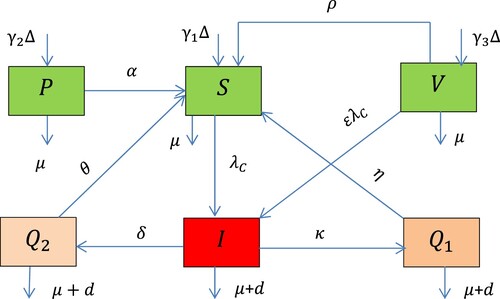
Using the COVID-19 flow diagram given in Figure 1, the dynamical system (the mathematical model) of COVID-19 transmission with vaccination, other protection measures and quarantine with treatment is six-dimensional nonlinear ordinary differential equations given by (2) $\begin{array}{rl}& {\displaystyle \frac{dS}{dt}}={\gamma }_1\mathrm{\Delta }+\alpha \mathrm{P}+\rho \mathrm{V}+\eta Q_1+\theta Q_2-\left({\lambda }_C+\mu \right)S,\\ & {\displaystyle \frac{dP}{dt}}={\gamma }_2\mathrm{\Delta }-\left(\alpha +\mu \right)P,\\ & {\displaystyle \frac{dV}{dt}}={\gamma }_3\mathrm{\Delta }-\left(\rho +\mu +ϵ{\lambda }_C\right)V,\\ & {\displaystyle \frac{dI}{dt}}={\lambda }_{C}S+ϵ{\lambda }_{C}V-\left(\mu +d+\kappa +\delta \right)I,\\ & {\displaystyle \frac{d{Q}_1}{dt}}=\kappa I-\left(\mu +d+\eta \right)Q_1,\\ & {\displaystyle \frac{d{Q}_2}{dt}}=\delta I-\left(\mu +d+\theta \right)Q_2.\end{array}$(2)

With initial conditions (3) $\begin{array}{r}S\left(0\right)>0,P\left(0\right)\ge 0,V\left(0\right)\ge 0,I\left(0\right)\ge 0,Q_1\left(0\right)\ge 0\text{ and }{Q}_2\left(0\right)\ge 0.\end{array}$(3)

The sum of all the differential equations given in (2) is (4) $\begin{array}{r}\frac{dN}{dt}=\mathrm{\Delta }-\mu N-dI-d{Q}_1-d{Q}_2.\end{array}$(4)

3. Mathematical analysis of the COVID-19 model (2)

3.1. Basic properties of the model solutions

In this section, since the system deals with human populations which cannot be negative we qualitatively analysed two basic properties of the COVID-19 model given in (2) by proving two epidemiologically crucial theorems dealing with qualitative attributes. Therefore, here we have to show that all the model variables given in Table 2 are always non-negative well as the solutions of the COVID-19 model (2) remain positive with positive initial conditions given in Equation (3) in the bounded region (5) $\begin{array}{r}\mathrm{\Omega }=\left\{\begin{array}{c}\left(S,P,V,I,Q_1,Q_2\right)\in {\mathbb{R}}_{+}^6,N\le \frac{\mathbf{\Lambda }}{\mathit{\mu }}\end{array}\right\}.\end{array}$(5) To determine the COVID-19 infection model given in (2) epidemiologically meaning full, it is fundamental to show that each model variable defined in Table 2 with positive initial conditions given in Equation (3) is nonnegative for all-time $t>0$ in the bounded region given in (5).

Theorem 3.1:

Using the initial conditions given in Equation (3) the model solutions $S\left(t\right)$, $P\left(t\right),V\left(t\right),I\left(t\right),Q_1\left(t\right),$ and $Q_2\left(t\right)$ are nonnegative for all time $t>0$ [18,25,26].

Proof:

Assume $S\left(0\right)>0$, $P\left(0\right)>0,V\left(0\right)>0$, $I\left(0\right)>0,Q_1\left(0\right)>0$, and $Q_2\left(0\right)>0$ then for all t > 0, we have to prove that $S$ (t) > 0,$P\left(t\right)>0,V\left(t\right)>0$, $I\left(t\right)>0,Q_1\left(t\right)$> 0, and $Q_2\left(t\right)$ > 0.

Define:$\tau$ = sup$\{t>0:S(\text{t})>0,P(t)>0,V(t)>0,I(t)>0,Q_1(t)>0,\text{ and }{Q}_2(t)>0\}$. Since

$S\left(t\right),P\left(t\right),V\left(t\right),I\left(t\right),Q_1\left(t\right),$ and $Q_2\left(t\right)$ are continuous we deduce that $\tau >0$. If $\tau$ = +∞, then positivity holds. But, if 0 <$\tau$ < +∞, $S\left(\tau \right)=0$ or $P\left(\tau \right)=0$ or $V\left(\tau \right)=0$ or $I\left(\tau \right)=0$ or $Q_1\left(\tau \right)=0$or$Q_2\left(\tau \right)=0.$

Now from the first equation of the model (2) we have $\frac{dS}{dt}={\gamma }_1\mathrm{\Delta }+\alpha \mathrm{P}+\rho \mathrm{V}+\eta Q_1+\theta Q_2-\left({\lambda }_C+\mu \right)S,$ and using the method of integrating factor after some calculations we have got $\begin{array}{r}S\left(\tau \right)=M_{1}S\left(0\right)+M_1{\int }_0^{\tau }ex{p}^{\int \left({\lambda }_C+\mu )\right)dt}\left({\gamma }_1\mathrm{\Delta }+\alpha \mathrm{P}+\rho \mathrm{V}+\eta Q_1+\theta Q_2\right)dt>0,\end{array}$where $M_1=ex{p}^{-\left(\mu \tau +\underset{0}{\overset{\tau }{\int }}\left({\lambda }_C\right(w)\right)}>0,S\left(0\right)>0,$ and from the definition of $\tau$ we have $\text{P}\left(t\right)>0,\text{V}\left(t\right)>0,Q_1\left(t\right)>0,$ $Q_2\left(t\right)>,$ then the solution $S\left(\tau \right)>0$ and hence $S\left(\tau \right)\ne 0$.

Again from the second equation of the model (2) we have $\frac{dP}{dt}={\gamma }_2\mathrm{\Delta }-\left(\alpha +\mu \right)P,$ and we have got $P\left(\tau \right)=M_{1}P\left(0\right)+M_1{\int }_0^{\tau }ex{p}^{\int \left(\alpha +\mu \right)dt}\left({\gamma }_2\mathrm{\Delta }\right)dt>0$where $M_1=ex{p}^{-\left(\alpha +\mu \right)\tau }>0,P\left(0\right)>0,$ and from the definition of $\tau ,$ the solution $P\left(\tau \right)>0$ hence $P\left(\tau \right)\ne 0$.

Similarly, $V\left(\tau \right)>0$ hence $V\left(\tau \right)\ne 0$, $I\left(\tau \right)>0$ hence $I\left(\tau \right)\ne 0$ $Q_1\left(\tau \right)>0$ hence $Q_1\left(\tau \right)\ne 0$, $Q_2\left(\tau \right)>0$ hence $Q_2\left(\tau \right)\ne 0$.

Thus, based on the definition, $\tau$ is not finite which means $\tau =+\mathrm{\infty }$, and hence all solutions of the COVID-19 infection model given in Equation (2) are non-negative.

Theorem 3.2:

The region $\mathrm{\Omega }$ given by Equation (5) is bounded in ${\mathbb{R}}_{+}^6$.

Proof:

Using Equation (4), since all the model variables are non-negative by Theorem 3.1, in the absence of infections, we have got $\frac{dN}{dt}\le \mathrm{\Delta }-\mu N$. Then by applying standard comparison theorem we have got $\int \frac{dN}{\mathrm{\Delta }-\mu N}\le \int dt$ and integrating both sides gives $-\frac{1}{\mu }\ln \left(\mathrm{\Delta }-\mu N\right)\le t+c$ where $c$ is some constant and after some steps of integration we have got $0\le N\left(t\right)\le \frac{\mathrm{\Delta }}{\mu }$ which means all possible model solutions with positive initial conditions given in (2) enter in the bounded region $\left(5\right)$.

3.2. Disease-free equilibrium point of the model

Disease-free equilibrium point of the COVID-19 infection model (2) is obtained by making its right-hand side as zero and setting the infected group and quarantine groups to zero as $I=Q_1=Q_2=0$ we have got $\begin{array}{rl}{S}^0& =\frac{{\gamma }_1\mathrm{\Delta }\left(\alpha +\mu \right)\left(\rho +\mu \right)+\alpha {\gamma }_2\mathrm{\Delta }\left(\rho +\mu \right)+\rho {\gamma }_3\mathrm{\Delta }\left(\alpha +\mu \right)}{\mu \left(\alpha +\mu \right)\left(\rho +\mu \right)},\\ P^0& =\frac{{\gamma }_2\mathrm{\Delta }}{\alpha +\mu },V^0=\frac{{\gamma }_3\mathrm{\Delta }}{\rho +\mu }.\end{array}$Hence the COVID-19 infection model (2) disease-free equilibrium point is given by $\begin{array}{rl}{E}_C^0& =\left(S^0,P^0,V^0,I^0,Q_1^0,Q_2^0\right)\\ & =\left(\frac{{\gamma }_1\mathrm{\Delta }\left(\alpha +\mu \right)\left(\rho +\mu \right)+\alpha {\gamma }_2\mathrm{\Delta }\left(\rho +\mu \right)+\rho {\gamma }_3\mathrm{\Delta }\left(\alpha +\mu \right)}{\mu \left(\alpha +\mu \right)\left(\rho +\mu \right)},\frac{{\gamma }_2\mathrm{\Delta }}{\alpha +\mu },\frac{{\gamma }_3\mathrm{\Delta }}{\rho +\mu },0,0,0\right).\end{array}$

3.3. Effective reproduction number of model

The effective reproduction number of COVID-19 infection measures the average number of new infections generated by one COVID-19 infectious individual in a community when some controlling strategies are in place, like protection, vaccination and quarantine with treatment. We compute the COVID-19 infection model effective reproduction number denoted by ${\mathcal{R}}_C$ using the next-generation matrix criteria specified by van den Driesch and Warmouth [29]. It is the dominant (largest) eigenvalue (spectral radius) of the matrix $F{V}^{-1}=\left[\frac{\mathrm{\partial }{\mathcal{F}}_i\left(E_C^0\right)}{\mathrm{\partial }{x}_j}\right]{\left[\frac{\mathrm{\partial }{\nu }_i\left(E_C^0\right)}{\mathrm{\partial }{x}_j}\right]}^{-1}$ where ${\mathcal{F}}_i$ is the rate of appearance of new infection in compartment $i$, ${\nu }_i$ is the transfer of infections from one compartment $i$ to another and $E_C^0$ is the COVID-19 disease-free equilibrium point. Here, after long calculations, we have got the transmission matrix given by $\begin{array}{rl}F& =\left[\begin{array}{ccc}\text{β}{S}^0+ϵ\text{β}{V}^0& 0& 0\\ 0& 0& 0\\ 0& 0& 0\end{array}\right],\end{array}$and the transition matrix given by $\begin{array}{rl}V& =\left[\begin{array}{ccc}\mu +d+\kappa +\delta & 0& 0\\ -\kappa & \mu +d+\eta & 0\\ -\delta & 0& \mu +d+\theta \end{array}\right].\end{array}$

Then using Mathematica, we have got $\begin{array}{r}{V}^{-1}=\left[\begin{array}{ccc}{\displaystyle \frac{1}{\mu +d+\kappa +\delta }}& 0& 0\\ {\displaystyle \frac{\kappa }{\left(\mu +d+\kappa +\delta \right)\left(\mu +d+\eta \right)}}& {\displaystyle \frac{1}{\left(\mu +d+\eta \right)}}& 0\\ {\displaystyle \frac{\delta }{\left(\mu +d+\kappa +\delta \right)\left(\mu +d+\theta \right)}}& 0& {\displaystyle \frac{1}{\left(\mu +d+\theta \right)}}\end{array}\right],\end{array}$and $\begin{array}{r}F{V}^{-1}=\left[\begin{array}{ccc}{\displaystyle \frac{\text{β}{S}^0+ϵ\text{β}{V}^0}{\mu +d+\kappa +\delta }}& 0& 0\\ 0& 0& 0\\ 0& 0& 0\end{array}\right].\end{array}$

The characteristic equation of the matrix $F{V}^{-1}$ is $\left|\begin{array}{cc}\frac{\text{β}{S}^0+ϵ\text{β}{V}^0}{\mu +d+\kappa +\delta }-\lambda & 0\\ 0& 0-\lambda \end{array}\right|=0$.

Then the spectral radius of the matrix $F{V}^{-1}$ (effective reproduction number ${\mathcal{R}}_C$ of the COVID-19 infection model $\left(2\right)$) is $\begin{array}{r}{\mathcal{R}}_C=\frac{\text{β}{\gamma }_1\mathrm{\Delta }\left(\alpha +\mu \right)\left(\rho +\mu \right)+\text{β}\alpha {\gamma }_2\mathrm{\Delta }\left(\rho +\mu \right)+\text{β}\rho {\gamma }_3\mathrm{\Delta }\left(\alpha +\mu \right)+\text{β}ϵ{\gamma }_3\mathrm{\Delta }\mu \left(\alpha +\mu \right)}{\mu \left(\alpha +\mu \right)\left(\rho +\mu \right)\left(\mu +d+\kappa +\delta \right)}.\end{array}$

3.4. Local stability of the model disease-free equilibrium point

Theorem 3.3:

The COVID-19 model (2) disease-free equilibrium point (DFE) denoted by $E_C^0$ is locally asymptotically stable if ${\mathcal{R}}_C<1,$ otherwise unstable.

Proof:

The local stability of the COVID-19 transmission model (2) at the disease-free equilibrium point $\begin{array}{rl}{E}_C^0& =(S^0,P^0,V^0,I^0,Q_1^0,Q_2^0)\\ & =\left(\frac{{\gamma }_1\mathrm{\Delta }\left(\alpha +\mu \right)\left(\rho +\mu \right)+\alpha {\gamma }_2\mathrm{\Delta }\left(\rho +\mu \right)+\rho {\gamma }_3\mathrm{\Delta }\left(\alpha +\mu \right)}{\mu \left(\alpha +\mu \right)\left(\rho +\mu \right)},\frac{{\gamma }_2\mathrm{\Delta }}{\alpha +\mu },\frac{{\gamma }_3\mathrm{\Delta }}{\rho +\mu },0,0,0\right)\end{array}$can be analysed using Routh–Hurwitz local stability criteria stated in Theorem 3.1 of [27].

The Jacobian matrix of the COVID-19 dynamical system (2) at the given disease-free equilibrium point is given by $\begin{array}{r}J\left(E_C^0\right)=\left(\begin{array}{cccccc}-\mu & \alpha & \rho & 0& \eta & \theta \\ 0& -\left(\alpha +\mu \right)& 0& 0& 0& 0\\ 0& 0& -\left(\rho +\mu \right)& -ϵ\text{β}{V}^0& 0& 0\\ 0& 0& 0& D& 0& 0\\ 0& 0& 0& \kappa & -\left(\mu +d+\eta \right)& 0\\ 0& 0& 0& 0& \delta & -\left(\mu +d+\theta \right)\end{array}\right),\end{array}$where $D=\text{β}{S}^0+ϵ\text{β}{V}^0-\left(\mu +d+\kappa +\delta \right).$

Then the characteristic equation of the Jacobian matrix $J\left(E_C^0\right)$ is given by $\begin{array}{rl}& |\begin{array}{ccc}-\mu -\lambda & \alpha & \rho \\ 0& -\left(\alpha +\mu \right)-\lambda & 0\\ -ϵ\text{β}{V}^0& 0& 0\\ M-\lambda & 0& 0\\ \kappa & -\left(\mu +d+\eta \right)-\lambda & 0\\ 0& \delta & -\left(\mu +d+\theta \right)-\lambda \end{array}\\ & \begin{array}{ccc}0& \eta & \theta \\ 0& 0& 0\\ -ϵ\text{β}{V}^0& 0& 0\\ M-\lambda & 0& 0\\ \kappa & -\left(\mu +d+\eta \right)-\lambda & 0\\ 0& \delta & -\left(\mu +d+\theta \right)-\lambda \end{array}|=0,\end{array}$where $M=\text{β}{S}^0+ϵ\text{β}{V}^0-\left(\mu +d+\kappa +\delta \right)$ and after some steps of computations we have got${\lambda }_1=-\mu <0$ or ${\lambda }_2=-\left(\alpha +\mu \right)<0$ or ${\lambda }_3=-\left(\rho +\mu \right)<0$ or ${\lambda }_4=\left(\mu +d+\kappa +\delta \right)\left[{\mathcal{R}}_C-1\right]<0$ if ${\mathcal{R}}_C<1$ or ${\lambda }_5=-\left(\mu +d+\eta \right)<0$ or ${\lambda }_5=-\left(\mu +d+\theta \right)<0$.

Hence, since all the eigenvalues of the characteristics polynomials of Jacobian matrix $J\left(E_C^0\right)$ for the COVID-19 model given in Equation (2) are negative if ${\mathcal{R}}_C<1$ the DFE is locally asymptotically stable. Here the biological implication of Theorem 3.3 is that the COVID-19 diseases can be eradicated from the population (when the threshold quantity ${\mathcal{R}}_C<1$) if the initial sizes of the population of the COVID-19 infection are in the basin of attraction of the disease-free equilibrium ($E_C^0$). Therefore, a small change of COVID-19 infected individuals into the population will not generate large outbreaks of the diseases, and the diseases will eradicate from the community over time.

3.5. Existence of endemic equilibrium point (s) of the model

In this section, before justifying the global stability of the COVID-19 infection model (2) DFE point, it is crucial to examine the number of equilibrium point(s).

Let $E_C^{\ast }=\left(S^{\ast },P^{\ast },V^{\ast },I^{\ast },Q_1^{\ast },Q_2^{\ast }\right)$ be the corresponding arbitrary endemic equilibrium point of the COVID-19 infection model (2) and ${\lambda }_C^{\ast }=\text{β}{I}^{\ast }$ be the COVID-19 mass action incidence rate (‘force of infection’) at $E_C^{\ast }$. To find the equilibrium point(s) for which COVID-19 infection is endemic in the population, Equation (2) is solved in terms of ${\lambda }_C^{\ast }=\text{β}{I}^{\ast }$. The endemic equilibrium point(s) of the model are obtained by making system (2) equal to zero as $\begin{array}{rl}& {\gamma }_2\mathrm{\Delta }-\left(\alpha +\mu \right)P=0,\end{array}$ $\begin{array}{rl}& \Rightarrow P^{\ast }=\frac{{\gamma }_2\mathrm{\Delta }}{\alpha +\mu }.\end{array}$ $\begin{array}{rl}& {\gamma }_3\mathrm{\Delta }-\left(\rho +\mu +ϵ{\lambda }_C\right)V=0,\end{array}$ $\begin{array}{rl}& \Rightarrow V^{\ast }=\frac{{\gamma }_3\mathrm{\Delta }}{\rho +\mu +ϵ{\lambda }_C^{\ast }}.\end{array}$ $\begin{array}{rl}& {\lambda }_{C}S+ϵ{\lambda }_{C}V-\left(\mu +d+\kappa +\delta \right)I=0,\end{array}$ $\begin{array}{rl}& \Rightarrow S^{\ast }=\frac{\left(\mu +d+\kappa +\delta \right)\left(\rho +\mu +ϵ{\lambda }_C^{\ast }\right)I-ϵ{\lambda }_C^{\ast }{\gamma }_3\mathrm{\Delta }}{{\lambda }_C^{\ast }\left(\rho +\mu +ϵ{\lambda }_C^{\ast }\right)}.\end{array}$ $\begin{array}{rl}& \kappa I-\left(\mu +d+\eta \right)Q_1=0,\end{array}$ $\begin{array}{rl}& \Rightarrow Q_1^{\ast }=\frac{\kappa I}{\left(\mu +d+\eta \right)}.\end{array}$ $\begin{array}{rl}& \delta I-\left(\mu +d+\theta \right)Q_2=0,\end{array}$ $\begin{array}{rl}& \Rightarrow Q_2^{\ast }=\frac{\delta I}{\left(\mu +d+\theta \right)}.\end{array}$

Then by substituting all-star in the first equation of system (2), we have $\begin{array}{rl}{\gamma }_1\mathrm{\Delta }& +\alpha \mathrm{P}+\rho \mathrm{V}+\eta Q_1+\theta Q_2-\left({\lambda }_C+\mu \right)S=0.\end{array}$ $\begin{array}{rl}& \Rightarrow {\gamma }_1\mathrm{\Delta }+\frac{\alpha {\gamma }_2\mathrm{\Delta }}{\alpha +\mu }+\frac{\rho {\gamma }_3\mathrm{\Delta }}{\rho +\mu +ϵ{\lambda }_C^{\ast }}+\frac{\eta \kappa I}{\left(\mu +d+\eta \right)}+\frac{\theta \delta I}{\left(\mu +d+\theta \right)}\\ & -\left({\lambda }_C+\mu \right)\frac{\left(\mu +d+\kappa +\delta \right)\left(\rho +\mu +ϵ{\lambda }_C^{\ast }\right)I-ϵ{\lambda }_C^{\ast }{\gamma }_3\mathrm{\Delta }}{{\lambda }_C^{\ast }\left(\rho +\mu +ϵ{\lambda }_C^{\ast }\right)}=0.\end{array}$ $\begin{array}{rl}& \Rightarrow {\gamma }_1\mathrm{\Delta }+\frac{\alpha {\gamma }_2\mathrm{\Delta }}{\alpha +\mu }+\frac{\rho {\gamma }_3\mathrm{\Delta }}{\rho +\mu +ϵ{\lambda }_C^{\ast }}+\frac{\eta \kappa I}{\left(\mu +d+\eta \right)}+\frac{\theta \delta I}{\left(\mu +d+\theta \right)}\\ & +\frac{ϵ{\lambda }_C^{\ast }{\gamma }_3\mathrm{\Delta }\left({\lambda }_C^{\ast }+\mu \right)}{{\lambda }_C^{\ast }\left(\rho +\mu +ϵ{\lambda }_C^{\ast }\right)}-\frac{\left({\lambda }_C^{\ast }+\mu \right)\left(\mu +d+\kappa +\delta \right)\left(\rho +\mu +ϵ{\lambda }_C^{\ast }\right)I}{{\lambda }_C^{\ast }\left(\rho +\mu +ϵ{\lambda }_C^{\ast }\right)}=0.\end{array}$ $\begin{array}{rl}& \Rightarrow {\gamma }_1\mathrm{\Delta }+\frac{\alpha {\gamma }_2\mathrm{\Delta }}{\alpha +\mu }+\frac{\rho {\gamma }_3\mathrm{\Delta }}{\rho +\mu +ϵ{\lambda }_C^{\ast }}+\frac{ϵ{\lambda }_C^{\ast }{\gamma }_3\mathrm{\Delta }\left({\lambda }_C^{\ast }+\mu \right)}{{\lambda }_C^{\ast }\left(\rho +\mu +ϵ{\lambda }_C^{\ast }\right)}\\ & -[\frac{\left({\lambda }_C^{\ast }+\mu \right)\left(\mu +d+\kappa +\delta \right)\left(\rho +\mu +ϵ{\lambda }_C^{\ast }\right)}{{\lambda }_C^{\ast }\left(\rho +\mu +ϵ{\lambda }_C^{\ast }\right)}-\frac{\eta \kappa }{\left(\mu +d+\eta \right)}\\ & -\frac{\theta \delta }{\left(\mu +d+\theta \right)}]I=0.\end{array}$ $\begin{array}{rl}& \Rightarrow {\gamma }_1\mathrm{\Delta }+\frac{\alpha {\gamma }_2\mathrm{\Delta }}{\alpha +\mu }+\frac{\rho {\gamma }_3\mathrm{\Delta }}{\rho +\mu +ϵ{\lambda }_C^{\ast }}+\frac{ϵ{\lambda }_C^{\ast }{\gamma }_3\mathrm{\Delta }\left({\lambda }_C^{\ast }+\mu \right)}{{\lambda }_C^{\ast }\left(\rho +\mu +ϵ{\lambda }_C^{\ast }\right)}-\\ & \left[\frac{\begin{array}{c}\left({\lambda }_C^{\ast }+\mu \right)\left(\mu +d+\kappa +\delta \right)\left(\rho +\mu +ϵ{\lambda }_C^{\ast }\right)\left(\mu +d+\eta \right)\left(\mu +d+\theta \right)\\ -\eta \kappa {\lambda }_C^{\ast }\left(\rho +\mu +ϵ{\lambda }_C^{\ast }\right)\left(\mu +d+\theta \right)-\theta \delta {\lambda }_C^{\ast }\left(\rho +\mu +ϵ{\lambda }_C^{\ast }\right)\left(\mu +d+\eta \right)\end{array}}{{\lambda }_C^{\ast }\left(\rho +\mu +ϵ{\lambda }_C^{\ast }\right)\left(\mu +d+\eta \right)\left(\mu +d+\theta \right)}\right]I=0.\end{array}$ $\begin{array}{rl}\Rightarrow I^{\ast }& =\frac{m_1{\lambda }_C^{\ast }\left(\rho +\mu +ϵ{\lambda }_C^{\ast }\right)+m_2{\lambda }_C^{\ast }+m_3{\lambda }_C^{\ast }\left({\lambda }_C^{\ast }+\mu \right)}{\left(\rho +\mu +ϵ{\lambda }_C^{\ast }\right)\left[m_4\left({\lambda }_C^{\ast }+\mu \right)-m_5{\lambda }_C^{\ast }\right]}.\end{array}$

where $\begin{array}{rl}{m}_1& ={\gamma }_1\mathrm{\Delta }\left(\alpha +\mu \right)\left(\mu +d+\eta \right)\left(\mu +d+\theta \right)+\alpha {\gamma }_2\mathrm{\Delta }\left(\mu +d+\eta \right)\left(\mu +d+\theta \right).\end{array}$ $\begin{array}{rl}{m}_2& =\rho {\gamma }_3\mathrm{\Delta }\left(\alpha +\mu \right)\left(\mu +d+\eta \right)\left(\mu +d+\theta \right).\end{array}$ $\begin{array}{rl}{m}_3& =ϵ{\gamma }_3\mathrm{\Delta }\left(\alpha +\mu \right)\left(\mu +d+\eta \right)\left(\mu +d+\theta \right).\end{array}$ $\begin{array}{rl}{m}_4& =\left(\mu +d+\kappa +\delta \right)\left(\mu +d+\eta \right)\left(\mu +d+\theta \right)\left(\alpha +\mu \right).\end{array}$ $\begin{array}{rl}{m}_5& =\eta \kappa \left(\mu +d+\theta \right)\left(\alpha +\mu \right)+\theta \delta \left(\mu +d+\eta \right)\left(\alpha +\mu \right).\end{array}$

Then the remaining state variables will be obtained by substituting $I^{\ast }$ as $\begin{array}{rl}{P}^{\ast }& =\frac{{\gamma }_2\mathrm{\Delta }}{\alpha +\mu },\end{array}$ $\begin{array}{rl}{V}^{\ast }& =\frac{{\gamma }_3\mathrm{\Delta }}{\rho +\mu +ϵ{\lambda }_C^{\ast }},\end{array}$ $\begin{array}{rl}{S}^{\ast }& =\frac{\begin{array}{c}\left(\mu +d+\kappa +\delta \right)\left[m_1{\lambda }_C^{\ast }\right(\rho +\mu +ϵ{\lambda }_C^{\ast })+m_2{\lambda }_C^{\ast }\\ +m_3{\lambda }_C^{\ast }\left({\lambda }_C^{\ast }+\mu \right)]-ϵ{\lambda }_C^{\ast }{\gamma }_3\mathrm{\Delta }[m_4\left({\lambda }_C^{\ast }+\mu \right)-m_5{\lambda }_C^{\ast }]\end{array}}{{\lambda }_C^{\ast }\left(\rho +\mu +ϵ{\lambda }_C^{\ast }\right)\left[m_4\left({\lambda }_C^{\ast }+\mu \right)-m_5{\lambda }_C^{\ast }\right]},\end{array}$ $\begin{array}{rl}{Q}_1^{\ast }& =\frac{m_1\kappa {\lambda }_C^{\ast }\left(\rho +\mu +ϵ{\lambda }_C^{\ast }\right)+m_2\kappa {\lambda }_C^{\ast }+m_3{\lambda }_C^{\ast }\left({\lambda }_C^{\ast }+\mu \right)}{\left(\mu +d+\eta \right)\left(\rho +\mu +ϵ{\lambda }_C^{\ast }\right)\left[m_4\left({\lambda }_C^{\ast }+\mu \right)-m_5{\lambda }_C^{\ast }\right]},\end{array}$ $\begin{array}{rl}{Q}_2^{\ast }& =\frac{m_1\delta {\lambda }_C^{\ast }\left(\rho +\mu +ϵ{\lambda }_C^{\ast }\right)+m_2\delta {\lambda }_C^{\ast }+m_3{\lambda }_C^{\ast }\left({\lambda }_C^{\ast }+\mu \right)}{\left(\mu +d+\theta \right)\left(\rho +\mu +ϵ{\lambda }_C^{\ast }\right)\left[m_4\left({\lambda }_C^{\ast }+\mu \right)-m_5{\lambda }_C^{\ast }\right]}.\end{array}$

Now substituting $I^{\ast }$ into the COVID-19 force of infection ${\lambda }_C^{\ast }=\text{β}{I}^{\ast }$ given in Equation (1), we have obtained that ${\lambda }_C^{\ast }=\frac{\text{β}{m}_1{\lambda }_C^{\ast }\left(\rho +\mu +ϵ{\lambda }_C^{\ast }\right)+\text{β}{m}_2{\lambda }_C^{\ast }+\text{β}{m}_3{\lambda }_C^{\ast }\left({\lambda }_C^{\ast }+\mu \right)}{\left(\rho +\mu +ϵ{\lambda }_C^{\ast }\right)\left[m_4\left({\lambda }_C^{\ast }+\mu \right)-m_5{\lambda }_C^{\ast }\right]}$. $\begin{array}{rl}& \Rightarrow {\lambda }_C^{\ast }\left(\rho +\mu +ϵ{\lambda }_C^{\ast }\right)\left[m_4\left({\lambda }_C^{\ast }+\mu \right)-m_5{\lambda }_C^{\ast }\right]=\text{β}{m}_1{\lambda }_C^{\ast }\left(\rho +\mu +ϵ{\lambda }_C^{\ast }\right)+\text{β}{m}_2{\lambda }_C^{\ast }\\ & +\text{β}{m}_3{\lambda }_C^{\ast }\left({\lambda }_C^{\ast }+\mu \right)\end{array}$ $\begin{array}{rl}& \left(\rho +\mu +ϵ{\lambda }_C^{\ast }\right)\left[m_4\left({\lambda }_C^{\ast }+\mu \right)-m_5{\lambda }_C^{\ast }\right]=\text{β}{m}_1\left(\rho +\mu +ϵ{\lambda }_C^{\ast }\right)+\text{β}{m}_2+\text{β}{m}_3\left({\lambda }_C^{\ast }+\mu \right)\end{array}$ $\begin{array}{rl}& m_4\left({\lambda }_C^{\ast }+\mu \right)\left(\rho +\mu \right)+m_4\left({\lambda }_C^{\ast }+\mu \right)ϵ{\lambda }_C^{\ast }-m_5{\lambda }_C^{\ast }\left(\rho +\mu \right)-m_5{\lambda }_C^{\ast }ϵ{\lambda }_C^{\ast }\\ & =\text{β}{m}_1\left(\rho +\mu \right)+\text{β}{m}_1ϵ{\lambda }_C^{\ast }+\text{β}{m}_2+\mu \text{β}{m}_3+\text{β}{m}_3{\lambda }_C^{\ast }\end{array}$ $\begin{array}{rl}& m_4\left(\rho +\mu \right){\lambda }_C^{\ast }+m_4\mu \left(\rho +\mu \right)+m_4ϵ{\lambda }_C^{\ast }{\lambda }_C^{\ast }+\mu m_4ϵ{\lambda }_C^{\ast }-m_5{\lambda }_C^{\ast }\left(\rho +\mu \right)-m_5{\lambda }_C^{\ast }ϵ{\lambda }_C^{\ast }\\ & =\text{β}{m}_1\left(\rho +\mu \right)+\text{β}{m}_1ϵ{\lambda }_C^{\ast }+\text{β}{m}_2+\mu \text{β}{m}_3+\text{β}{m}_3{\lambda }_C^{\ast }\end{array}$ $\begin{array}{rl}& m_4\left(\rho +\mu \right){\lambda }_C^{\ast }+m_4\mu \left(\rho +\mu \right)+m_4ϵ\lambda {}_C^{\ast 2}+\mu m_4ϵ{\lambda }_C^{\ast }-m_5{\lambda }_C^{\ast }\left(\rho +\mu \right)-m_5ϵ\lambda {}_C^{\ast 2}\\ & =\text{β}{m}_1\left(\rho +\mu \right)+\text{β}{m}_1ϵ{\lambda }_C^{\ast }+\text{β}{m}_2+\mu \text{β}{m}_3+\text{β}{m}_3{\lambda }_C^{\ast }\\ & \left[m_4ϵ-m_5ϵ\right]\lambda {}_C^{\ast 2}+\left[m_4\left(\rho +\mu \right)+\mu m_4ϵ-m_5\left(\rho +\mu \right)-\text{β}{m}_1ϵ-\text{β}{m}_3\right]{\lambda }_C^{\ast }\\ & +\left(\rho +\mu \right)\left(m_4\mu -\text{β}{m}_1\right)-\text{β}\left(m_2+\mu m_3\right)=0.\end{array}$ (6) $\begin{array}{rl}& \Rightarrow a_2\lambda {}_C^{\ast 2}+a_1{\lambda }_C^{\ast }+a_0=0.\end{array}$(6) The coefficients of Equation (6) are given by $\begin{array}{rl}{a}_2& =ϵ\left[m_4-m_5\right]>0,\end{array}$ $\begin{array}{rl}{a}_1& =m_4\left(\rho +\mu \right)+\mu m_4ϵ-m_5\left(\rho +\mu \right)-\text{β}{m}_1ϵ-\text{β}{m}_3,\end{array}$ $\begin{array}{rl}{a}_0& =m_4\mu \left(\rho +\mu \right)-\text{β}\left(m_1\left(\rho +\mu \right)+m_2+\mu m_3\right),\end{array}$ $\begin{array}{rl}& =\left(\mu +d+\kappa +\delta \right)\left(\mu +d+\eta \right)\left(\mu +d+\theta \right)\left(\alpha +\mu \right)\mu \left(\rho +\mu \right)\left(1-{\mathcal{R}}_C\right),\end{array}$where ${\mathcal{R}}_C=\frac{\text{β}\left(\left[{\gamma }_1\mathrm{\Delta }\left(\alpha +\mu \right)+\alpha {\gamma }_2\mathrm{\Delta }\right]\left(\rho +\mu \right)+\rho {\gamma }_3\mathrm{\Delta }\left(\alpha +\mu \right)+\mu ϵ{\gamma }_3\mathrm{\Delta }\left(\alpha +\mu \right)\right)}{\left(\mu +d+\kappa +\delta \right)\left(\alpha +\mu \right)\mu \left(\rho +\mu \right)}$.

It can be seen that $a_2>0$ (since all the model parameters described in Table 1 are nonnegative). Moreover, $a_0>0$ whenever ${\mathcal{R}}_C<1$. Thus the number of possible positive real roots the polynomial (6) can have depends on the signs of $a_2,a_1$ and $a_0$. This can be examined through the use of Descartes’ rule of signs on the quadratic polynomial $f\left(x\right)$  = $a_2{x}^2+a_{1}x+a_0$ (with $x$ = ${\lambda }_C^{\ast }$). Hence, we establish the following results.

Theorem 3.4:

The COVID-19 infection model (2)

1. has a unique endemic equilibrium point if ${\mathcal{R}}_C>1$ and $a_1<0$.

2. could have two endemic equilibrium points if ${\mathcal{R}}_C<1$ and $a_1<0$.

Here, the expression given in (b) shows that the existence of backward bifurcation in the COVID-19 model (2), i.e. the locally asymptotically stable disease-free equilibrium point co-exists with a locally asymptotically stable endemic equilibrium point if ${\mathcal{R}}_C<1$; examples of the exhibit of backward bifurcation phenomenon in deterministic and compartmental epidemiological models discussed in [3,13,18,24,26]. Biologically the classical need of having the COVID-19 reproduction number ${\mathcal{R}}_C$ be less than 1, although necessary, is not sufficient for the complete control of the COVID-19 disease. In the next Section 3.6, we will explore the existence of the backward bifurcation phenomenon in the COVID-19 model (2).

3.6. Backward bifurcation analysis of the model

For the biological interpretation of the COVID-19 infection, it is fundamental to determine and classify the type of bifurcation the COVID-19 model (2) may exhibit. The biological aspect of the phenomenon of backward bifurcation is that the classical epidemiological need of having the effective reproduction number of COVID-19 infection, ${\mathcal{R}}_C$ be less than unity, even if it is a necessity, it is not sufficient to eradicate the COVID-19 infection from the considered community. In other words, the backward bifurcation property of the model (2) makes the complete control of COVID-19 in the population very complicated.

Theorem 3.5:

The COVID-19 model given in (2) exhibits backward bifurcation at ${\mathcal{R}}_C=1$ whenever $L>K$ holds where $L=\frac{\text{β}\eta \kappa }{\left(\mu +d+\eta \right)\mu }+\frac{\text{β}\theta \delta }{\left(\mu +d+\theta \right)\mu }$ and $K=\frac{\text{β}{\text{β}}^{\ast }\rho ϵx_3^0}{\left(\rho +\mu \right)\mu }+\frac{{\text{β}}^{\ast }{x}_1^0}{\mu }+\frac{\text{β}ϵ{\text{β}}^{\ast }ϵx_3^0}{\left(\rho +\mu \right)}.$

Proof:

Let $E_C^{\ast }=\left(S^{\ast },P^{\ast },V^{\ast },I^{\ast },Q_1^{\ast },Q_2^{\ast }\right)$ represents any arbitrary endemic equilibrium of the COVID-19 infection model (2) (i.e., an endemic equilibrium in which at least one of the infected components is non-zero). The existence of backward bifurcation will be analysed using the version of Centre Manifold Theory [4]. To apply this theory, it is necessary to carry out the following change of variables.

Suppose $S=x_1$, $P=x_2,V=x_3,I=x_4,Q_1=x_5$, and $Q_2=x_6$ so that $N=x_1+x_2+x_3+x_4+x_5+x_6$. Furthermore, by using vector notation $X=(x_1,x_2,x_3,x_4,x_5,x_6{)}^T$, the COVID-19 infection model (2) can be written in the form $\frac{dX}{dt}=F\left(X\right)$ with

$F=(f_1,f_2,f_3,f_4,f_5,f_6{)}^T$, as follows: (7) $\begin{array}{r}\begin{array}{l}{\displaystyle \frac{d{x}_1}{dt}}={\gamma }_1\mathrm{\Delta }+\alpha x_2+\rho x_3+\eta x_5+\theta x_6-\left({\lambda }_C+\mu \right)x_1,\\ {\displaystyle \frac{d{x}_2}{dt}}={\gamma }_2\mathrm{\Delta }-\left(\alpha +\mu \right)x_2,\\ {\displaystyle \frac{d{x}_3}{dt}}={\gamma }_3\mathrm{\Delta }-\left(\rho +\mu +ϵ{\lambda }_C\right)x_3,\\ {\displaystyle \frac{d{x}_4}{dt}}={\lambda }_C{x}_1+ϵ{\lambda }_C{x}_3-\left(\mu +d+\kappa +\delta \right)x_4,\\ {\displaystyle \frac{d{x}_5}{dt}}=\kappa x_4-\left(\mu +d+\eta \right)x_5,\\ {\displaystyle \frac{d{x}_6}{dt}}=\delta x_4-\left(\mu +d+\theta \right)x_6.\end{array}\end{array}$(7) where ${\lambda }_C=\text{β}{x}_4$.

Then the Jacobian matrix of the system given in Equation (7) at the DFE point $E_C^0$, denoted by $J\left(E_C^0\right)$ is given by $\begin{array}{r}J\left(E_C^0\right)=\left(\begin{array}{cccccc}-\mu & \alpha & \rho & -\text{β}{x}_1^0& \eta & \theta \\ 0& -\left(\alpha +\mu \right)& 0& 0& 0& 0\\ 0& 0& -\left(\rho +\mu \right)& -\text{β}ϵx_3^0& 0& 0\\ 0& 0& 0& A& 0& 0\\ 0& 0& 0& \kappa & -\left(\mu +d+\eta \right)& 0\\ 0& 0& 0& \delta & 0& -\left(\mu +d+\theta \right)\end{array}\right),\end{array}$where $A=\text{β}{x}_1^0+\text{β}ϵx_3^0-\left(\mu +d+\kappa +\delta \right)$.

Now let us consider, ${\mathcal{R}}_C=1$ and suppose that $\text{β}$ $={\text{β}}^{\ast }$ is chosen as a bifurcation parameter.

From ${\mathcal{R}}_C=1$, we have that $\begin{array}{r}{\mathcal{R}}_C=\frac{\text{β}{\gamma }_1\mathrm{\Delta }\left(\alpha +\mu \right)\left(\rho +\mu \right)+\text{β}\alpha {\gamma }_2\mathrm{\Delta }\left(\rho +\mu \right)+\text{β}\rho {\gamma }_3\mathrm{\Delta }\left(\alpha +\mu \right)+\text{β}ϵ{\gamma }_3\mathrm{\Delta }\left(\alpha +\mu \right)}{\mu \left(\alpha +\mu \right)\left(\rho +\mu \right)\left(\mu +d+\kappa +\delta \right)}=1.\end{array}$

And solving for $\text{β}$, we have got $\begin{array}{r}\text{β}={\text{β}}^{\ast }=\frac{\mu \left(\alpha +\mu \right)\left(\rho +\mu \right)\left(\mu +d+\kappa +\delta \right)}{{\gamma }_1\mathrm{\Delta }\left(\alpha +\mu \right)\left(\rho +\mu \right)+\alpha {\gamma }_2\mathrm{\Delta }\left(\rho +\mu \right)+\rho {\gamma }_3\mathrm{\Delta }\left(\alpha +\mu \right)+ϵ{\gamma }_3\mathrm{\Delta }{\gamma }_1\mathrm{\Delta }\left(\alpha +\mu \right)}.\end{array}$

Then $\begin{array}{r}{J}_{{\text{β}}^{\ast }}=\left(\begin{array}{cccccc}-\mu & \alpha & \rho & -{\text{β}}^{\ast }{x}_1^0& \eta & \theta \\ 0& -\left(\alpha +\mu \right)& 0& 0& 0& 0\\ 0& 0& -\left(\rho +\mu \right)& -{\text{β}}^{\ast }ϵx_3^0& 0& 0\\ 0& 0& 0& B& 0& 0\\ 0& 0& 0& \kappa & -\left(\mu +d+\eta \right)& 0\\ 0& 0& 0& \delta & 0& -\left(\mu +d+\theta \right)\end{array}\right),\end{array}$where $B={\text{β}}^{\ast }{x}_1^0+{\text{β}}^{\ast }ϵx_3^0-\left(\mu +d+\kappa +\delta \right)$.

After some steps of the calculations, the eigenvalues of $J_{{\text{β}}^{\ast }}$ are given by ${\lambda }_1=-\mu$ or ${\lambda }_2=-\left(\alpha +\mu \right)$ or ${\lambda }_3=-\left(\rho +\mu \right)$ or ${\lambda }_4=0$ or ${\lambda }_5=-\left(\mu +d+\eta \right)$ or ${\lambda }_6=-\left(\mu +d+\theta \right)$.

Here the Jacobian matrix $J\left(E_C^0\right)$ of Equation (7) at the DFE point such that $\text{β}={\text{β}}^{\ast }$, denoted by $J_{{\text{β}}^{\ast }}$, has a single zero eigenvalue with all the other eigenvalues having negative real part. Thus, based on the version of Centre Manifold theory approach given by Theorem 3.2 of Castillo–Chavez and Song [4] we can analyse the COVID-19 model (2) undergoes backward bifurcation at ${\mathcal{R}}_C=1$.

The two types of eigenvectors of the matrix $J_{{\text{β}}^{\ast }}$ for the case ${\mathcal{R}}_C=1$ of the system (7) at $\text{β}={\text{β}}^{\ast }$ are the right eigenvectors and the left eigenvectors.

Then the right eigenvectors associated with the zero eigenvalues given by $u=(u_1,u_2,u_3,u_4,u_5,u_6{)}^T$ are determined as (8) $\begin{array}{rl}& \left(\begin{array}{cccccc}-\mu & \alpha & \rho & -{\text{β}}^{\ast }{x}_1^0& \eta & \theta \\ 0& -\left(\alpha +\mu \right)& 0& 0& 0& 0\\ 0& 0& -\left(\rho +\mu \right)& -{\text{β}}^{\ast }ϵx_3^0& 0& 0\\ 0& 0& 0& B& 0& 0\\ 0& 0& 0& \kappa & -\left(\mu +d+\eta \right)& 0\\ 0& 0& 0& \delta & 0& -\left(\mu +d+\theta \right)\end{array}\right)\\ & \times \left(\begin{array}{c}{u}_1\\ u_2\\ u_3\\ u_4\\ u_5\\ u_6\end{array}\right)=\left(\begin{array}{c}0\\ 0\\ 0\\ 0\\ 0\\ 0\end{array}\right).\end{array}$(8) Therefore, solving Equation (8) the right eigenvectors associated with the zero eigenvalue are given by $\begin{array}{rl}{u}_1& =\left[\frac{\eta \kappa }{\left(\mu +d+\eta \right)\mu }+\frac{\theta \delta }{\left(\mu +d+\theta \right)\mu }-\frac{{\text{β}}^{\ast }\rho ϵx_3^0}{\left(\rho +\mu \right)\mu }-\frac{{\text{β}}^{\ast }{x}_1^0}{\mu }\right]u_4,\end{array}$ $\begin{array}{rl}{u}_2& =0,\end{array}$ $\begin{array}{rl}{u}_3& =-\frac{{\text{β}}^{\ast }ϵx_3^0}{\left(\rho +\mu \right)}{u}_4<0,\end{array}$ $\begin{array}{rl}{u}_4& =u_4>0,\end{array}$ $\begin{array}{rl}{u}_5& =\frac{\kappa }{\left(\mu +d+\eta \right)}{u}_4>0,\end{array}$ $\begin{array}{rl}{u}_6& =\frac{\delta }{\left(\mu +d+\theta \right)}{u}_4>0.\end{array}$

Similarly, the left eigenvector associated with the zero eigenvalues given by $v=(v_1,v_2,v_3,v_4,v_5,v_6{)}^T$ are determined as (9) $\begin{array}{rl}& {\left(\begin{array}{c}{v}_1\\ v_2\\ v_3\\ v_4\\ v_5\\ v_6\end{array}\right)}^T\left(\begin{array}{cccccc}-\mu & \alpha & \rho & -{\text{β}}^{\ast }{x}_1^0& \eta & \theta \\ 0& -\left(\alpha +\mu \right)& 0& 0& 0& 0\\ 0& 0& -\left(\rho +\mu \right)& -{\text{β}}^{\ast }ϵx_3^0& 0& 0\\ 0& 0& 0& B& 0& 0\\ 0& 0& 0& \kappa & -\left(\mu +d+\eta \right)& 0\\ 0& 0& 0& \delta & 0& -\left(\mu +d+\theta \right)\end{array}\right)\\ & =\left(\begin{array}{c}0\\ 0\\ 0\\ 0\\ 0\\ 0\end{array}\right).\end{array}$(9) Then solving Equation (9), the left eigenvectors associated with the zero eigenvalue are given by $\begin{array}{r}{v}_1=v_2=v_3=v_5=v_6=0\text{and}{v}_4=v_4>0.\end{array}$

Now applying the theory of partial derivatives the non-zero second order partial derivatives at the disease-free equilibrium point ${\xi }^0=\left(x_1^0,x_2^0,x_3^0,x_4^0,x_5^0,x_6^0\right)=\left(\frac{{\gamma }_1\mathrm{\Delta }\left(\alpha +\mu \right)\left(\rho +\mu \right)+\alpha {\gamma }_2\mathrm{\Delta }\left(\rho +\mu \right)+\rho {\gamma }_3\mathrm{\Delta }\left(\alpha +\mu \right)}{\mu \left(\alpha +\mu \right)\left(\rho +\mu \right)},\frac{{\gamma }_2\mathrm{\Delta }}{\alpha +\mu },\frac{{\gamma }_3\mathrm{\Delta }}{\rho +\mu },0,0,0\right)$ of the system (7) are given by $\begin{array}{rl}\frac{{\mathrm{\partial }}^2{f}_4}{\mathrm{\partial }{x}_1\mathrm{\partial }{x}_4}& =2\text{β},\end{array}$ $\begin{array}{rl}\frac{{\mathrm{\partial }}^2{f}_4}{\mathrm{\partial }{x}_3\mathrm{\partial }{x}_4}& =2\text{β}ϵ,\end{array}$ $\begin{array}{rl}\frac{{\mathrm{\partial }}^2{f}_4}{\mathrm{\partial }{x}_4\mathrm{\partial }\text{β}}& =x_1^0+ϵx_3^0.\end{array}$

Thus the bifurcation coefficients $a$ and $b$ are determined as (10) $\begin{array}{rl}a& ={\sum }_{i,j}^6{v}_4{u}_i{u}_j\frac{{\mathrm{\partial }}^2{f}_4}{\mathrm{\partial }{x}_i\mathrm{\partial }{x}_j}=2v_4{u}_1{u}_4\frac{{\mathrm{\partial }}^2{f}_4}{\mathrm{\partial }{x}_1\mathrm{\partial }{x}_4}+2v_4{u}_3{u}_4\frac{{\mathrm{\partial }}^2{f}_4}{\mathrm{\partial }{x}_3\mathrm{\partial }{x}_4},\\ & 2v_4{u}_4\left[u_1\frac{{\mathrm{\partial }}^2{f}_4}{\mathrm{\partial }{x}_1\mathrm{\partial }{x}_4}+u_3\frac{{\mathrm{\partial }}^2{f}_4}{\mathrm{\partial }{x}_3\mathrm{\partial }{x}_4}\right],\\ & 2v_4{u_4}^2\left[\frac{\text{β}\eta \kappa }{\left(\mu +d+\eta \right)\mu }+\frac{\text{β}\theta \delta }{\left(\mu +d+\theta \right)\mu }-\frac{\text{β}{\text{β}}^{\ast }\rho ϵx_3^0}{\left(\rho +\mu \right)\mu }-\frac{{\text{β}}^{\ast }{x}_1^0}{\mu }-\frac{\text{β}ϵ{\text{β}}^{\ast }ϵx_3^0}{\left(\rho +\mu \right)}\right],\\ & =2v_4{u_4}^2\left[L-K\right]\text{where}L=\frac{\text{β}\eta \kappa }{\left(\mu +d+\eta \right)\mu }+\frac{\text{β}\theta \delta }{\left(\mu +d+\theta \right)\mu }\\ \text{where}& =\frac{\text{β}{\text{β}}^{\ast }\rho ϵx_3^0}{\left(\rho +\mu \right)\mu }+\frac{{\text{β}}^{\ast }{x}_1^0}{\mu }+\frac{\text{β}ϵ{\text{β}}^{\ast }ϵx_3^0}{\left(\rho +\mu \right)}.\end{array}$(10) $\begin{array}{rl}b& ={\sum }_{i,k=1}^6{v}_k{u}_i\frac{{\mathrm{\partial }}^2{f}_k}{\mathrm{\partial }{x}_i\mathrm{\partial }\text{β}}\left(E_C^0\right)={\sum }_{i=1}^6{v}_4{u}_i\frac{{\mathrm{\partial }}^2{f}_4}{\mathrm{\partial }{x}_i\mathrm{\partial }\text{β}},\\ & \mathrm{S}\mathrm{i}\mathrm{m}\mathrm{i}\mathrm{l}\mathrm{a}\mathrm{r}\mathrm{l}\mathrm{y}\\ & =v_4{u}_4\left[x_1^0+ϵx_3^0\right],\\ & =v_4{u}_4\left[\frac{{\gamma }_1\mathrm{\Delta }\left(\alpha +\mu \right)\left(\rho +\mu \right)+\alpha {\gamma }_2\mathrm{\Delta }\left(\rho +\mu \right)+\rho {\gamma }_3\mathrm{\Delta }\left(\alpha +\mu \right)}{\mu \left(\alpha +\mu \right)\left(\rho +\mu \right)}+\frac{{\gamma }_3\mathrm{\Delta }}{\rho +\mu }\right]>0.\end{array}$

Here we have got the bifurcation coefficient $b$ is positive, it follows from Castillo–Chavez and Song Theorem in [4] that the COVID-19 model (2) will undergo a backward bifurcation if the backward bifurcation coefficient, $a$, given in (12) is positive i.e. $L>K$ whenever ${\mathcal{R}}_C=1$.

Theorem 3.6:

The COVID-19 infection Dynamical System (2)

1. exhibits the phenomenon of backward bifurcation if $L>K$.

2. exhibits the phenomenon of forward bifurcation if $L<K$.

Notes:

1. Exhibits the phenomenon of backward bifurcation implies in the mode1 both DFE point and a positive endemic equilibrium point(s) co-exist whenever ${\mathcal{R}}_C<1$.

2. Exhibits the phenomenon of forward bifurcation implies in the model only the DFE exists whenever ${\mathcal{R}}_C<1$ and hence the model DFE point is globally asymptotically stable.

4. Sensitivity analysis and numerical simulations

In this section using parameter values given in Table 3, we have carried out both the sensitivity analysis using forward sensitivity index and numerical simulations using MATLAB ODE45 code to justify the analytical results in the previous sub-sections. We also carry out numerical simulations of the COVID-19 infection model (2), to assess the impact of different control strategies we considered during the model formulation.

Table 3. Parameters values for the model simulation.

Parameter	Value	Source
$\mu$	0.019	[7]
$\mathrm{\Delta }$	2500	[7]
$\alpha$	0.310	Assumed
$ϵ$	0.200	Assumed
$d$	0.022	[7]
$\delta$	0.200	[20]
$\kappa$	0.600	Estimated
$\rho$	0.610	Estimated
$\theta$	0.050	[16]
$\text{β}$	Variable	Assumed
${\gamma }_1$	0.500	[22]
${\gamma }_2$	0.400	Assumed
${\gamma }_3$	0.100	Assumed
$\eta$	0.340	Assumed

4.1. Sensitivity analysis

Definition 4.1:

The normalized forward sensitivity index of a variable COVID-19 effective reproduction number ${\mathcal{R}}_C$ for the COVID-19 infection model (2) that depends differentially on a parameter $\zeta$ is defined as SI $\left(p\right)=\frac{\mathrm{\partial }{\mathcal{R}}_C}{\mathrm{\partial }\zeta }\ast \frac{\zeta }{{\mathcal{R}}_C}$ [25,26].

The COVID-19 sensitivity indices allow us to justify the relative importance of various parameters in the COVID-19 incidence and prevalence. The most sensitive parameter has the magnitude of the sensitivity index greater than all other parameter's sensitivity indices. In this study, we computed the sensitivity index value in terms of ${\mathcal{R}}_C$.

Taking the values of parameters given in Table 3, the sensitivity indices are calculated in Table 4.

Table 4. Sensitivity indices of ${\mathcal{R}}_C$.

Sensitivity index	Sensitivity indices
$SI\left(\text{β}\right)$	+1
$SI\left(\mathrm{\Delta }\right)$	+1
$SI\left(\alpha \right)$	−0.0735
$SI\left(d\right)$	−0.3824
$SI\left(\rho \right)$	−0.1252
$SI\left(\kappa \right)$	−0.6122
$SI\left({\gamma }_1\right)$	0.3942
$SI\left({\gamma }_2\right)$	0.2840
$SI\left({\gamma }_3\right)$	0.3243
$SI\left(\eta \right)$	0.2461
$SI\left(\theta \right)$	0.2311
$SI\left(\delta \right)$	−0.5234
$SI\left(ϵ\right)$	0.0032

Using parameter values in Table 3, we have computed ${\mathcal{R}}_C=10.31$ at the COVID-19 transmission rate $\text{β}=0.0013$ implying that COVID-19 spreads throughout the considered community also we have obtained the sensitivity indices given in Table 4. Moreover, sensitivity analysis given in Table 4 explains that the human population recruitment rate $\mathrm{\Delta }$ and COVID-19 transmission rate $\text{β}$ are highly affecting the COVID-19 effective reproduction ${\mathcal{R}}_C$.

4.2. Numerical simulations

Here we apply MATLAB ODE45 code to examine the transmission dynamics of the COVID-19 infection model (2) numerically using the parameter values given in Table 3 such as to assess the behaviours of the model solutions and the possible effects of parameters change on the transmission dynamics of COVID-19 infection throughout the community. In this subsection, using programming codes with ode45 we have determined the impacts of parameters in the transmission dynamics on the prevention and control of COVID-19 infection.

4.2.1. Behaviours of the model solutions

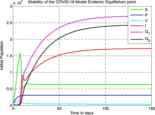
In this subsection, we applied ODE45 programming code and simulated the COVID-19 model given in Equation (2) using parameter values given in Table 3, we have got Figure 2. Figure 2 illustrates that in the near future (after 150 days) the solutions of the transmission dynamics of COVID-19 given in Equation (2) will be converging to its corresponding endemic equilibrium point, i.e. the endemic equilibrium point is locally asymptotically stable if ${\mathcal{R}}_C=10.31>1$. Biologically it means the COVID-19 disease spreads throughout the considered population.

Figure 2. Behaviour of the model solutions whenever ${\mathcal{R}}_C=10.31$ at $\text{β}=\mathrm{0.0013.}$

4.2.2. Effect ${\gamma }_3$ on ${\mathcal{R}}_{\mathit{C}}$

In this section, the numerical simulation given in Figure 3 illustrated that the impact of COVID-19 vaccination rate ${\gamma }_3$ on the COVID-19 effective reproduction number ${\mathcal{R}}_{\text{C}}$. From Figure 3, we have observed that whenever the value of COVID-19 vaccination rate ${\gamma }_3$ increases, the COVID-19 effective reproduction number ${\mathcal{R}}_{\text{C}}$ decreases, and whenever the value of ${\gamma }_3>0.661$ implies ${\mathcal{R}}_C<1.$ Therefore public health policymakers shall concentrate on maximizing the value of COVID-19 vaccination rate ${\gamma }_3$ by more than 0.661 to prevent and control COVID-19 spreading in the community

4.2.3. Effect ${\mathit{\gamma }}_2$ on ${\mathcal{R}}_{\mathit{C}}$

In this section, we have used parameter values given in Table 3 and simulated Figure 4 and from the numerical simulation given in Figure 4, we can determine the impact of COVID-19 protection rate ${\gamma }_2$ on the COVID-19 effective reproduction number ${\mathcal{R}}_{\text{C}}$. Figure 4 illustrated that when the value of COVID-19 protection rate ${\gamma }_2$ increases, the COVID-19 effective reproduction number ${\mathcal{R}}_{\text{C}}$ decreases, and when the value of ${\gamma }_2>0.732$ implies ${\mathcal{R}}_C<1.$ Therefore public health policymakers shall concentrate on maximizing the value of COVID-19 protection rate ${\gamma }_2$ more than 0.732 to prevent and control COVID-19 transmission in the considered population.

4.2.4. Effect ${\mathit{\gamma }}_2$ on ${\mathcal{R}}_{\mathit{C}}$

Here we have simulated the COVID-19 effective reproduction number ${\mathcal{R}}_C$ by applying variable values of COVID-19 transmission rate $\text{β}$ and fixed parameters values in Table 3. Numerical simulation curve given in Figure 5 illustrates that whenever the value of $\text{β}$ increases, the COVID-19 effective reproduction number ${\mathcal{R}}_C$ increases, and if $\text{β}<0.00041$ implies ${\mathcal{R}}_C<1.$ Therefore public health policymakers shall concentrate on decreasing the values of COVID-19 spreading rate $\text{β}$ to minimize COVID-19 effective reproduction number ${\mathcal{R}}_C$. Biologically, it means whenever the COVID-19 transmission rate increases the number of COVID-19 infected individuals increases.

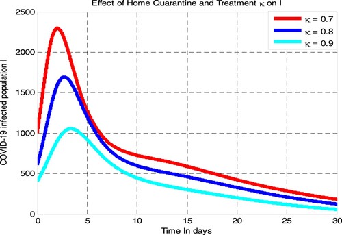
4.2.5. Effect $\mathit{\kappa }$ on COVID-19 infected population

From the numerical simulation curve given in Figure 6, we have determined the effect of COVID-19 home quarantine with treatment rate $\kappa$ on COVID-19 infectious population. Figure 6 shows that if the value of $\kappa$ increases from 0.7 to 0.9 the number of COVID-19 infectious population is going down. Thus, for moderately COVID-19 patients, public health policymakers shall concentrate on increasing the value of COVID-19 home quarantine with treatment rate $\kappa$ to decrease COVID-19 transmission in the community under consideration.

Figure 3. Effect of ${\gamma }_3$ on ${\mathcal{R}}_C$.

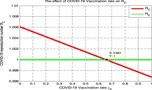
Figure 4. Effect of ${\gamma }_2$ on ${\mathcal{R}}_C.$

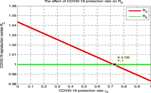
Figure 5. Effect of COVID-19 transmission $\text{β}$ on ${\mathcal{R}}_C.$

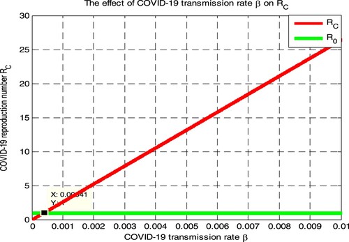
Figure 6. Effect of $\kappa$ on COVID-19 infected population $I.$

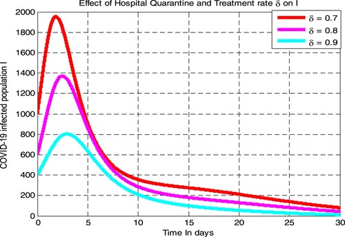
4.2.6. Effect of $\mathit{\delta }$ on COVID-19 infection

From the numerical simulation curve given in Figure 7, we have determined the effect of COVID-19 hospital quarantine with treatment rate $\delta$ on COVID-19 infectious populations. The figure illustrated that if the value of $\delta$ increases from 0.7 to 0.9 the number of COVID-19 infectious population decreases. Therefore for severe COVID-19 infected individuals, public health policymakers shall concentrate on increasing the value of COVID-19 hospital quarantine with treatment rate $\kappa$ to decrease COVID-19 transmission in the considered population.

Figure 7. Effect of $\delta$ on COVID-19 infected population $I.$

5. Discussion

In Section 1, we have introduced the general epidemiology of COVID-19 and reviewed some relevant literature related for this study. In Section 2, we formulated the deterministic compartmental COVID-19 infection dynamical systems using a system of ordinary differential equations and we divided the total human population into six distinct classes. In Section 3, we analysed the model qualitative behaviours such as positivity of future solutions of the COVID-19 infection model, boundedness of the dynamical system, disease-free equilibrium point, effective reproduction number using next-generation approach, endemic equilibrium(s), stability analysis of disease-free equilibrium point, stability analysis of endemic equilibrium point using Routh–Hurwiz criteria, bifurcations analysis of COVID-19 infection model using Center Manifold Theory, sensitivity analysis of effective reproduction number using normalized forward sensitivity index and numerically we experimented on the stability of endemic equilibrium point of the COVID-19 infection model, effect of parameters in the expansion and control of COVID-19 infection, and parameter effect on the effective reproduction number. In Section 4, we have used the MATLAB ODE45 programming code and justified the COVID-19 protection, vaccination, home quarantine with treatment for moderately infected individuals and hospital quarantine with treatment for severely infected individuals’ rates impacts on the COVID-19 infection model in the community. Applying for the intervention measures protection, vaccination, home quarantine with treatment for moderately infected individuals and hospital quarantine with treatment for severely infected individuals’ simultaneously makes the study unique from other scholars' study.

6. Conclusion

In this study, we have formulated and examined a deterministic and compartmental mathematical model for the spreading and controlling of COVID-19 pandemic by incorporating COVID-19 protection, vaccination, home quarantine with treatment for moderately infected individuals, and hospital quarantine with treatment for severely infected individuals in a given community. We have examined the boundedness and positivity of the transmission dynamics model. Using Centre Manifold theory, we have shown that the COVID-19 pandemic undergoes the phenomenon of backward bifurcation if its corresponding effective reproduction number is less than unity. The model has a disease-free equilibrium that is locally-asymptotically stable if its effective reproduction number is less than unity. Numerical simulation shows that the COVID-19 infection model endemic equilibrium point is locally asymptotically stable if its effective reproduction number is greater than unity. The results have important public health implications, as it governs the elimination and/or persistence of the disease in a community. By examining the corresponding effective reproduction number ${\mathcal{R}}_C$, we have determined that the impact of some parameters changes on the corresponding effective reproduction number ${\mathcal{R}}_C$, to give future directions for the stakeholders in the community. From the numerical result, we have got the COVID-19 infection model effective reproduction number ${\mathcal{R}}_C=10.31$ at $\text{β}=0.0013$. From the numerical result, we recommend that public health policymakers shall concentrate on maximizing the values of COVID-19 protection, vaccination, home quarantine with treatment for moderately infected individuals, and hospital quarantine with treatment for severely infected individual’s rates to minimize COVID-19 disease in the community. Finally, some of the main epidemiological findings of this study include COVID-19 protection, vaccination, home quarantine with treatment for moderately infected individuals, and hospital quarantine with treatment for severely infected individuals’ rates to minimize COVID-19 infection expansion and prevalence in the community.

Limitation of the study

Difficulty to incorporate experimental data in the study.

Acknowledgments

The authors would like to thank Mr. Sitotaw Eshete for his Wi-Fi contribution.

Disclosure statement

No potential conflict of interest was reported by the author(s).

Data availability

Data used to support the findings of this study are included in the article.

References

- I. Ahmed, E.F.D. Goufo, A. Yusuf, P. Kumam, P. Chaipanya, and K. Nonlaopon, An epidemic prediction from analysis of a combined HIV-COVID-19 co-infection model via ABC-fractional operator. Alexandria Eng. J. 60(3) (2021), pp. 2979–2995.
- Y.J. Baek, T. Lee, Y. Cho, J.H. Hyun, M.H. Kim, Y. Sohn, J.H. Kim, Sohn Y., Choi J.Y., A mathematical model of COVID-19 transmission in a tertiary hospital and assessment of the effects of different intervention strategies. PloS one 15(10) (2020), pp. e0241169.
- E.A. Bakare, and C.R. Nwozo, Bifurcation and sensitivity analysis of malaria–schistosomiasis co-infection model. Int. J. Appl. Comput. Math. 3(1) (2017), pp. 971–1000.
- C. Castillo-Chavez, and B. Song, Dynamical models of tuberculosis and their applications. Math. Biosci. Eng. 1(2) (2004), pp. 361–404.
- T.-M. Chen, J. Rui, Q.-P. Wang, Z.-Y. Zhao, J.-A. Cui, and L. Yin, A mathematical model for simulating the phase-based transmissibility of a novel coronavirus. Infect. Dis. Poverty. 9(1) (2020), pp. 1–8.
- L. Cirrincione, F. Plescia, C. Ledda, V. Rapisarda, D. Martorana, R.E. Moldovan, K. Theodoridou, and E. Cannizzaro, COVID-19 pandemic: Prevention and protection measures to be adopted at the workplace. Sustainability 12(9) (2020), pp. 3603.
- D.O. Daniel, Mathematical model for the transmission of COVID-19 with nonlinear forces of infection and the need for prevention measure in Nigeria. J. Infect. Dis. Epidem 6 (2021), pp. 158.
- E.E. Endashaw, and T.T. Mekonnen, Modeling the effect of vaccination and treatment on the transmission dynamics of hepatitis B virus and HIV/AIDS coinfection. J. Appl. Math. 2022 (2022), 1–27.
- W. Gao, H.M. Baskonus, and L. Shi, New investigation of bats-hosts-reservoir-people coronavirus model and application to 2019-nCoV system. Adv. Differ. Equ. 2020(1) (2020), pp. 1–11.
- W. Gao, P. Veeresha, H.M. Baskonus, D.G. Prakasha, and P. Kumar, A new study of unreported cases of 2019-nCOV epidemic outbreaks. Chaos, Solitons Fractals 138 (2020), pp. 109929.
- W. Gao, P. Veeresha, D.G. Prakasha, and H.M. Baskonus, Novel dynamic structures of 2019-nCoV with nonlocal operator via powerful computational technique. Biology. (Basel) 9(5) (2020), pp. 107.
- H.A. Gesesew, L. Mwanri, J.H. Stephens, K. Woldemichael, and P. Ward, COVID/HIV co-infection: A syndemic perspective on what to ask and how to answer. Front. Public. Health. 9 (2021), pp. 193.
- A.B. Gumel, J.M.-S. Lubuma, O. Sharomi, and Y.A. Terefe, Mathematics of a sex-structured model for syphilis transmission dynamics. Math. Methods. Appl. Sci. 41(18) (2018), pp. 8488–8513.
- I.M. Hezam, A. Foul, and A. Alrasheedi, A dynamic optimal control model for COVID-19 and cholera co-infection in Yemen. Adv. Differ. Equ. 2021(1) (2021), pp. 1–30.
- A. Kumar, A. Prakash, and H.M. Baskonus, The epidemic COVID-19 model via Caputo–Fabrizio fractional operator. Waves Random Complex Media 32 (2022), pp. 1–15.
- J.Y. Mugisha, J. Ssebuliba, J.N. Nakakawa, C.R. Kikawa, and A. Ssematimba, Mathematical modeling of COVID-19 transmission dynamics in Uganda: Implications of complacency and early easing of lockdown. PloS one 16(2) (2021), pp. e0247456.
- S.S. Musa, I.A. Baba, A. Yusuf, T.A. Sulaiman, A.I. Aliyu, S. Zhao, and D. He, Transmission dynamics of SARS-CoV-2: A modeling analysis with high-and-moderate risk populations. Results Phys. 26 (2021), pp. 104290.
- A. Nwankwo, and D. Okuonghae, Mathematical analysis of the transmission dynamics of HIV syphilis co-infection in the presence of treatment for syphilis. Bull. Math. Biol. 80(3) (2018), pp. 437–492.
- A. Omame, N. Sene, I. Nometa, C.I. Nwakanma, E.U. Nwafor, N.O. Iheonu, and D. Okuonghae, Analysis of COVID-19 and comorbidity co-infection model with optimal control. Optimal Control Appl. Methods 42(6) (2021), pp. 1568–1590.
- P. Riyapan, S.E. Shuaib, and A. Intarasit, A mathematical model of COVID-19 pandemic: A case study of Bangkok, Thailand. Comput. Math. Methods. Med. 2021 (2021), 1–11.
- P. Ssentongo, E.S. Heilbrunn, A.E. Ssentongo, S. Advani, V.M. Chinchilli, J.J. Nunez, and P. Du, Epidemiology and outcomes of COVID-19 in HIV-infected individuals: A systematic review and meta-analysis. Sci. Rep. 11(1) (2021), pp. 1–12.
- D. Sun, X. Long, and J. Liu, Modeling the COVID-19 epidemic with multi-population and control strategies in the United States. Front. Public. Health. 9 (2021), pp. 1–14.
- S.Y. Tchoumi, M.L. Diagne, H. Rwezaura, and J.M. Tchuenche, Malaria and COVID-19 co-dynamics: A mathematical model and optimal control. Appl. Math. Model. 99 (2021), pp. 294–327.
- S.W. Teklu, and B.S. Kotola, The impact of protection measures and treatment on pneumonia infection: A mathematical model analysis supported by numerical simulation. bioRxiv 2022 (2022), pp. 1–22.
- S.W. Teklu, and T.T. Mekonnen, HIV/AIDS-pneumonia co-infection model with treatment at each infection stage: Mathematical analysis and numerical simulation. J. Appl. Math. 2021 (2021), 1–21.
- S.W. Teklu, and K.P. Rao, HIV/AIDS-pneumonia codynamics model analysis with vaccination and treatment. Comput. Math. Methods. Med. 2022 (2022), pp. 1–20.
- S.W. Teklu, and B.B. Terefe, Mathematical modeling analysis on the dynamics of university students’ animosity towards mathematics with optimal control theory. Sci. Rep. 12(1) (2022), pp. 1–19.
- T. Tolossa, R. Tsegaye, S. Shiferaw, B. Wakuma, D. Ayala, B. Bekele, and T. Shibiru, Survival from a triple co-infection of COVID-19, HIV, and tuberculosis: A case report. Int. Med. Case. Rep. J. 14 (2021), pp. 611–615.
- P. Van den Driessche, and J. Watmough, Reproduction numbers and sub-threshold endemic equilibria for compartmental models of disease transmission. Math. Biosci. 180(1-2) (2002), pp. 29–48.
- P. Veeresha, W. Gao, D.G. Prakasha, N.S. Malagi, E. Ilhan, and H.M. Baskonus, New dynamical behaviour of the coronavirus (2019-ncov) infection system with non-local operator from reservoirs to people. Inform. Sci Lett 10(2) (2021), pp. 17.
- I.M. Wangari, S. Sewe, G. Kimathi, M. Wainaina, V. Kitetu, and W. Kaluki, Mathematical modelling of COVID-19 transmission in Kenya: A model with reinfection transmission mechanism. Comput. Math. Methods. Med. 2021 (2021), 1–18.
- H.M. Yang, L.P. Lombardi Junior, F.F.M. Castro, and A.C. Yang, Mathematical modeling of the transmission of SARS-CoV-2, evaluating the impact of isolation in São Paulo State (Brazil) and lockdown in Spain associated with protective measures on the epidemic of CoViD-19. Plos One 16(6) (2021), pp. e0252271.
- A. Zeb, E. Alzahrani, V.S. Erturk, and G. Zaman, Mathematical model for coronavirus disease 2019 (COVID-19) containing isolation class. BioMed Res. Int. 2020 (2020), pp. 1–7.