Deciphering the transmission dynamics of COVID-19 in India: optimal control and cost effective analysis

Abstract

In this paper we assess the effectiveness of different non-pharmaceutical interventions (NPIs) against COVID-19 utilizing a compartmental model. The local asymptotic stability of equilibria (disease-free and endemic) in terms of the basic reproduction number have been determined. We find that the system undergoes a backward bifurcation in the case of imperfect quarantine. The parameters of the model have been estimated from the total confirmed cases of COVID-19 in India. Sensitivity analysis of the basic reproduction number has been performed. The findings also suggest that effectiveness of face masks plays a significant role in reducing the COVID-19 prevalence in India. Optimal control problem with several control strategies has been investigated. We find that the intervention strategies including implementation of lockdown, social distancing, and awareness only, has the highest cost-effectiveness in controlling the infection. This combined strategy also has the least value of average cost-effectiveness ratio (ACER) and associated cost.

Keywords:

• Control strategies
• optimal control
• cost minimization
• COVID-19
• backward bifurcation

Maths:

• 92D30

1. Introduction

At present, the world is confronting the COVID-19 pandemic, caused by a novel coronavirus, SARS-CoV-2, which began as an outbreak of pneumonia of a mysterious cause in Wuhan city of China in December 2019 [45, 70]. Similar to the two previous coronaviruses that triggered significant outbreaks in the human population in recent years (precisely, the Middle Eastern Respiratory Syndrome (MERS) and the Severe Acute Respiratory Syndrome (SARS) [70, 78]), COVID-19 is also spread in humans via direct contact with another infected individual, contaminated surfaces or objects and inhalation of respiratory droplets from both asymptomatic and symptomatic-infectious humans [11]. There are also some evidences that the SARS-CoV-2 virus can be breathe out via regular breathing [52]. In the absence of pharmaceutical interventions (such as an effective and safe vaccine for COVID-19 anti-viral and use in humans), efforts intended for controlling COVID-19 are concentrated on the employment of non-pharmaceutical intervention strategies (NPIs), such as using face-masks, social-distancing, screening, quarantine of suspected cases, hospitalization, and isolation of confirmed cases, mass testing, contact-tracing, etc. Specifically, since the SARS-CoV-2 is transmitted among individuals who got close interactions with each other, using a face mask has been the elementary tool for curtailing the spread of the COVID-19. The use of face-masks in public places has traditionally been an ordinary habit of attempting to combat or bound the transmission of respiratory diseases, dating back to at least the H1N1 1918 influenza pandemic [18, 34, 47, 66]. Face masks may have been involved in regulating the community transmission of the 2002/2003 SARS outbreak in Asia (specifically in Hong Kong, Singapore, China, and Taiwan) [42, 75] as well as the control of the COVID-19 epidemic in Taiwan [69]. Face-masks have two-fold targets. If used by a susceptible person, the mask proposes effectiveness against the acquirement of disease. Additionally, if worn by a diseased individual (but mildly-symptomatic or asymptomatic and unaware that he/she is sick), the face mask shows effectiveness against their capacity to spread the disease to susceptible persons [2, 3, 24, 48, 52].

Numerous mathematical models have been established and utilized to analyse the COVID-19 dynamics with non-pharmaceutical interventions. Ferguson et al. [32] analysed an agent-based model to assess the influences of NPIs on disease-related mortality from COVID-19 and in shrinking the load on health-care equipment and facilities. The authors anticipated that, in the absence of control interventions, over $81\mathrm{\%}$ of Great Britain and the US populations might become infected, and up to 2.2 million deaths may happen by COVID-19 in the US. Ngonghala et al. [53] analysed a mathematical model for COVID-19 and assessed the impact of non-pharmaceutical interventions. Their study shows that using face masks with efficacy greater than $70\mathrm{\%}$ in public, could direct to the eradication of the pandemic if at least $70\mathrm{\%}$ of people wear such masks consistently. Mizumoto et al. [51] modelled a potential outbreak of COVID-19 on the Diamond Princess cruise which faced a major COVID-19 outbreak during January-February, 2020. The authors estimated the reproduction number of the proposed model, which is significantly greater than the estimation reported from the community-level spread in Singapore and China. The study also suggested that the reproduction number significantly decreases with enhancing the effectiveness of the isolation and quarantine measures employed on the ship. Tang et al. [64] proposed a deterministic model based on the clinical development of the disease, intervention measures, and epidemiological characteristics of the people. Their estimations indicate that the control reproduction number may be as high as 6.47. According to sensitivity analysis done in [64], it can be decreased by interventions such as quarantine and isolation.

Due to shortage of resources, optimal employment of intervention strategies should be paramount importance. Optimal control theory presents a way to decide how to utilize one or more time-dependent control interventions to a nonlinear dynamical system in such a regime that a specific objective is optimized [44]. Therefore, in the last few years, countless studies have been established, and numerous control measures are analysed in disease dynamics utilizing optimal control theory [5, 14, 15, 17, 33, 35, 38, 50, 60, 80]. Behncke [15] explored the effect of quarantine, vaccination, health promotional campaigns, and screening as control interventions with the significance of financial support for SIR models. The study discovered that the control interventions reduce the disease level, while financial support encourages promotional campaigns that decrease disease spread during the development of the epidemic. Choi et al. [23] proposed a compartmental model for the tuberculosis (TB) transmission dynamics in South Korea and used the optimal control theory to recommend optimal TB control and prevention interventions and reorganized the government TB budget for the best TB eradication plan. The studies [61, 65] signify that the intensity of NPIs needed is reliant on model parameters. Employment of NPIs may be needed at a high intensity and for a longer time period in the absence of an effective vaccine or drug/medicine. Perkins et al. [55] analysed the optimal control of the COVID-19 pandemic with NPIs via mathematical modelling. The authors considered an optimal strategy in the sense that it includes weighing the relative costs of prevention and disease induced deaths and determined a method to control the pandemic that minimizes the combined cost. Sasmita et al. [60] proposed a deterministic model to analyse the pandemic scenario of COVID-19 in Indonesia and studied the optimal control strategies, namely, large-scale social restriction, use of face masks, contact tracing, mass testing, case detection and treatment. The authors concluded that the scenario including large-scale restriction, case detection and treatment, contact tracing, and use of face masks is the highest effective scenario to regulate the COVID-19 disease in Indonesia. Zamir et al. [81] studied a mathematical model for COVID-19 and explored the optimal control of lockdown, control of disease's side effects, frequent hand wash, using of sanitizer and face mask.

A few authors have also done the cost-effective analysis [1, 7–10, 16, 54]. By performing a cost-effective analysis, it can be recognized that strategies should also to be efficacious and cost-effective. Specifically, forecasting the concerning costs and the respective results of alternate control intervention strategies can be beneficial to policy-makers, who are frequently confronted by the task of resources allocation. Biswas et al. [16] have also examined optimal combinations of control interventions and cost-effective investigation for the transmission of visceral leishmaniasis. Their study suggests that the results would be beneficial for policy/decision-makers to forecast the best control strategies for particular time and their suitable employment for eradicating visceral leishmaniasis. Agusto et al. [1] have analysed the optimal control and cost-effective analysis of malaria/visceral leishmaniasis co-infection. Their results indicate that the strategy merging all the time reliant control variables is the highest cost-effective control intervention strategy. The results were further highlighted expanding the outcomes acquired from the cost objective functional, the ICER, and the ACER. Asamoah et al. [10] proposed and analysed a non-autonomous model to study the control of the COVID-19 in the Kingdom of Saudi Arabia and also investigated the cost-effectiveness analysis for 14 optimal control strategies. The authors concluded that practicing social or physical distancing rules is the most effective and most cost-saving control strategy in Saudi Arabia in the absence of vaccination. Olaniyi et al. [54] studied a mathematical model for COVID-19 considering the transmission paths from asymptotic, symptomatic, and hospitalized persons. The authors also determined the most cost-effective control measure through cost-effectiveness analysis in Nigeria. In order to measure the influence of the environment on the course of COVID-19, Joshua Kiddy et al. [7] presented a compartmental epidemic model adding environment surface. The authors concluded that the optimum method for controlling the disease is a control measure that includes cleaning surfaces with household cleaners. Joshua Kiddy et al. [9] studied a compartmental epidemic model to analyse the optimal control problem and describe the dynamics of COVID-19 for Egypt and Ghana. They discovered that having two controls (transmission reduction and case isolation) is preferable to having only one control, but it is too costly. To better understand the dynamics of Q fever disease transmission, Joshua Kiddy et al. [8] proposed a compartmental epidemic model that included direct transmission cycle, various shedding rates, therapy, and the impact of relapse. The authors designed an optimum control model to investigate the effects of time-dependent treatment, a disinfectant, and separate facilities for animal birthing. Rajput et al. [58] studied a deterministic model with optimal control strategies including vaccination for COVID-19. The authors analysed the model thoroughly and concluded that, to eradicate the COVID-19 disease, it is required to increase the vaccination rate and its efficacy by motivating individuals to take precautionary measures.

The current work is based on developing a novel compartmental model for investigating the transmission dynamics of COVID-19 and control strategies in India. The model acquires the shape of a Kermack–McKendrick, deterministic, compartmental model of nonlinear ordinary differential equations [41]. It includes characteristics related to the transmission dynamics and control of COVID-19, for instance, quarantine of suspected cases, using of face masks, and the hospitalization/isolation of confirmed COVID-19 cases (akin to the models established in [12, 13, 19, 25]). The model is also parameterized utilizing the available cumulative data of COVID-19 in order to estimate the burden of the pandemic in India and assess some of the primary control intervention strategies being employed in the country (particularly, isolation, quarantine, and wearing face-masks in public places). We found that the proposed system undergoes a backward bifurcation when $R_0=1$ in case of low efficacy of quarantine (imperfect quarantine). The backward bifurcation in epidemic models due to imperfect vaccination has been discussed by many researchers [6, 49]. Consequently, the system has two endemic equilibria when $R_0<1$ and $R_0$ below unity is insufficient to eliminate the disease from the population. Therefore, we concluded that in order to control the transmission of COVID-19, the infected individuals need to be kept in quarantine with perfect efficacy. In cost-effectiveness analysis for the optimal control system, we observed that the intervention strategy, including the implementation of lockdown, social distancing, and awareness against COVID-19 infection is the most cost-effective strategy in controlling the disease. This intervention strategy also has the least value of ACER and associated total cost.

The organization of the paper is as follows. In the following section, we formulate the mathematical model for COVID-19. In Section 3, we carry out the rigorous mathematical analysis of the proposed model, including stability and possible bifurcations, final size estimation of COVID-19, threshold dynamics of the basic reproduction number. Numerical simulations and data fitting using the cumulative cases of COVID-19 in India have been presented in Section 4. Optimal control and cost-effective analysis have been discussed in Section 5. The paper ends with a discussion and conclusion in Section 6.

2. Formulation of the mathematical model

We present a nonlinear mathematical model to better explain COVID-19 propagation and control techniques. Our proposed model is based on the Kermac-McKendrick epidemic model and incorporates basic NPIs (including social distancing, contact tracing of diagnosed individuals, random testing and use of face masks in public places and markets, quarantine (home or institutional) of suspected individuals, and isolation (hospitalization or self-isolation) of reported case). The total human population of a community at time t, $N(t)$, is divided into seven compartments based on disease stage, namely non-quarantined susceptible $(Su(t))$, quarantined susceptible $(Sq(t))$, exposed individuals (i.e. newly-infected individuals but cannot transmit COVID-19 to others), $(E(t))$, asymptomatically infectious $(I_a(t))$, symptomatically infectious $(I(t))$, hospitalized/isolated infectious $(I_h(t))$, and recovered $(R(t)).$ Hence, we have $N(t)=S_u(t)+S_q(t)+E(t)+I_a(t)+I(t)+I_h(t)+R(t).$ Those with modest COVID-19 symptoms are included in the asymptomatically infectious compartment $(Ia)$ in this context. According to WHO data, roughly $80\mathrm{\%}$ of COVID-19 reported cases have mild or no symptoms. [71]. A minor type of pneumonia can develop in asymptomatically infectious individuals (particularly, peoples having age $65+$ and older or those with pre-existing health problems), necessitating self-isolation or hospitalization [62, 76, 77, 79]. Furthermore, some individuals in this compartment (particularly those without any clinical symptoms) may be identified (by random sampling or contact tracing of known COVID-19 cases, followed by testing) and placed in self-isolation or institutionalization. Self-isolation or hospitalization for people of the $I_a$ class, or the $I_a$ to $I_h$ transition, is linked to COVID-19 confirmed instances being traced, and then improved testing similar to Iceland [39]. Following the detection of a COVID-19 reported cases (via testing), contact tracing is commenced. Therefore, contact tracing is intimately linked to testing in the proposed model.

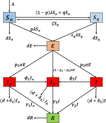
Furthermore, contact tracing can be defined as the procedure of quarantining people reported as having had direct contact with a COVID-19 reported case. Close contact of diagnosed patients, who may have travelled to highly COVID-19 spreading regions or places, (e.g. New York, Italy, China), could also be quarantined in addition to contact tracing. People in quarantine should be susceptible, and their health must always be inspected by the medical expert on a regular basis. People who test positive for COVID-19 are placed in the E class, while those who test negative just after incubation period were transferred to the non-quarantined susceptible class. Therefore, in this problem, we assume that proportion p of those who come into touch with COVID-19-positive people become directly exposed to infection, while the remaining proportion 1−p occurs in quarantine facilities. Isolation and quarantine can take place at home (known as self-quarantine and self-isolation) or in a health care facility (at the authorized centre). In the context of this study, hospitalization encompasses both self-isolation at home and authority-imposed isolation at the hospital. Thus, it would be mentioned that hospitalization and isolation will be used for the same meaning. The flow diagram is presented in Figure 1. The mathematical model which describes the progression of COVID-19 is given by the following deterministic system of nonlinear differential equations: (1) $\begin{array}{rl}\frac{\mathrm{d}{S}_u}{\mathrm{d}t}& =\mathrm{\Lambda }-\lambda S_u-\mathrm{d}{S}_u-q{S}_u+\zeta S_q,\\ \frac{\mathrm{d}{S}_q}{\mathrm{d}t}& =q{S}_u+(1-p)\lambda S_u-({ϵ}_q\lambda +\zeta +d)S_q,\\ \frac{\mathrm{d}E}{\mathrm{d}t}& =p\lambda S_u+{ϵ}_q\lambda S_q-(\alpha +d)E,\\ \frac{\mathrm{d}{I}_a}{\mathrm{d}t}& =p_1\alpha E-({\delta }_1+{\varphi }_1+{\gamma }_1+d)I_a,\\ \frac{\mathrm{d}I}{\mathrm{d}t}& =p_2\alpha E-({\delta }_2+{\varphi }_2+{\gamma }_2+d)I,\\ \frac{\mathrm{d}{I}_h}{\mathrm{d}t}& =(1-p_1-p_2)\alpha E+{\varphi }_1{I}_a+{\varphi }_{2}I-({\delta }_3+{\gamma }_3+d)I_h,\\ \frac{\mathrm{d}R}{\mathrm{d}t}& ={\gamma }_1{I}_a+{\gamma }_{2}I+{\gamma }_3{I}_h-\mathrm{d}R,\end{array}$(1) where $\lambda =\frac{\beta (1-p_M{ϵ}_M)(I+{\psi }_a{I}_a+{\psi }_h{I}_h)}{N-{ϵ}_h{I}_h}.$ In the proposed model (1(1) $\begin{array}{rl}\frac{\mathrm{d}{S}_u}{\mathrm{d}t}& =\mathrm{\Lambda }-\lambda S_u-\mathrm{d}{S}_u-q{S}_u+\zeta S_q,\\ \frac{\mathrm{d}{S}_q}{\mathrm{d}t}& =q{S}_u+(1-p)\lambda S_u-({ϵ}_q\lambda +\zeta +d)S_q,\\ \frac{\mathrm{d}E}{\mathrm{d}t}& =p\lambda S_u+{ϵ}_q\lambda S_q-(\alpha +d)E,\\ \frac{\mathrm{d}{I}_a}{\mathrm{d}t}& =p_1\alpha E-({\delta }_1+{\varphi }_1+{\gamma }_1+d)I_a,\\ \frac{\mathrm{d}I}{\mathrm{d}t}& =p_2\alpha E-({\delta }_2+{\varphi }_2+{\gamma }_2+d)I,\\ \frac{\mathrm{d}{I}_h}{\mathrm{d}t}& =(1-p_1-p_2)\alpha E+{\varphi }_1{I}_a+{\varphi }_{2}I-({\delta }_3+{\gamma }_3+d)I_h,\\ \frac{\mathrm{d}R}{\mathrm{d}t}& ={\gamma }_1{I}_a+{\gamma }_{2}I+{\gamma }_3{I}_h-\mathrm{d}R,\end{array}$(1) ), β is the adequate contact rate in terms of the number of contacts per unit time between susceptible and an infectious individual, which is capable of COVID-19 transmission. The reduction factor $(1-p_M{ϵ}_M)$ in the parameter β can be interpreted as a measure of the performance of control techniques that reduce human interaction in order to prevent the spread of COVID-19 in the community, particularly the wearing of face masks. $0<p_M\le 1$ is the proportion of individuals in the community who use the face-masks in public places. The physical interpretation of $0<p_M\le 1$ is that small value of $p_M$ imply very limited individuals are using the face-masks, while value of $p_M$ is near to one imply face masks are widely/universally used in the community. The parameter $0<{ϵ}_M\le 1$ measures the efficiency of face-masks in sense that ${ϵ}_M$ significantly closed to zero implies that the face-masks are very little effective to avoid infection, while ${ϵ}_M$ close, or equal to, unity implies that face masks are getting closer to complete efficacy against illness acquisition and transmission. $0<{\psi }_a<1$ represents the relative infectiousness of the $I_a$ class compared to that of the I class. Similarly, $0<{\psi }_h<1$ quantifies the relative infectiousness of isolated infectious individuals concerning individuals in the I class. The parameter $0<{ϵ}_h\le 1$ measures the effectiveness of isolation to prevent isolated infectious individuals from spreading COVID-19 infection. Precisely, ${ϵ}_h=1$ implies that isolated infectious individuals are no longer part of the actively-mixing population and do not contribute to COVID-19 transmission. The modification parameter $0\le {ϵ}_q\le 1$ assesses the effectiveness of quarantine in preventing infection among quarantined-susceptible people during the quarantine period. Biological interpretations of the model parameters are also given in Table 1. The initial conditions of model (1(1) $\begin{array}{rl}\frac{\mathrm{d}{S}_u}{\mathrm{d}t}& =\mathrm{\Lambda }-\lambda S_u-\mathrm{d}{S}_u-q{S}_u+\zeta S_q,\\ \frac{\mathrm{d}{S}_q}{\mathrm{d}t}& =q{S}_u+(1-p)\lambda S_u-({ϵ}_q\lambda +\zeta +d)S_q,\\ \frac{\mathrm{d}E}{\mathrm{d}t}& =p\lambda S_u+{ϵ}_q\lambda S_q-(\alpha +d)E,\\ \frac{\mathrm{d}{I}_a}{\mathrm{d}t}& =p_1\alpha E-({\delta }_1+{\varphi }_1+{\gamma }_1+d)I_a,\\ \frac{\mathrm{d}I}{\mathrm{d}t}& =p_2\alpha E-({\delta }_2+{\varphi }_2+{\gamma }_2+d)I,\\ \frac{\mathrm{d}{I}_h}{\mathrm{d}t}& =(1-p_1-p_2)\alpha E+{\varphi }_1{I}_a+{\varphi }_{2}I-({\delta }_3+{\gamma }_3+d)I_h,\\ \frac{\mathrm{d}R}{\mathrm{d}t}& ={\gamma }_1{I}_a+{\gamma }_{2}I+{\gamma }_3{I}_h-\mathrm{d}R,\end{array}$(1) ) are considered as (2) $S_u(0)>0,S_q(0)\ge 0,E(0)\ge 0,I_a(0)\ge 0,I(0)\ge 0,I_h(0)\ge 0,R(0)\ge 0.$(2)

Figure 1. Flow diagram of model (1(1) $\begin{array}{rl}\frac{\mathrm{d}{S}_u}{\mathrm{d}t}& =\mathrm{\Lambda }-\lambda S_u-\mathrm{d}{S}_u-q{S}_u+\zeta S_q,\\ \frac{\mathrm{d}{S}_q}{\mathrm{d}t}& =q{S}_u+(1-p)\lambda S_u-({ϵ}_q\lambda +\zeta +d)S_q,\\ \frac{\mathrm{d}E}{\mathrm{d}t}& =p\lambda S_u+{ϵ}_q\lambda S_q-(\alpha +d)E,\\ \frac{\mathrm{d}{I}_a}{\mathrm{d}t}& =p_1\alpha E-({\delta }_1+{\varphi }_1+{\gamma }_1+d)I_a,\\ \frac{\mathrm{d}I}{\mathrm{d}t}& =p_2\alpha E-({\delta }_2+{\varphi }_2+{\gamma }_2+d)I,\\ \frac{\mathrm{d}{I}_h}{\mathrm{d}t}& =(1-p_1-p_2)\alpha E+{\varphi }_1{I}_a+{\varphi }_{2}I-({\delta }_3+{\gamma }_3+d)I_h,\\ \frac{\mathrm{d}R}{\mathrm{d}t}& ={\gamma }_1{I}_a+{\gamma }_{2}I+{\gamma }_3{I}_h-\mathrm{d}R,\end{array}$(1) ).

3. Mathematical analysis

3.1. Well-posedness

We first prove the non-negativity and boundedness of the solutions of model system (1(1) $\begin{array}{rl}\frac{\mathrm{d}{S}_u}{\mathrm{d}t}& =\mathrm{\Lambda }-\lambda S_u-\mathrm{d}{S}_u-q{S}_u+\zeta S_q,\\ \frac{\mathrm{d}{S}_q}{\mathrm{d}t}& =q{S}_u+(1-p)\lambda S_u-({ϵ}_q\lambda +\zeta +d)S_q,\\ \frac{\mathrm{d}E}{\mathrm{d}t}& =p\lambda S_u+{ϵ}_q\lambda S_q-(\alpha +d)E,\\ \frac{\mathrm{d}{I}_a}{\mathrm{d}t}& =p_1\alpha E-({\delta }_1+{\varphi }_1+{\gamma }_1+d)I_a,\\ \frac{\mathrm{d}I}{\mathrm{d}t}& =p_2\alpha E-({\delta }_2+{\varphi }_2+{\gamma }_2+d)I,\\ \frac{\mathrm{d}{I}_h}{\mathrm{d}t}& =(1-p_1-p_2)\alpha E+{\varphi }_1{I}_a+{\varphi }_{2}I-({\delta }_3+{\gamma }_3+d)I_h,\\ \frac{\mathrm{d}R}{\mathrm{d}t}& ={\gamma }_1{I}_a+{\gamma }_{2}I+{\gamma }_3{I}_h-\mathrm{d}R,\end{array}$(1) ) to show the the biological feasibility of it. We show that all the solutions of the system (1(1) $\begin{array}{rl}\frac{\mathrm{d}{S}_u}{\mathrm{d}t}& =\mathrm{\Lambda }-\lambda S_u-\mathrm{d}{S}_u-q{S}_u+\zeta S_q,\\ \frac{\mathrm{d}{S}_q}{\mathrm{d}t}& =q{S}_u+(1-p)\lambda S_u-({ϵ}_q\lambda +\zeta +d)S_q,\\ \frac{\mathrm{d}E}{\mathrm{d}t}& =p\lambda S_u+{ϵ}_q\lambda S_q-(\alpha +d)E,\\ \frac{\mathrm{d}{I}_a}{\mathrm{d}t}& =p_1\alpha E-({\delta }_1+{\varphi }_1+{\gamma }_1+d)I_a,\\ \frac{\mathrm{d}I}{\mathrm{d}t}& =p_2\alpha E-({\delta }_2+{\varphi }_2+{\gamma }_2+d)I,\\ \frac{\mathrm{d}{I}_h}{\mathrm{d}t}& =(1-p_1-p_2)\alpha E+{\varphi }_1{I}_a+{\varphi }_{2}I-({\delta }_3+{\gamma }_3+d)I_h,\\ \frac{\mathrm{d}R}{\mathrm{d}t}& ={\gamma }_1{I}_a+{\gamma }_{2}I+{\gamma }_3{I}_h-\mathrm{d}R,\end{array}$(1) ) are non-negative with non-negative initial values of it (2(2) $S_u(0)>0,S_q(0)\ge 0,E(0)\ge 0,I_a(0)\ge 0,I(0)\ge 0,I_h(0)\ge 0,R(0)\ge 0.$(2) ), i.e.$S_u(t)>0,S_q(t)\ge 0,E(t)\ge 0,I_a(t)\ge 0,I(t)\ge 0,I_h(t)\ge 0,R(t)\ge 0$ for all $t\ge 0.$ First, we will prove that $S_u(t)>0$ for all time $t\ge 0.$ For this, we suppose that there exists a time $t_1>0$ such that $S_u(t_1)=0$ and $S_u(t)>0$ for $0<t<t_1.$ Therefore, by the first equation of system (1(1) $\begin{array}{rl}\frac{\mathrm{d}{S}_u}{\mathrm{d}t}& =\mathrm{\Lambda }-\lambda S_u-\mathrm{d}{S}_u-q{S}_u+\zeta S_q,\\ \frac{\mathrm{d}{S}_q}{\mathrm{d}t}& =q{S}_u+(1-p)\lambda S_u-({ϵ}_q\lambda +\zeta +d)S_q,\\ \frac{\mathrm{d}E}{\mathrm{d}t}& =p\lambda S_u+{ϵ}_q\lambda S_q-(\alpha +d)E,\\ \frac{\mathrm{d}{I}_a}{\mathrm{d}t}& =p_1\alpha E-({\delta }_1+{\varphi }_1+{\gamma }_1+d)I_a,\\ \frac{\mathrm{d}I}{\mathrm{d}t}& =p_2\alpha E-({\delta }_2+{\varphi }_2+{\gamma }_2+d)I,\\ \frac{\mathrm{d}{I}_h}{\mathrm{d}t}& =(1-p_1-p_2)\alpha E+{\varphi }_1{I}_a+{\varphi }_{2}I-({\delta }_3+{\gamma }_3+d)I_h,\\ \frac{\mathrm{d}R}{\mathrm{d}t}& ={\gamma }_1{I}_a+{\gamma }_{2}I+{\gamma }_3{I}_h-\mathrm{d}R,\end{array}$(1) ), we obtain $\frac{\mathrm{d}{S}_u(t_1)}{\mathrm{d}t}=\mathrm{\Lambda }+\zeta S_q>0,$ Since $\frac{\mathrm{d}{S}_u}{\mathrm{d}t}>0$ when $S_u$ is small, there is a contradiction to $S_u(t_1)=0.$ Hence, $S_u$ remains positive for all t>0 with $S_u(0)>0.$ Next, from the second equation of model (1(1) $\begin{array}{rl}\frac{\mathrm{d}{S}_u}{\mathrm{d}t}& =\mathrm{\Lambda }-\lambda S_u-\mathrm{d}{S}_u-q{S}_u+\zeta S_q,\\ \frac{\mathrm{d}{S}_q}{\mathrm{d}t}& =q{S}_u+(1-p)\lambda S_u-({ϵ}_q\lambda +\zeta +d)S_q,\\ \frac{\mathrm{d}E}{\mathrm{d}t}& =p\lambda S_u+{ϵ}_q\lambda S_q-(\alpha +d)E,\\ \frac{\mathrm{d}{I}_a}{\mathrm{d}t}& =p_1\alpha E-({\delta }_1+{\varphi }_1+{\gamma }_1+d)I_a,\\ \frac{\mathrm{d}I}{\mathrm{d}t}& =p_2\alpha E-({\delta }_2+{\varphi }_2+{\gamma }_2+d)I,\\ \frac{\mathrm{d}{I}_h}{\mathrm{d}t}& =(1-p_1-p_2)\alpha E+{\varphi }_1{I}_a+{\varphi }_{2}I-({\delta }_3+{\gamma }_3+d)I_h,\\ \frac{\mathrm{d}R}{\mathrm{d}t}& ={\gamma }_1{I}_a+{\gamma }_{2}I+{\gamma }_3{I}_h-\mathrm{d}R,\end{array}$(1) ), we obtain $S_q(t)\ge S_q(0)\exp (-({ϵ}_q\lambda +\zeta +d)t)\ge 0.$ Therefore, we have $S_q(t)\ge 0$ for $t\ge 0.$ The non-negativity of other variables can be proved in a similar fashion.

Table 1. Biological interpretation of the model parameters used in system (1(1) $\begin{array}{rl}\frac{\mathrm{d}{S}_u}{\mathrm{d}t}& =\mathrm{\Lambda }-\lambda S_u-\mathrm{d}{S}_u-q{S}_u+\zeta S_q,\\ \frac{\mathrm{d}{S}_q}{\mathrm{d}t}& =q{S}_u+(1-p)\lambda S_u-({ϵ}_q\lambda +\zeta +d)S_q,\\ \frac{\mathrm{d}E}{\mathrm{d}t}& =p\lambda S_u+{ϵ}_q\lambda S_q-(\alpha +d)E,\\ \frac{\mathrm{d}{I}_a}{\mathrm{d}t}& =p_1\alpha E-({\delta }_1+{\varphi }_1+{\gamma }_1+d)I_a,\\ \frac{\mathrm{d}I}{\mathrm{d}t}& =p_2\alpha E-({\delta }_2+{\varphi }_2+{\gamma }_2+d)I,\\ \frac{\mathrm{d}{I}_h}{\mathrm{d}t}& =(1-p_1-p_2)\alpha E+{\varphi }_1{I}_a+{\varphi }_{2}I-({\delta }_3+{\gamma }_3+d)I_h,\\ \frac{\mathrm{d}R}{\mathrm{d}t}& ={\gamma }_1{I}_a+{\gamma }_{2}I+{\gamma }_3{I}_h-\mathrm{d}R,\end{array}$(1) ).

Parameter	Biological interpretation
Λ	Requirement rate
β	Transmission coefficient in the absence of control measures
$p_M$	Proportion of individuals who use face-masks in public
${ϵ}_M$	Measure the effectiveness of face- masks in avoiding COVID-19 infection
p	Proportion of individuals who become exposed after a contact with an infectious individual.
d	The natural death rate of individuals
ζ	Rate at which the quarantined individuals go back to susceptible class $(S_u)$
${ϵ}_q$	Measures the efficacy of quarantine to avert COVID-19 transmission during quarantine
${\psi }_a({\psi }_h)$	Modification factor for the infectiousness of asymptomatically (isolated) infectious individuals
${ϵ}_h$	Measures the effectiveness of isolation in preventing the transmission of COVID-19 disease in a hospital or isolation site.
$\frac{1}{\alpha }$	Incubation period for exposed individuals
$p_1(p_2)$	Proportion of exposed individuals who enter to the $I_a(I)$ classes after the incubation period
$1-(p_1+p_2)$	Proportion of exposed individuals who move to the $I_h$ class at the end the incubation period (after diagnosed)
${\delta }_1({\delta }_2)({\delta }_3)$	COVID-19 infection induced death rate of individuals in the $I_a(I)(I_h)$ classes
${\gamma }_1({\gamma }_2)({\gamma }_3)$	Recovery rate for the $I_a(I)(I_h)$ classes
${\varphi }_1({\varphi }_2)$	Isolation/hospitalization rate for individuals in the $I_a(I)$ classes after diagnosis

To demonstrate the boundedness of the model system (1(1) $\begin{array}{rl}\frac{\mathrm{d}{S}_u}{\mathrm{d}t}& =\mathrm{\Lambda }-\lambda S_u-\mathrm{d}{S}_u-q{S}_u+\zeta S_q,\\ \frac{\mathrm{d}{S}_q}{\mathrm{d}t}& =q{S}_u+(1-p)\lambda S_u-({ϵ}_q\lambda +\zeta +d)S_q,\\ \frac{\mathrm{d}E}{\mathrm{d}t}& =p\lambda S_u+{ϵ}_q\lambda S_q-(\alpha +d)E,\\ \frac{\mathrm{d}{I}_a}{\mathrm{d}t}& =p_1\alpha E-({\delta }_1+{\varphi }_1+{\gamma }_1+d)I_a,\\ \frac{\mathrm{d}I}{\mathrm{d}t}& =p_2\alpha E-({\delta }_2+{\varphi }_2+{\gamma }_2+d)I,\\ \frac{\mathrm{d}{I}_h}{\mathrm{d}t}& =(1-p_1-p_2)\alpha E+{\varphi }_1{I}_a+{\varphi }_{2}I-({\delta }_3+{\gamma }_3+d)I_h,\\ \frac{\mathrm{d}R}{\mathrm{d}t}& ={\gamma }_1{I}_a+{\gamma }_{2}I+{\gamma }_3{I}_h-\mathrm{d}R,\end{array}$(1) ), solutions, we add all equations of system (1(1) $\begin{array}{rl}\frac{\mathrm{d}{S}_u}{\mathrm{d}t}& =\mathrm{\Lambda }-\lambda S_u-\mathrm{d}{S}_u-q{S}_u+\zeta S_q,\\ \frac{\mathrm{d}{S}_q}{\mathrm{d}t}& =q{S}_u+(1-p)\lambda S_u-({ϵ}_q\lambda +\zeta +d)S_q,\\ \frac{\mathrm{d}E}{\mathrm{d}t}& =p\lambda S_u+{ϵ}_q\lambda S_q-(\alpha +d)E,\\ \frac{\mathrm{d}{I}_a}{\mathrm{d}t}& =p_1\alpha E-({\delta }_1+{\varphi }_1+{\gamma }_1+d)I_a,\\ \frac{\mathrm{d}I}{\mathrm{d}t}& =p_2\alpha E-({\delta }_2+{\varphi }_2+{\gamma }_2+d)I,\\ \frac{\mathrm{d}{I}_h}{\mathrm{d}t}& =(1-p_1-p_2)\alpha E+{\varphi }_1{I}_a+{\varphi }_{2}I-({\delta }_3+{\gamma }_3+d)I_h,\\ \frac{\mathrm{d}R}{\mathrm{d}t}& ={\gamma }_1{I}_a+{\gamma }_{2}I+{\gamma }_3{I}_h-\mathrm{d}R,\end{array}$(1) ), which yields: $\frac{\mathrm{d}N}{\mathrm{d}t}=\mathrm{\Lambda }-\mathrm{d}N-{\delta }_1{I}_a-{\delta }_{2}I-{\delta }_3{I}_h⟹\mathrm{\Lambda }-(d+{\delta }_1+{\delta }_2+{\delta }_3)N\le \frac{\mathrm{d}N}{\mathrm{d}t}\le \mathrm{\Lambda }-\mathrm{d}N.$ The above inequality implies that $\frac{\mathrm{d}N}{\mathrm{d}t}$ is bounded above as well below. Now by integrating and using the initial total population, we can easily obtain $\begin{array}{rl}& \frac{\mathrm{\Lambda }}{(d+{\delta }_1+{\delta }_2+{\delta }_3)}+(N(0)-\frac{\mathrm{\Lambda }}{(d+{\delta }_1+{\delta }_2+{\delta }_3)})e^{-(d+{\delta }_1+{\delta }_2+{\delta }_3)t}\\ & \le N(t)\le \frac{\mathrm{\Lambda }}{d}+(N(0)-\frac{\mathrm{\Lambda }}{d})e^{-\mathrm{d}t}.\end{array}$ Considering $t\to \mathrm{\infty },$ we obtain $\begin{array}{rl}& \frac{\mathrm{\Lambda }}{(d+{\delta }_1+{\delta }_2+{\delta }_3)}\\ & \le \underset{t\to \mathrm{\infty }}{lim inf}N(t)\le \underset{t\to \mathrm{\infty }}{lim sup}N(t)\le \frac{\mathrm{\Lambda }}{d}⟹\frac{\mathrm{\Lambda }}{(d+{\delta }_1+{\delta }_2+{\delta }_3)}\le N(t)\le \frac{\mathrm{\Lambda }}{d}.\end{array}$ Hence the feasible region for the model system (1(1) $\begin{array}{rl}\frac{\mathrm{d}{S}_u}{\mathrm{d}t}& =\mathrm{\Lambda }-\lambda S_u-\mathrm{d}{S}_u-q{S}_u+\zeta S_q,\\ \frac{\mathrm{d}{S}_q}{\mathrm{d}t}& =q{S}_u+(1-p)\lambda S_u-({ϵ}_q\lambda +\zeta +d)S_q,\\ \frac{\mathrm{d}E}{\mathrm{d}t}& =p\lambda S_u+{ϵ}_q\lambda S_q-(\alpha +d)E,\\ \frac{\mathrm{d}{I}_a}{\mathrm{d}t}& =p_1\alpha E-({\delta }_1+{\varphi }_1+{\gamma }_1+d)I_a,\\ \frac{\mathrm{d}I}{\mathrm{d}t}& =p_2\alpha E-({\delta }_2+{\varphi }_2+{\gamma }_2+d)I,\\ \frac{\mathrm{d}{I}_h}{\mathrm{d}t}& =(1-p_1-p_2)\alpha E+{\varphi }_1{I}_a+{\varphi }_{2}I-({\delta }_3+{\gamma }_3+d)I_h,\\ \frac{\mathrm{d}R}{\mathrm{d}t}& ={\gamma }_1{I}_a+{\gamma }_{2}I+{\gamma }_3{I}_h-\mathrm{d}R,\end{array}$(1) ) is (3) $\begin{array}{rl}\mathrm{\Omega }& =\{\phantom{\frac{\mathrm{\Lambda }}{(d+{\delta }_1+{\delta }_2+{\delta }_3)}}(S_u,S_q,E,I_a,I,I_h,R)\in {\mathbb{R}}_{+}^7:\\ & \frac{\mathrm{\Lambda }}{(d+{\delta }_1+{\delta }_2+{\delta }_3)}\le S_u+S_q+E+I_a+I+I_h+R\le \frac{\mathrm{\Lambda }}{d}\subset {\mathbb{R}}_{+}^7\}.\end{array}$(3) Hence, Ω is the bounded region for the solutions of the system (1(1) $\begin{array}{rl}\frac{\mathrm{d}{S}_u}{\mathrm{d}t}& =\mathrm{\Lambda }-\lambda S_u-\mathrm{d}{S}_u-q{S}_u+\zeta S_q,\\ \frac{\mathrm{d}{S}_q}{\mathrm{d}t}& =q{S}_u+(1-p)\lambda S_u-({ϵ}_q\lambda +\zeta +d)S_q,\\ \frac{\mathrm{d}E}{\mathrm{d}t}& =p\lambda S_u+{ϵ}_q\lambda S_q-(\alpha +d)E,\\ \frac{\mathrm{d}{I}_a}{\mathrm{d}t}& =p_1\alpha E-({\delta }_1+{\varphi }_1+{\gamma }_1+d)I_a,\\ \frac{\mathrm{d}I}{\mathrm{d}t}& =p_2\alpha E-({\delta }_2+{\varphi }_2+{\gamma }_2+d)I,\\ \frac{\mathrm{d}{I}_h}{\mathrm{d}t}& =(1-p_1-p_2)\alpha E+{\varphi }_1{I}_a+{\varphi }_{2}I-({\delta }_3+{\gamma }_3+d)I_h,\\ \frac{\mathrm{d}R}{\mathrm{d}t}& ={\gamma }_1{I}_a+{\gamma }_{2}I+{\gamma }_3{I}_h-\mathrm{d}R,\end{array}$(1) ). From the above analysis, the non-negativity and boundedness summarize in the following result:

Theorem 3.1

The solutions of the system (1(1) $\begin{array}{rl}\frac{\mathrm{d}{S}_u}{\mathrm{d}t}& =\mathrm{\Lambda }-\lambda S_u-\mathrm{d}{S}_u-q{S}_u+\zeta S_q,\\ \frac{\mathrm{d}{S}_q}{\mathrm{d}t}& =q{S}_u+(1-p)\lambda S_u-({ϵ}_q\lambda +\zeta +d)S_q,\\ \frac{\mathrm{d}E}{\mathrm{d}t}& =p\lambda S_u+{ϵ}_q\lambda S_q-(\alpha +d)E,\\ \frac{\mathrm{d}{I}_a}{\mathrm{d}t}& =p_1\alpha E-({\delta }_1+{\varphi }_1+{\gamma }_1+d)I_a,\\ \frac{\mathrm{d}I}{\mathrm{d}t}& =p_2\alpha E-({\delta }_2+{\varphi }_2+{\gamma }_2+d)I,\\ \frac{\mathrm{d}{I}_h}{\mathrm{d}t}& =(1-p_1-p_2)\alpha E+{\varphi }_1{I}_a+{\varphi }_{2}I-({\delta }_3+{\gamma }_3+d)I_h,\\ \frac{\mathrm{d}R}{\mathrm{d}t}& ={\gamma }_1{I}_a+{\gamma }_{2}I+{\gamma }_3{I}_h-\mathrm{d}R,\end{array}$(1) ) with initial conditions (2(2) $S_u(0)>0,S_q(0)\ge 0,E(0)\ge 0,I_a(0)\ge 0,I(0)\ge 0,I_h(0)\ge 0,R(0)\ge 0.$(2) ) remain non-negative with the advancement of time. Moreover, the closed region Ω is positively invariant under the flow of model system (1(1) $\begin{array}{rl}\frac{\mathrm{d}{S}_u}{\mathrm{d}t}& =\mathrm{\Lambda }-\lambda S_u-\mathrm{d}{S}_u-q{S}_u+\zeta S_q,\\ \frac{\mathrm{d}{S}_q}{\mathrm{d}t}& =q{S}_u+(1-p)\lambda S_u-({ϵ}_q\lambda +\zeta +d)S_q,\\ \frac{\mathrm{d}E}{\mathrm{d}t}& =p\lambda S_u+{ϵ}_q\lambda S_q-(\alpha +d)E,\\ \frac{\mathrm{d}{I}_a}{\mathrm{d}t}& =p_1\alpha E-({\delta }_1+{\varphi }_1+{\gamma }_1+d)I_a,\\ \frac{\mathrm{d}I}{\mathrm{d}t}& =p_2\alpha E-({\delta }_2+{\varphi }_2+{\gamma }_2+d)I,\\ \frac{\mathrm{d}{I}_h}{\mathrm{d}t}& =(1-p_1-p_2)\alpha E+{\varphi }_1{I}_a+{\varphi }_{2}I-({\delta }_3+{\gamma }_3+d)I_h,\\ \frac{\mathrm{d}R}{\mathrm{d}t}& ={\gamma }_1{I}_a+{\gamma }_{2}I+{\gamma }_3{I}_h-\mathrm{d}R,\end{array}$(1) ).

3.2. Disease-free equilibrium and basic reproduction number

The model system (1(1) $\begin{array}{rl}\frac{\mathrm{d}{S}_u}{\mathrm{d}t}& =\mathrm{\Lambda }-\lambda S_u-\mathrm{d}{S}_u-q{S}_u+\zeta S_q,\\ \frac{\mathrm{d}{S}_q}{\mathrm{d}t}& =q{S}_u+(1-p)\lambda S_u-({ϵ}_q\lambda +\zeta +d)S_q,\\ \frac{\mathrm{d}E}{\mathrm{d}t}& =p\lambda S_u+{ϵ}_q\lambda S_q-(\alpha +d)E,\\ \frac{\mathrm{d}{I}_a}{\mathrm{d}t}& =p_1\alpha E-({\delta }_1+{\varphi }_1+{\gamma }_1+d)I_a,\\ \frac{\mathrm{d}I}{\mathrm{d}t}& =p_2\alpha E-({\delta }_2+{\varphi }_2+{\gamma }_2+d)I,\\ \frac{\mathrm{d}{I}_h}{\mathrm{d}t}& =(1-p_1-p_2)\alpha E+{\varphi }_1{I}_a+{\varphi }_{2}I-({\delta }_3+{\gamma }_3+d)I_h,\\ \frac{\mathrm{d}R}{\mathrm{d}t}& ={\gamma }_1{I}_a+{\gamma }_{2}I+{\gamma }_3{I}_h-\mathrm{d}R,\end{array}$(1) ) has a disease free equilibrium (DFE) $P^0=(S_a^0,S_q^0,E^0,I_a^0,I^0,I_h^0,R^0)=(\frac{(d+\zeta )\mathrm{\Lambda }}{d(d+q+\zeta )},\frac{q\mathrm{\Lambda }}{d(d+q+\zeta )},0,0,0,0,0).$ In addition, the basic reproduction number $(R_0)$ is determined, which serves as a key threshold in the epidemic model. $R_0$ is the average number of secondary infections caused by an infectious person in a community of susceptible individuals during its infectious phase. If the value of $R_0$ is less than 1, an infected person cannot cause an outbreak. If $R_0$ is greater than 1, the number of secondary cases increases, resulting in an outbreak until the fraction of susceptible individuals falls. The next generation matrix approach [67] is used to calculate the basic reproduction number. For this, we rewrite the equations associated to infectious compartments of system (1(1) $\begin{array}{rl}\frac{\mathrm{d}{S}_u}{\mathrm{d}t}& =\mathrm{\Lambda }-\lambda S_u-\mathrm{d}{S}_u-q{S}_u+\zeta S_q,\\ \frac{\mathrm{d}{S}_q}{\mathrm{d}t}& =q{S}_u+(1-p)\lambda S_u-({ϵ}_q\lambda +\zeta +d)S_q,\\ \frac{\mathrm{d}E}{\mathrm{d}t}& =p\lambda S_u+{ϵ}_q\lambda S_q-(\alpha +d)E,\\ \frac{\mathrm{d}{I}_a}{\mathrm{d}t}& =p_1\alpha E-({\delta }_1+{\varphi }_1+{\gamma }_1+d)I_a,\\ \frac{\mathrm{d}I}{\mathrm{d}t}& =p_2\alpha E-({\delta }_2+{\varphi }_2+{\gamma }_2+d)I,\\ \frac{\mathrm{d}{I}_h}{\mathrm{d}t}& =(1-p_1-p_2)\alpha E+{\varphi }_1{I}_a+{\varphi }_{2}I-({\delta }_3+{\gamma }_3+d)I_h,\\ \frac{\mathrm{d}R}{\mathrm{d}t}& ={\gamma }_1{I}_a+{\gamma }_{2}I+{\gamma }_3{I}_h-\mathrm{d}R,\end{array}$(1) ) as follows: $x^{\mathrm{\prime }}=\mathcal{F}-\mathcal{V}$, where $x=(E,I_a,I,I_h{)}^T\in {\mathbb{R}}^4,$ $\mathcal{F}=\left(\begin{array}{c}p\lambda S_u+{ϵ}_q\lambda S_q\\ 0\\ 0\\ 0\end{array}\right),\mathrm{and}\mathcal{V}=\left(\begin{array}{c}(d+\alpha )E\\ K_1{I}_a-p_1\alpha E\\ K_{2}I-p_2\alpha E\\ I_h{K}_3-{\varphi }_{2}I-{\varphi }_1{I}_a-E(1-p_1-p_2)\alpha \end{array}\right).$ Further, we calculate the Jacobian F and V at the $P^0,$ which is given as $\begin{array}{rl}F& ={\frac{\mathrm{d}{\mathcal{F}}_i}{\mathrm{d}{x}_j}}_{|E^0}\\ & =(\begin{array}{cc}0& {\displaystyle \frac{\beta (1-p_M{ϵ}_M)(\mathrm{d}p+q{ϵ}_q+p\zeta ){\psi }_a}{d+q+\zeta }}\\ 0& 0\\ 0& 0\\ 0& 0\end{array}\\ & \begin{array}{cc}{\displaystyle \frac{\beta (1-p_M{ϵ}_M)(\mathrm{d}p+q{ϵ}_q+p\zeta )}{d+q+\zeta }}& {\displaystyle \frac{\beta (1-p_M{ϵ}_M)(\mathrm{d}p+q{ϵ}_q+p\zeta ){\psi }_h}{d+q+\zeta }}\\ 0& 0\\ 0& 0\\ 0& 0\end{array}),\\ \mathrm{\Sigma }& ={\frac{\mathrm{d}{\mathcal{V}}_i}{d{x}_j}}_{|E^0}=\left(\begin{array}{cccc}d+\alpha & 0& 0& 0\\ -p_1\alpha & K_1& 0& 0\\ -p_2\alpha & 0& K_2& 0\\ (1-p_1-p_2)\alpha & -{\varphi }_1& -{\varphi }_2& K_3\end{array}\right),\end{array}$ where $K_1={\delta }_1+{\varphi }_1+{\gamma }_1+d,K_2={\delta }_2+{\varphi }_2+{\gamma }_2+d,$ and $K_3={\delta }_3+{\gamma }_3+d.$ Further, following the next generation matrix method, $R_0$ is given by $R_0=\rho (F{\mathrm{\Sigma }}^{-1})$, where $\rho (F{\mathrm{\Sigma }}^{-1})$ represents the spectral radius of the matrix $F{\mathrm{\Sigma }}^{-1}$. Hence, we obtain (4) $R_0=R_0^I+R_0^{I_a}+R_0^{I_h},$(4) where $\begin{array}{rl}{R}_0^I& =\frac{\alpha \beta (1-p_M{ϵ}_M)(\mathrm{d}p+q{ϵ}_q+p\zeta )p_2}{K_2(d+\alpha )(d+q+\zeta )},R_0^{I_a}=\frac{\alpha \beta (1-p_M{ϵ}_M)(\mathrm{d}p+q{ϵ}_q+p\zeta )p_1{\psi }_a}{K_1(d+\alpha )(d+q+\zeta )},\\ R_0^{I_h}& =\frac{\alpha \beta (1-p_M{ϵ}_M)(\mathrm{d}p+q{ϵ}_q+p\zeta )(K_1{K}_2(1-p_1-p_2)+K_2{p}_1{\varphi }_1+K_1{p}_2{\varphi }_2){\psi }_h}{K_1{K}_2{K}_3(d+\alpha )(d+q+\zeta )}.\end{array}$ Here, $R_0^I,$ $R_0^{I_a},$ and $R_0^{I_h}$ give the contribution from symptomatic infectious individuals, asymptomatic infectious individuals, and hospitalized individuals, respectively.

3.3. Stability analysis of DFE ($P^0$)

Here, we investigate the dynamical behaviour of model system (1(1) $\begin{array}{rl}\frac{\mathrm{d}{S}_u}{\mathrm{d}t}& =\mathrm{\Lambda }-\lambda S_u-\mathrm{d}{S}_u-q{S}_u+\zeta S_q,\\ \frac{\mathrm{d}{S}_q}{\mathrm{d}t}& =q{S}_u+(1-p)\lambda S_u-({ϵ}_q\lambda +\zeta +d)S_q,\\ \frac{\mathrm{d}E}{\mathrm{d}t}& =p\lambda S_u+{ϵ}_q\lambda S_q-(\alpha +d)E,\\ \frac{\mathrm{d}{I}_a}{\mathrm{d}t}& =p_1\alpha E-({\delta }_1+{\varphi }_1+{\gamma }_1+d)I_a,\\ \frac{\mathrm{d}I}{\mathrm{d}t}& =p_2\alpha E-({\delta }_2+{\varphi }_2+{\gamma }_2+d)I,\\ \frac{\mathrm{d}{I}_h}{\mathrm{d}t}& =(1-p_1-p_2)\alpha E+{\varphi }_1{I}_a+{\varphi }_{2}I-({\delta }_3+{\gamma }_3+d)I_h,\\ \frac{\mathrm{d}R}{\mathrm{d}t}& ={\gamma }_1{I}_a+{\gamma }_{2}I+{\gamma }_3{I}_h-\mathrm{d}R,\end{array}$(1) ) around the DFE $(P^0)$ and observe that the basic reproduction number $R_0$ play the role of an important threshold parameter that determines the dying out of disease or persistence.

Local stability of DFE: First, we discuss the local stability of DFE $(P^0)$ of system (1(1) $\begin{array}{rl}\frac{\mathrm{d}{S}_u}{\mathrm{d}t}& =\mathrm{\Lambda }-\lambda S_u-\mathrm{d}{S}_u-q{S}_u+\zeta S_q,\\ \frac{\mathrm{d}{S}_q}{\mathrm{d}t}& =q{S}_u+(1-p)\lambda S_u-({ϵ}_q\lambda +\zeta +d)S_q,\\ \frac{\mathrm{d}E}{\mathrm{d}t}& =p\lambda S_u+{ϵ}_q\lambda S_q-(\alpha +d)E,\\ \frac{\mathrm{d}{I}_a}{\mathrm{d}t}& =p_1\alpha E-({\delta }_1+{\varphi }_1+{\gamma }_1+d)I_a,\\ \frac{\mathrm{d}I}{\mathrm{d}t}& =p_2\alpha E-({\delta }_2+{\varphi }_2+{\gamma }_2+d)I,\\ \frac{\mathrm{d}{I}_h}{\mathrm{d}t}& =(1-p_1-p_2)\alpha E+{\varphi }_1{I}_a+{\varphi }_{2}I-({\delta }_3+{\gamma }_3+d)I_h,\\ \frac{\mathrm{d}R}{\mathrm{d}t}& ={\gamma }_1{I}_a+{\gamma }_{2}I+{\gamma }_3{I}_h-\mathrm{d}R,\end{array}$(1) ) by investigating the sign of eigenvalues of Jacobian evaluated at DFE $P^0.$ The Jacobian matrix at $P^0$ given by $J_{P^0}=\left(\begin{array}{ccccccc}-d-q& \zeta & 0& A_{14}& A_{15}& A_{16}& 0\\ q& -d-\zeta & 0& A_{24}& A_{25}& A_{26}& 0\\ 0& 0& -d-\alpha & A_{34}& A_{35}& A_{36}& 0\\ 0& 0& p_1\alpha & -K_1& 0& 0& 0\\ 0& 0& p_2\alpha & 0& -K_2& 0& 0\\ 0& 0& (1-p_1-p_2)\alpha & {\varphi }_1& {\varphi }_2& -K_3& 0\\ 0& 0& 0& {\gamma }_1& {\gamma }_2& {\gamma }_3& -d\end{array}\right),$ where $\begin{array}{rl}{A}_{14}& =-\frac{S_u^0\beta (1-p_M{ϵ}_M){\psi }_a}{S_u^0+S_q^0},A_{15}=-\frac{S_u^0\beta (1-p_M{ϵ}_M)}{S_u^0+S_q^0},\\ A_{16}& =-\frac{S_u^0\beta (1-p_M{ϵ}_M){\psi }_h}{S_u^0+S_q^0},A_{24}=-\frac{\beta (1-p_M{ϵ}_M)((p-1)S_u^0+S_q^0{ϵ}_q){\psi }_a}{S_u^0+S_q^0},\\ A_{25}& =-\frac{\beta (1-p_M{ϵ}_M)((p-1)S_u^0+S_q^0{ϵ}_q)}{S_u^0+S_q^0},\\ A_{26}& =-\frac{\beta (1-p_M{ϵ}_M)((p-1)S_u^0+S_q^0{ϵ}_q){\psi }_h}{S_u^0+S_q^0},A_{34}=\frac{\beta (1-p_M{ϵ}_M)(p{S}_u^0+S_q^0{ϵ}_q){\psi }_a}{S_u^0+S_q^0},\\ A_{35}& =\frac{\beta (1-p_M{ϵ}_M)(p{S}_u^0+S_q^0{ϵ}_q)}{S_u^0+S_q^0},A_{36}=\frac{\beta (1-p_M{ϵ}_M)(p{S}_u^0+S_q^0{ϵ}_q){\psi }_h}{S_u^0+S_q^0}.\end{array}$ It is obvious that $-d,-(d+\zeta ),$ and $-d$ are three eigenvalues of $J_{P^0}$ have negative sign. Therefore, the local stability of DFE $(P^0)$ depends on the remaining eigenvalues of $J_{P^0}$ which can be calculated by the following block matrix $\begin{array}{rl}{J}_{P^0}^{\mathrm{\prime }}& =(\begin{array}{cc}-d-\alpha & {\displaystyle \frac{\beta (1-p_M{ϵ}_M)(p{S}_u^0+S_q^0{ϵ}_q){\psi }_a}{S_u^0+S_q^0}}\\ p_1\alpha & -K_1\\ p_2\alpha & 0\\ (1-p_1-p_2)\alpha & {\varphi }_1\end{array}\\ & \begin{array}{cc}{\displaystyle \frac{\beta (1-p_M{ϵ}_M)(p{S}_u^0+S_q^0{ϵ}_q)}{S_u^0+S_q^0}}& {\displaystyle \frac{\beta (1-p_M{ϵ}_M)(p{S}_u^0+S_q^0{ϵ}_q){\psi }_h}{S_u^0+S_q^0}}\\ 0& 0\\ -K_2& 0\\ {\varphi }_2& -K_3\end{array}).\end{array}$ All eigenvalues of $J_{P^0}^{\mathrm{\prime }}$ are given by the roots of characteristic equation of $J_{P^0}^{\mathrm{\prime }}$, which is given by (5) $a_0{x}^4+a_1{x}^3+a_2{x}^2+a_{3}x+a_4=0,$(5) where (6) $\begin{array}{rl}{a}_0& =1,a_1=K_1+K_2+K_3+d+\alpha ,\\ a_2& =K_1{K}_2+K_1{K}_3+K_2{K}_3+K_1(d+\alpha )(1-R_0^{I_a})\\ & +K_2(d+\alpha )(1-R_0^I)+K_3(d+\alpha )(1-R_0^{I_{h1}}),\\ a_3& =K_1{K}_2{K}_3(d+\alpha )(1-R_0^{I_h})+K_2{K}_3(d+\alpha )(1-R_0^I)\\ & +K_1(K_2+K_3)(d+\alpha )(1-R_0^{I_a}),\\ a_4& =K_1{K}_2{K}_3(d+\alpha )(1-R_0),\mathrm{with}\\ R_0^{I_{h1}}& =\frac{\alpha \beta (1-p_M{ϵ}_M)(p{S}_u^0+{ϵ}_q{S}_q^0)(1-p_1-p_2){\psi }_h}{K_3(d+\alpha )(S_u^0+S_q^0)}.\end{array}$(6) Since $a_0,a_1,a_2,a_3,a_4>0$, whenever $R_0<1$. By some simple algebraic manipulations, it can easily be achieved that $a_1{a}_2{a}_3>a_1^2{a}_4+a_3^2$, whenever $R_0<1.$ Thus, all conditions of Routh–Hurtwiz criteria [26] are satisfied. Hence, all the roots of characteristics Equation (5(5) $a_0{x}^4+a_1{x}^3+a_2{x}^2+a_{3}x+a_4=0,$(5) ) have negative real parts. Therefore, $P^0$ is locally asymptotically stable if $R_0<1$.

Global stability of DFE: Here, we determine the global stability of $P^0$ using the results presented in Chavez et al. [22]. For this, the system (1(1) $\begin{array}{rl}\frac{\mathrm{d}{S}_u}{\mathrm{d}t}& =\mathrm{\Lambda }-\lambda S_u-\mathrm{d}{S}_u-q{S}_u+\zeta S_q,\\ \frac{\mathrm{d}{S}_q}{\mathrm{d}t}& =q{S}_u+(1-p)\lambda S_u-({ϵ}_q\lambda +\zeta +d)S_q,\\ \frac{\mathrm{d}E}{\mathrm{d}t}& =p\lambda S_u+{ϵ}_q\lambda S_q-(\alpha +d)E,\\ \frac{\mathrm{d}{I}_a}{\mathrm{d}t}& =p_1\alpha E-({\delta }_1+{\varphi }_1+{\gamma }_1+d)I_a,\\ \frac{\mathrm{d}I}{\mathrm{d}t}& =p_2\alpha E-({\delta }_2+{\varphi }_2+{\gamma }_2+d)I,\\ \frac{\mathrm{d}{I}_h}{\mathrm{d}t}& =(1-p_1-p_2)\alpha E+{\varphi }_1{I}_a+{\varphi }_{2}I-({\delta }_3+{\gamma }_3+d)I_h,\\ \frac{\mathrm{d}R}{\mathrm{d}t}& ={\gamma }_1{I}_a+{\gamma }_{2}I+{\gamma }_3{I}_h-\mathrm{d}R,\end{array}$(1) ) can be rewritten as follows: $\frac{\mathrm{d}X}{\mathrm{d}t}=F(X,Y);\frac{\mathrm{d}Y}{\mathrm{d}t}=G(X,Y),\mathrm{with}G(X,0)=0,$ where, $X=(S_u,S_q,R)\in {\mathbb{R}}^3$ stands for the uninfected compartments and $Y=(E,I_a,I,I_h)\in {\mathbb{R}}^4$ denotes the infected compartments. The following two conditions (H1 and H2) should be satisfied to global stability of the system (1(1) $\begin{array}{rl}\frac{\mathrm{d}{S}_u}{\mathrm{d}t}& =\mathrm{\Lambda }-\lambda S_u-\mathrm{d}{S}_u-q{S}_u+\zeta S_q,\\ \frac{\mathrm{d}{S}_q}{\mathrm{d}t}& =q{S}_u+(1-p)\lambda S_u-({ϵ}_q\lambda +\zeta +d)S_q,\\ \frac{\mathrm{d}E}{\mathrm{d}t}& =p\lambda S_u+{ϵ}_q\lambda S_q-(\alpha +d)E,\\ \frac{\mathrm{d}{I}_a}{\mathrm{d}t}& =p_1\alpha E-({\delta }_1+{\varphi }_1+{\gamma }_1+d)I_a,\\ \frac{\mathrm{d}I}{\mathrm{d}t}& =p_2\alpha E-({\delta }_2+{\varphi }_2+{\gamma }_2+d)I,\\ \frac{\mathrm{d}{I}_h}{\mathrm{d}t}& =(1-p_1-p_2)\alpha E+{\varphi }_1{I}_a+{\varphi }_{2}I-({\delta }_3+{\gamma }_3+d)I_h,\\ \frac{\mathrm{d}R}{\mathrm{d}t}& ={\gamma }_1{I}_a+{\gamma }_{2}I+{\gamma }_3{I}_h-\mathrm{d}R,\end{array}$(1) ) around $P^0$:

(H1)	For $\frac{\mathrm{d}X}{\mathrm{d}t}=F(X,0)$, $X^{\ast }$ is globally asymptotically stable where $F(X^{\ast },0)=0$,
(H2)	$G(X,Y)=BY-\hat{G}(X,Y),\hat{G}(X,Y)\ge 0$ for $(X,Y)\in \mathrm{\Omega },$

where, $B=D_{Y}G(X^{\ast },0)$ is an M-matrix and Ω is positively invariant set for model system (1(1) $\begin{array}{rl}\frac{\mathrm{d}{S}_u}{\mathrm{d}t}& =\mathrm{\Lambda }-\lambda S_u-\mathrm{d}{S}_u-q{S}_u+\zeta S_q,\\ \frac{\mathrm{d}{S}_q}{\mathrm{d}t}& =q{S}_u+(1-p)\lambda S_u-({ϵ}_q\lambda +\zeta +d)S_q,\\ \frac{\mathrm{d}E}{\mathrm{d}t}& =p\lambda S_u+{ϵ}_q\lambda S_q-(\alpha +d)E,\\ \frac{\mathrm{d}{I}_a}{\mathrm{d}t}& =p_1\alpha E-({\delta }_1+{\varphi }_1+{\gamma }_1+d)I_a,\\ \frac{\mathrm{d}I}{\mathrm{d}t}& =p_2\alpha E-({\delta }_2+{\varphi }_2+{\gamma }_2+d)I,\\ \frac{\mathrm{d}{I}_h}{\mathrm{d}t}& =(1-p_1-p_2)\alpha E+{\varphi }_1{I}_a+{\varphi }_{2}I-({\delta }_3+{\gamma }_3+d)I_h,\\ \frac{\mathrm{d}R}{\mathrm{d}t}& ={\gamma }_1{I}_a+{\gamma }_{2}I+{\gamma }_3{I}_h-\mathrm{d}R,\end{array}$(1) ). Now, we can easily obtain $F(X,0)=\left(\begin{array}{c}\mathrm{\Lambda }-\mathrm{d}{S}_u-q{S}_u+S_q\zeta \\ q{S}_u-S_q(d+\zeta )\\ -\mathrm{d}R\end{array}\right).$ Clearly, the system $\frac{\mathrm{d}X}{\mathrm{d}t}=\left(\begin{array}{c}\mathrm{\Lambda }-\mathrm{d}{S}_u-q{S}_u+S_q\zeta \\ q{S}_u-S_q(d+\zeta )\\ -\mathrm{d}R\end{array}\right)$ is globally asymptotically stable around equilibrium point $X^{\ast }=(\frac{(d+\zeta )\mathrm{\Lambda }}{d(d+q+\zeta )},\frac{q\mathrm{\Lambda }}{d(d+q+\zeta )},0)$. Further, from model system (1(1) $\begin{array}{rl}\frac{\mathrm{d}{S}_u}{\mathrm{d}t}& =\mathrm{\Lambda }-\lambda S_u-\mathrm{d}{S}_u-q{S}_u+\zeta S_q,\\ \frac{\mathrm{d}{S}_q}{\mathrm{d}t}& =q{S}_u+(1-p)\lambda S_u-({ϵ}_q\lambda +\zeta +d)S_q,\\ \frac{\mathrm{d}E}{\mathrm{d}t}& =p\lambda S_u+{ϵ}_q\lambda S_q-(\alpha +d)E,\\ \frac{\mathrm{d}{I}_a}{\mathrm{d}t}& =p_1\alpha E-({\delta }_1+{\varphi }_1+{\gamma }_1+d)I_a,\\ \frac{\mathrm{d}I}{\mathrm{d}t}& =p_2\alpha E-({\delta }_2+{\varphi }_2+{\gamma }_2+d)I,\\ \frac{\mathrm{d}{I}_h}{\mathrm{d}t}& =(1-p_1-p_2)\alpha E+{\varphi }_1{I}_a+{\varphi }_{2}I-({\delta }_3+{\gamma }_3+d)I_h,\\ \frac{\mathrm{d}R}{\mathrm{d}t}& ={\gamma }_1{I}_a+{\gamma }_{2}I+{\gamma }_3{I}_h-\mathrm{d}R,\end{array}$(1) ), we obtain $B=\left(\begin{array}{cccc}-(d+\alpha )& p\beta (1-p_M{ϵ}_M){\psi }_a& p\beta (1-p_M{ϵ}_M)& p\beta (1-p_M{ϵ}_M){\psi }_h\\ p_1\alpha & -d-{\gamma }_1-{\delta }_1-{\varphi }_1& 0& 0\\ p_2\alpha & 0& -d-{\gamma }_2-{\delta }_2-{\varphi }_2& 0\\ (1-p_1-p_2)\alpha & {\varphi }_1& {\varphi }_2& -d-{\gamma }_3-{\delta }_3\end{array}\right),$ and (7) $\hat{G}(X,Y)=\left(\begin{array}{c}\beta (1-p_M{ϵ}_M)(p-{\displaystyle \frac{p{S}_u+S_q{ϵ}_q}{N-I_h{ϵ}_h}})(I+I_a+I_h)\\ 0\\ 0\\ 0\end{array}\right).$(7) Since the state variables are inside Ω and $(1-p_M{ϵ}_M)>0.$ Therefore, for the globally stability of DFE, we have to show $\hat{G}(X,Y)\ge 0$ (given in Equation (7(7) $\hat{G}(X,Y)=\left(\begin{array}{c}\beta (1-p_M{ϵ}_M)(p-{\displaystyle \frac{p{S}_u+S_q{ϵ}_q}{N-I_h{ϵ}_h}})(I+I_a+I_h)\\ 0\\ 0\\ 0\end{array}\right).$(7) )).

Case-1

If ${ϵ}_q=0,$ then $(p-\frac{p{S}_u+S_q{ϵ}_q}{N-I_h{ϵ}_h})$ becomes $(p-\frac{p{S}_u}{N-I_h{ϵ}_h}),$ and we have $S_u\le N-I_h{ϵ}_h.$ Since $(1-p_M{ϵ}_M)>0,$ therefore $(p-\frac{p{S}_u}{N-I_h{ϵ}_h})\ge 0$ and $\hat{G}(X,Y)\ge 0$ and disease free equilibrium of system (1(1) $\begin{array}{rl}\frac{\mathrm{d}{S}_u}{\mathrm{d}t}& =\mathrm{\Lambda }-\lambda S_u-\mathrm{d}{S}_u-q{S}_u+\zeta S_q,\\ \frac{\mathrm{d}{S}_q}{\mathrm{d}t}& =q{S}_u+(1-p)\lambda S_u-({ϵ}_q\lambda +\zeta +d)S_q,\\ \frac{\mathrm{d}E}{\mathrm{d}t}& =p\lambda S_u+{ϵ}_q\lambda S_q-(\alpha +d)E,\\ \frac{\mathrm{d}{I}_a}{\mathrm{d}t}& =p_1\alpha E-({\delta }_1+{\varphi }_1+{\gamma }_1+d)I_a,\\ \frac{\mathrm{d}I}{\mathrm{d}t}& =p_2\alpha E-({\delta }_2+{\varphi }_2+{\gamma }_2+d)I,\\ \frac{\mathrm{d}{I}_h}{\mathrm{d}t}& =(1-p_1-p_2)\alpha E+{\varphi }_1{I}_a+{\varphi }_{2}I-({\delta }_3+{\gamma }_3+d)I_h,\\ \frac{\mathrm{d}R}{\mathrm{d}t}& ={\gamma }_1{I}_a+{\gamma }_{2}I+{\gamma }_3{I}_h-\mathrm{d}R,\end{array}$(1) ) is globally stable when $R_0<1.$

Case-2

If ${ϵ}_q\ne 0,$ then we can not determinate the sign of $\hat{G}(X,Y)$ and can not conclude that DFE of system (1(1) $\begin{array}{rl}\frac{\mathrm{d}{S}_u}{\mathrm{d}t}& =\mathrm{\Lambda }-\lambda S_u-\mathrm{d}{S}_u-q{S}_u+\zeta S_q,\\ \frac{\mathrm{d}{S}_q}{\mathrm{d}t}& =q{S}_u+(1-p)\lambda S_u-({ϵ}_q\lambda +\zeta +d)S_q,\\ \frac{\mathrm{d}E}{\mathrm{d}t}& =p\lambda S_u+{ϵ}_q\lambda S_q-(\alpha +d)E,\\ \frac{\mathrm{d}{I}_a}{\mathrm{d}t}& =p_1\alpha E-({\delta }_1+{\varphi }_1+{\gamma }_1+d)I_a,\\ \frac{\mathrm{d}I}{\mathrm{d}t}& =p_2\alpha E-({\delta }_2+{\varphi }_2+{\gamma }_2+d)I,\\ \frac{\mathrm{d}{I}_h}{\mathrm{d}t}& =(1-p_1-p_2)\alpha E+{\varphi }_1{I}_a+{\varphi }_{2}I-({\delta }_3+{\gamma }_3+d)I_h,\\ \frac{\mathrm{d}R}{\mathrm{d}t}& ={\gamma }_1{I}_a+{\gamma }_{2}I+{\gamma }_3{I}_h-\mathrm{d}R,\end{array}$(1) ) is globally stable when $R_0<1.$

Thus, for case-1, both conditions (H1) and (H2) are satisfied and the DFE $(P^0)$ of system (1(1) $\begin{array}{rl}\frac{\mathrm{d}{S}_u}{\mathrm{d}t}& =\mathrm{\Lambda }-\lambda S_u-\mathrm{d}{S}_u-q{S}_u+\zeta S_q,\\ \frac{\mathrm{d}{S}_q}{\mathrm{d}t}& =q{S}_u+(1-p)\lambda S_u-({ϵ}_q\lambda +\zeta +d)S_q,\\ \frac{\mathrm{d}E}{\mathrm{d}t}& =p\lambda S_u+{ϵ}_q\lambda S_q-(\alpha +d)E,\\ \frac{\mathrm{d}{I}_a}{\mathrm{d}t}& =p_1\alpha E-({\delta }_1+{\varphi }_1+{\gamma }_1+d)I_a,\\ \frac{\mathrm{d}I}{\mathrm{d}t}& =p_2\alpha E-({\delta }_2+{\varphi }_2+{\gamma }_2+d)I,\\ \frac{\mathrm{d}{I}_h}{\mathrm{d}t}& =(1-p_1-p_2)\alpha E+{\varphi }_1{I}_a+{\varphi }_{2}I-({\delta }_3+{\gamma }_3+d)I_h,\\ \frac{\mathrm{d}R}{\mathrm{d}t}& ={\gamma }_1{I}_a+{\gamma }_{2}I+{\gamma }_3{I}_h-\mathrm{d}R,\end{array}$(1) ) is globally asymptotically stable (GAS). But for case-2, we could not say anything about the global stability. Therefore, the backward bifurcation can exist or DFE coexists with stable endemic equilibrium (EE) for ${ϵ}_q\ne 0$ when $R_0<1.$ In addition, the foregoing description for stability analysis of $P^0$ can be stated as follows:

Theorem 3.2

The DFE $(P^0)$ of model system (1(1) $\begin{array}{rl}\frac{\mathrm{d}{S}_u}{\mathrm{d}t}& =\mathrm{\Lambda }-\lambda S_u-\mathrm{d}{S}_u-q{S}_u+\zeta S_q,\\ \frac{\mathrm{d}{S}_q}{\mathrm{d}t}& =q{S}_u+(1-p)\lambda S_u-({ϵ}_q\lambda +\zeta +d)S_q,\\ \frac{\mathrm{d}E}{\mathrm{d}t}& =p\lambda S_u+{ϵ}_q\lambda S_q-(\alpha +d)E,\\ \frac{\mathrm{d}{I}_a}{\mathrm{d}t}& =p_1\alpha E-({\delta }_1+{\varphi }_1+{\gamma }_1+d)I_a,\\ \frac{\mathrm{d}I}{\mathrm{d}t}& =p_2\alpha E-({\delta }_2+{\varphi }_2+{\gamma }_2+d)I,\\ \frac{\mathrm{d}{I}_h}{\mathrm{d}t}& =(1-p_1-p_2)\alpha E+{\varphi }_1{I}_a+{\varphi }_{2}I-({\delta }_3+{\gamma }_3+d)I_h,\\ \frac{\mathrm{d}R}{\mathrm{d}t}& ={\gamma }_1{I}_a+{\gamma }_{2}I+{\gamma }_3{I}_h-\mathrm{d}R,\end{array}$(1) ) is locally asymptotically stable (LAS) when $R_0<1$ and unstable whenever $R_0>1.$ Furthermore, $P^0$ is global asymptotically stable (GAS) also when $R_0<1$ and ${ϵ}_q=0.$

3.4. Existence and stability of the endemic equilibria

Let $P^{\ast }=(S_u^{\ast },S_q^{\ast },E^{\ast },I_a^{\ast },I^{\ast },I_h^{\ast },R^{\ast })$ be any arbitrary endemic equilibrium (EE) of the model system (1(1) $\begin{array}{rl}\frac{\mathrm{d}{S}_u}{\mathrm{d}t}& =\mathrm{\Lambda }-\lambda S_u-\mathrm{d}{S}_u-q{S}_u+\zeta S_q,\\ \frac{\mathrm{d}{S}_q}{\mathrm{d}t}& =q{S}_u+(1-p)\lambda S_u-({ϵ}_q\lambda +\zeta +d)S_q,\\ \frac{\mathrm{d}E}{\mathrm{d}t}& =p\lambda S_u+{ϵ}_q\lambda S_q-(\alpha +d)E,\\ \frac{\mathrm{d}{I}_a}{\mathrm{d}t}& =p_1\alpha E-({\delta }_1+{\varphi }_1+{\gamma }_1+d)I_a,\\ \frac{\mathrm{d}I}{\mathrm{d}t}& =p_2\alpha E-({\delta }_2+{\varphi }_2+{\gamma }_2+d)I,\\ \frac{\mathrm{d}{I}_h}{\mathrm{d}t}& =(1-p_1-p_2)\alpha E+{\varphi }_1{I}_a+{\varphi }_{2}I-({\delta }_3+{\gamma }_3+d)I_h,\\ \frac{\mathrm{d}R}{\mathrm{d}t}& ={\gamma }_1{I}_a+{\gamma }_{2}I+{\gamma }_3{I}_h-\mathrm{d}R,\end{array}$(1) ). Further, we define (8) ${\lambda }^{\ast }=\frac{\beta (1-p_M{ϵ}_M)(I^{\ast }+{\psi }_a{I}_a^{\ast }+{\psi }_h{I}_h^{\ast })}{N^{\ast }-{ϵ}_h{I}_h^{\ast }}$(8) the force of infection of model (1(1) $\begin{array}{rl}\frac{\mathrm{d}{S}_u}{\mathrm{d}t}& =\mathrm{\Lambda }-\lambda S_u-\mathrm{d}{S}_u-q{S}_u+\zeta S_q,\\ \frac{\mathrm{d}{S}_q}{\mathrm{d}t}& =q{S}_u+(1-p)\lambda S_u-({ϵ}_q\lambda +\zeta +d)S_q,\\ \frac{\mathrm{d}E}{\mathrm{d}t}& =p\lambda S_u+{ϵ}_q\lambda S_q-(\alpha +d)E,\\ \frac{\mathrm{d}{I}_a}{\mathrm{d}t}& =p_1\alpha E-({\delta }_1+{\varphi }_1+{\gamma }_1+d)I_a,\\ \frac{\mathrm{d}I}{\mathrm{d}t}& =p_2\alpha E-({\delta }_2+{\varphi }_2+{\gamma }_2+d)I,\\ \frac{\mathrm{d}{I}_h}{\mathrm{d}t}& =(1-p_1-p_2)\alpha E+{\varphi }_1{I}_a+{\varphi }_{2}I-({\delta }_3+{\gamma }_3+d)I_h,\\ \frac{\mathrm{d}R}{\mathrm{d}t}& ={\gamma }_1{I}_a+{\gamma }_{2}I+{\gamma }_3{I}_h-\mathrm{d}R,\end{array}$(1) ) at the endemic steady state (EE). Therefore, we have (9) $\begin{array}{rl}& \mathrm{\Lambda }-{\lambda }^{\ast }{S}_u^{\ast }-\mathrm{d}{S}_u^{\ast }-q{S}_u^{\ast }+\xi S_q^{\ast }=0,\\ & (1-p)\lambda S_u^{\ast }+q{S}_u^{\ast }-({ϵ}_q{\lambda }^{\ast }+\xi +d)S_q^{\ast }=0,\\ & p\lambda S_u^{\ast }+{ϵ}_q\lambda S_q^{\ast }-(\alpha +d)E^{\ast }=0,\\ & p_1\alpha E^{\ast }-({\delta }_1+{\varphi }_1+{\gamma }_1+d)I_a^{\ast }=0,\\ & p_2\alpha E^{\ast }-({\delta }_2+{\varphi }_2+{\gamma }_2+d{)}^{\ast }I=0,\\ & (1-p_1-p_2)\alpha E^{\ast }+{\varphi }_1{I}_a^{\ast }+{\varphi }_2{I}^{\ast }-({\delta }_3+{\gamma }_3+d)I_h^{\ast }=0,\\ & {\gamma }_1{I}_a^{\ast }+{\gamma }_2{I}^{\ast }+{\gamma }_3{I}_h^{\ast }-\mathrm{d}{R}^{\ast }=0.\end{array}$(9) Further, the following expressions can easily be obtained by solving the system of Equations (9(9) $\begin{array}{rl}& \mathrm{\Lambda }-{\lambda }^{\ast }{S}_u^{\ast }-\mathrm{d}{S}_u^{\ast }-q{S}_u^{\ast }+\xi S_q^{\ast }=0,\\ & (1-p)\lambda S_u^{\ast }+q{S}_u^{\ast }-({ϵ}_q{\lambda }^{\ast }+\xi +d)S_q^{\ast }=0,\\ & p\lambda S_u^{\ast }+{ϵ}_q\lambda S_q^{\ast }-(\alpha +d)E^{\ast }=0,\\ & p_1\alpha E^{\ast }-({\delta }_1+{\varphi }_1+{\gamma }_1+d)I_a^{\ast }=0,\\ & p_2\alpha E^{\ast }-({\delta }_2+{\varphi }_2+{\gamma }_2+d{)}^{\ast }I=0,\\ & (1-p_1-p_2)\alpha E^{\ast }+{\varphi }_1{I}_a^{\ast }+{\varphi }_2{I}^{\ast }-({\delta }_3+{\gamma }_3+d)I_h^{\ast }=0,\\ & {\gamma }_1{I}_a^{\ast }+{\gamma }_2{I}^{\ast }+{\gamma }_3{I}_h^{\ast }-\mathrm{d}{R}^{\ast }=0.\end{array}$(9) ) (10) $\begin{array}{rl}{S}_u^{\ast }& =\frac{\mathrm{\Lambda }(d+\zeta +{\lambda }^{\ast }{ϵ}_q)}{d(d+q+\zeta +{\lambda }^{\ast }{ϵ}_q)+{\lambda }^{\ast }(d+q{ϵ}_q+p\zeta +{ϵ}_q{\lambda }^{\ast })},\\ S_q^{\ast }& =\frac{\mathrm{\Lambda }(q+{\lambda }^{\ast }(1-p))}{d(d+q+\zeta +{\lambda }^{\ast }{ϵ}_q)+{\lambda }^{\ast }(d+q{ϵ}_q+p\zeta +{ϵ}_q{\lambda }^{\ast })},\\ E^{\ast }& =\frac{{\lambda }^{\ast }\mathrm{\Lambda }(\mathrm{d}p+q{ϵ}_q+p\zeta +{ϵ}_q{\lambda }^{\ast })}{d(d+\alpha )(d+q+\zeta +{\lambda }^{\ast }{ϵ}_q)+{\lambda }^{\ast }(d+\alpha )(d+q{ϵ}_q+p\zeta +{ϵ}_q{\lambda }^{\ast })},\\ I_a^{\ast }& =\frac{E^{\ast }{p}_1\alpha }{K_1},I^{\ast }=\frac{E^{\ast }{p}_2\alpha }{K_2},\\ I_h^{\ast }& =\frac{E^{\ast }\alpha (K_1{K}_2(1-p_1-p_2)+K_2{p}_1{\varphi }_1+K_1{p}_2{\varphi }_2)}{K_1{K}_2{K}_3},R^{\ast }=\frac{{\gamma }_1{I}_a^{\ast }+{\gamma }_2{I}^{\ast }+{\gamma }_3{I}_h^{\ast }}{d}.\end{array}$(10) By substituting the expressions of Equation (10(10) $\begin{array}{rl}{S}_u^{\ast }& =\frac{\mathrm{\Lambda }(d+\zeta +{\lambda }^{\ast }{ϵ}_q)}{d(d+q+\zeta +{\lambda }^{\ast }{ϵ}_q)+{\lambda }^{\ast }(d+q{ϵ}_q+p\zeta +{ϵ}_q{\lambda }^{\ast })},\\ S_q^{\ast }& =\frac{\mathrm{\Lambda }(q+{\lambda }^{\ast }(1-p))}{d(d+q+\zeta +{\lambda }^{\ast }{ϵ}_q)+{\lambda }^{\ast }(d+q{ϵ}_q+p\zeta +{ϵ}_q{\lambda }^{\ast })},\\ E^{\ast }& =\frac{{\lambda }^{\ast }\mathrm{\Lambda }(\mathrm{d}p+q{ϵ}_q+p\zeta +{ϵ}_q{\lambda }^{\ast })}{d(d+\alpha )(d+q+\zeta +{\lambda }^{\ast }{ϵ}_q)+{\lambda }^{\ast }(d+\alpha )(d+q{ϵ}_q+p\zeta +{ϵ}_q{\lambda }^{\ast })},\\ I_a^{\ast }& =\frac{E^{\ast }{p}_1\alpha }{K_1},I^{\ast }=\frac{E^{\ast }{p}_2\alpha }{K_2},\\ I_h^{\ast }& =\frac{E^{\ast }\alpha (K_1{K}_2(1-p_1-p_2)+K_2{p}_1{\varphi }_1+K_1{p}_2{\varphi }_2)}{K_1{K}_2{K}_3},R^{\ast }=\frac{{\gamma }_1{I}_a^{\ast }+{\gamma }_2{I}^{\ast }+{\gamma }_3{I}_h^{\ast }}{d}.\end{array}$(10) ) in Equation (8(8) ${\lambda }^{\ast }=\frac{\beta (1-p_M{ϵ}_M)(I^{\ast }+{\psi }_a{I}_a^{\ast }+{\psi }_h{I}_h^{\ast })}{N^{\ast }-{ϵ}_h{I}_h^{\ast }}$(8) ), it can be observed that the endemic equilibria of the model (1(1) $\begin{array}{rl}\frac{\mathrm{d}{S}_u}{\mathrm{d}t}& =\mathrm{\Lambda }-\lambda S_u-\mathrm{d}{S}_u-q{S}_u+\zeta S_q,\\ \frac{\mathrm{d}{S}_q}{\mathrm{d}t}& =q{S}_u+(1-p)\lambda S_u-({ϵ}_q\lambda +\zeta +d)S_q,\\ \frac{\mathrm{d}E}{\mathrm{d}t}& =p\lambda S_u+{ϵ}_q\lambda S_q-(\alpha +d)E,\\ \frac{\mathrm{d}{I}_a}{\mathrm{d}t}& =p_1\alpha E-({\delta }_1+{\varphi }_1+{\gamma }_1+d)I_a,\\ \frac{\mathrm{d}I}{\mathrm{d}t}& =p_2\alpha E-({\delta }_2+{\varphi }_2+{\gamma }_2+d)I,\\ \frac{\mathrm{d}{I}_h}{\mathrm{d}t}& =(1-p_1-p_2)\alpha E+{\varphi }_1{I}_a+{\varphi }_{2}I-({\delta }_3+{\gamma }_3+d)I_h,\\ \frac{\mathrm{d}R}{\mathrm{d}t}& ={\gamma }_1{I}_a+{\gamma }_{2}I+{\gamma }_3{I}_h-\mathrm{d}R,\end{array}$(1) ) satisfy the following quadratic equation in terms of ${\lambda }^{\ast }$: (11) $a_2({\lambda }^{\ast }{)}^2+a_1{\lambda }^{\ast }+a_0=0,$(11) where $\begin{array}{rl}{a}_0& =d(d+q+\zeta )K_1{K}_2{K}_3(d+\alpha )(1-R_0),\\ a_1& =\mathrm{d}{K}_1{K}_2{K}_3{ϵ}_q(\alpha +d)(R_0-1)+p\alpha K_3(d+\zeta )(K_1{p}_2{\gamma }_2+K_2{p}_1{\gamma }_1)\\ & +\mathrm{d}p\alpha K_3(d+\zeta )(K_1{p}_2+K_2{p}_1)+(p\alpha {\gamma }_3(dp{\gamma }_3+\zeta )\\ & +\mathrm{d}p\alpha (1-{ϵ}_h)(d+p{\gamma }_3\zeta ))(K_1{p}_2{\varphi }_2+K_2{p}_1{\varphi }_1)\\ & +d\alpha K_1{K}_2{K}_3(1-p)+\mathrm{d}{K}_1{K}_2{K}_3(d+\zeta p)\\ & +p\alpha K_1{K}_2(d+\zeta )(1-p_1-p_2)({\gamma }_3+d(1-{ϵ}_h)),\\ a_2& =K_2{K}_3{p}_1\alpha (d+{\gamma }_1){ϵ}_q+({\gamma }_3+d(1-{ϵ}_h))\\ & \times (K_1{K}_2(1-p_1-p_2)+K_2{p}_1{\varphi }_1+K_1{p}_2{\varphi }_2){ϵ}_q\alpha \\ & +d{K}_1{K}_2{K}_3{ϵ}_q+K_1{K}_3{p}_2\alpha (d+{\gamma }_2){ϵ}_q.\end{array}$ We can calculate the endemic equilibria (EE) of the model (1(1) $\begin{array}{rl}\frac{\mathrm{d}{S}_u}{\mathrm{d}t}& =\mathrm{\Lambda }-\lambda S_u-\mathrm{d}{S}_u-q{S}_u+\zeta S_q,\\ \frac{\mathrm{d}{S}_q}{\mathrm{d}t}& =q{S}_u+(1-p)\lambda S_u-({ϵ}_q\lambda +\zeta +d)S_q,\\ \frac{\mathrm{d}E}{\mathrm{d}t}& =p\lambda S_u+{ϵ}_q\lambda S_q-(\alpha +d)E,\\ \frac{\mathrm{d}{I}_a}{\mathrm{d}t}& =p_1\alpha E-({\delta }_1+{\varphi }_1+{\gamma }_1+d)I_a,\\ \frac{\mathrm{d}I}{\mathrm{d}t}& =p_2\alpha E-({\delta }_2+{\varphi }_2+{\gamma }_2+d)I,\\ \frac{\mathrm{d}{I}_h}{\mathrm{d}t}& =(1-p_1-p_2)\alpha E+{\varphi }_1{I}_a+{\varphi }_{2}I-({\delta }_3+{\gamma }_3+d)I_h,\\ \frac{\mathrm{d}R}{\mathrm{d}t}& ={\gamma }_1{I}_a+{\gamma }_{2}I+{\gamma }_3{I}_h-\mathrm{d}R,\end{array}$(1) ) by solving Equation (11(11) $a_2({\lambda }^{\ast }{)}^2+a_1{\lambda }^{\ast }+a_0=0,$(11) ) for ${\lambda }^{\ast },$ and substituting the positive values of ${\lambda }^{\ast }$ in the expressions of Equation (10(10) $\begin{array}{rl}{S}_u^{\ast }& =\frac{\mathrm{\Lambda }(d+\zeta +{\lambda }^{\ast }{ϵ}_q)}{d(d+q+\zeta +{\lambda }^{\ast }{ϵ}_q)+{\lambda }^{\ast }(d+q{ϵ}_q+p\zeta +{ϵ}_q{\lambda }^{\ast })},\\ S_q^{\ast }& =\frac{\mathrm{\Lambda }(q+{\lambda }^{\ast }(1-p))}{d(d+q+\zeta +{\lambda }^{\ast }{ϵ}_q)+{\lambda }^{\ast }(d+q{ϵ}_q+p\zeta +{ϵ}_q{\lambda }^{\ast })},\\ E^{\ast }& =\frac{{\lambda }^{\ast }\mathrm{\Lambda }(\mathrm{d}p+q{ϵ}_q+p\zeta +{ϵ}_q{\lambda }^{\ast })}{d(d+\alpha )(d+q+\zeta +{\lambda }^{\ast }{ϵ}_q)+{\lambda }^{\ast }(d+\alpha )(d+q{ϵ}_q+p\zeta +{ϵ}_q{\lambda }^{\ast })},\\ I_a^{\ast }& =\frac{E^{\ast }{p}_1\alpha }{K_1},I^{\ast }=\frac{E^{\ast }{p}_2\alpha }{K_2},\\ I_h^{\ast }& =\frac{E^{\ast }\alpha (K_1{K}_2(1-p_1-p_2)+K_2{p}_1{\varphi }_1+K_1{p}_2{\varphi }_2)}{K_1{K}_2{K}_3},R^{\ast }=\frac{{\gamma }_1{I}_a^{\ast }+{\gamma }_2{I}^{\ast }+{\gamma }_3{I}_h^{\ast }}{d}.\end{array}$(10) ). Since, the coefficient $a_2$ of Equation (11(11) $a_2({\lambda }^{\ast }{)}^2+a_1{\lambda }^{\ast }+a_0=0,$(11) ) is always positive under the model assumptions, and $a_0$ is negative when $R_0>1$ and positive whenever $R_0<1.$ Therefore, the possibility of multiple endemic equilibria of system (1(1) $\begin{array}{rl}\frac{\mathrm{d}{S}_u}{\mathrm{d}t}& =\mathrm{\Lambda }-\lambda S_u-\mathrm{d}{S}_u-q{S}_u+\zeta S_q,\\ \frac{\mathrm{d}{S}_q}{\mathrm{d}t}& =q{S}_u+(1-p)\lambda S_u-({ϵ}_q\lambda +\zeta +d)S_q,\\ \frac{\mathrm{d}E}{\mathrm{d}t}& =p\lambda S_u+{ϵ}_q\lambda S_q-(\alpha +d)E,\\ \frac{\mathrm{d}{I}_a}{\mathrm{d}t}& =p_1\alpha E-({\delta }_1+{\varphi }_1+{\gamma }_1+d)I_a,\\ \frac{\mathrm{d}I}{\mathrm{d}t}& =p_2\alpha E-({\delta }_2+{\varphi }_2+{\gamma }_2+d)I,\\ \frac{\mathrm{d}{I}_h}{\mathrm{d}t}& =(1-p_1-p_2)\alpha E+{\varphi }_1{I}_a+{\varphi }_{2}I-({\delta }_3+{\gamma }_3+d)I_h,\\ \frac{\mathrm{d}R}{\mathrm{d}t}& ={\gamma }_1{I}_a+{\gamma }_{2}I+{\gamma }_3{I}_h-\mathrm{d}R,\end{array}$(1) ) can be established by analysing the quadratic Equation (11(11) $a_2({\lambda }^{\ast }{)}^2+a_1{\lambda }^{\ast }+a_0=0,$(11) ) for the existence of numerous positive roots. Hence, we have the following results.

Theorem 3.3

The model system (1(1) $\begin{array}{rl}\frac{\mathrm{d}{S}_u}{\mathrm{d}t}& =\mathrm{\Lambda }-\lambda S_u-\mathrm{d}{S}_u-q{S}_u+\zeta S_q,\\ \frac{\mathrm{d}{S}_q}{\mathrm{d}t}& =q{S}_u+(1-p)\lambda S_u-({ϵ}_q\lambda +\zeta +d)S_q,\\ \frac{\mathrm{d}E}{\mathrm{d}t}& =p\lambda S_u+{ϵ}_q\lambda S_q-(\alpha +d)E,\\ \frac{\mathrm{d}{I}_a}{\mathrm{d}t}& =p_1\alpha E-({\delta }_1+{\varphi }_1+{\gamma }_1+d)I_a,\\ \frac{\mathrm{d}I}{\mathrm{d}t}& =p_2\alpha E-({\delta }_2+{\varphi }_2+{\gamma }_2+d)I,\\ \frac{\mathrm{d}{I}_h}{\mathrm{d}t}& =(1-p_1-p_2)\alpha E+{\varphi }_1{I}_a+{\varphi }_{2}I-({\delta }_3+{\gamma }_3+d)I_h,\\ \frac{\mathrm{d}R}{\mathrm{d}t}& ={\gamma }_1{I}_a+{\gamma }_{2}I+{\gamma }_3{I}_h-\mathrm{d}R,\end{array}$(1) ) has

1. an unique endemic equilibrium if $a_0<0$ (equivalently $R_0>1$);

2. an unique endemic equilibrium if either $a_1<0$ and $a_0=0$ (equivalently $R_0=1$) or $a_1^2-4a_2{a}_0=0$;

3. two endemic equilibria if $a_1<0,a_0>0$ (equivalently $R_0<1$) and $a_1^2-4a_2{a}_0>0$;

4. no endemic equilibrium if $R_0<1$ and $a_1^2-4a_2{a}_0<0$.

Thus, it is clear from case (i) of Theorem 3.3 that the model system (1(1) $\begin{array}{rl}\frac{\mathrm{d}{S}_u}{\mathrm{d}t}& =\mathrm{\Lambda }-\lambda S_u-\mathrm{d}{S}_u-q{S}_u+\zeta S_q,\\ \frac{\mathrm{d}{S}_q}{\mathrm{d}t}& =q{S}_u+(1-p)\lambda S_u-({ϵ}_q\lambda +\zeta +d)S_q,\\ \frac{\mathrm{d}E}{\mathrm{d}t}& =p\lambda S_u+{ϵ}_q\lambda S_q-(\alpha +d)E,\\ \frac{\mathrm{d}{I}_a}{\mathrm{d}t}& =p_1\alpha E-({\delta }_1+{\varphi }_1+{\gamma }_1+d)I_a,\\ \frac{\mathrm{d}I}{\mathrm{d}t}& =p_2\alpha E-({\delta }_2+{\varphi }_2+{\gamma }_2+d)I,\\ \frac{\mathrm{d}{I}_h}{\mathrm{d}t}& =(1-p_1-p_2)\alpha E+{\varphi }_1{I}_a+{\varphi }_{2}I-({\delta }_3+{\gamma }_3+d)I_h,\\ \frac{\mathrm{d}R}{\mathrm{d}t}& ={\gamma }_1{I}_a+{\gamma }_{2}I+{\gamma }_3{I}_h-\mathrm{d}R,\end{array}$(1) ) has a unique endemic equilibrium whenever $R_0>1.$ Furthermore, case (iii) of Theorem 3.3 specifies the possibility of backward bifurcation, where a locally asymptotically stable (LAS) DFE co-exists with a LAS endemic equilibrium in the model (1(1) $\begin{array}{rl}\frac{\mathrm{d}{S}_u}{\mathrm{d}t}& =\mathrm{\Lambda }-\lambda S_u-\mathrm{d}{S}_u-q{S}_u+\zeta S_q,\\ \frac{\mathrm{d}{S}_q}{\mathrm{d}t}& =q{S}_u+(1-p)\lambda S_u-({ϵ}_q\lambda +\zeta +d)S_q,\\ \frac{\mathrm{d}E}{\mathrm{d}t}& =p\lambda S_u+{ϵ}_q\lambda S_q-(\alpha +d)E,\\ \frac{\mathrm{d}{I}_a}{\mathrm{d}t}& =p_1\alpha E-({\delta }_1+{\varphi }_1+{\gamma }_1+d)I_a,\\ \frac{\mathrm{d}I}{\mathrm{d}t}& =p_2\alpha E-({\delta }_2+{\varphi }_2+{\gamma }_2+d)I,\\ \frac{\mathrm{d}{I}_h}{\mathrm{d}t}& =(1-p_1-p_2)\alpha E+{\varphi }_1{I}_a+{\varphi }_{2}I-({\delta }_3+{\gamma }_3+d)I_h,\\ \frac{\mathrm{d}R}{\mathrm{d}t}& ={\gamma }_1{I}_a+{\gamma }_{2}I+{\gamma }_3{I}_h-\mathrm{d}R,\end{array}$(1) ) whenever $R_0<1.$ The phenomenon of backward bifurcation has epidemiological significance because the normal condition of having $R_0<1$ is required but insufficient for disease eradication. In this situation, the initial sizes of the sub-populations of the model (1(1) $\begin{array}{rl}\frac{\mathrm{d}{S}_u}{\mathrm{d}t}& =\mathrm{\Lambda }-\lambda S_u-\mathrm{d}{S}_u-q{S}_u+\zeta S_q,\\ \frac{\mathrm{d}{S}_q}{\mathrm{d}t}& =q{S}_u+(1-p)\lambda S_u-({ϵ}_q\lambda +\zeta +d)S_q,\\ \frac{\mathrm{d}E}{\mathrm{d}t}& =p\lambda S_u+{ϵ}_q\lambda S_q-(\alpha +d)E,\\ \frac{\mathrm{d}{I}_a}{\mathrm{d}t}& =p_1\alpha E-({\delta }_1+{\varphi }_1+{\gamma }_1+d)I_a,\\ \frac{\mathrm{d}I}{\mathrm{d}t}& =p_2\alpha E-({\delta }_2+{\varphi }_2+{\gamma }_2+d)I,\\ \frac{\mathrm{d}{I}_h}{\mathrm{d}t}& =(1-p_1-p_2)\alpha E+{\varphi }_1{I}_a+{\varphi }_{2}I-({\delta }_3+{\gamma }_3+d)I_h,\\ \frac{\mathrm{d}R}{\mathrm{d}t}& ={\gamma }_1{I}_a+{\gamma }_{2}I+{\gamma }_3{I}_h-\mathrm{d}R,\end{array}$(1) ) will determine disease eradication. As a result, we argue that the presence of backward bifurcation in the disease's transmission dynamics makes effective control challenging.

Further, We apply the centre manifold theory to investigate the occurrence of backward bifurcation [20, 21]. For convenience, we change the variables as follows and then apply Theorem 4.1 of Chavez et al. [21]: $S_u=x_1,S_q=x_2,E=x_3,I_a=x_4,I=x_5,I_h=x_6,$ $R=x_7,$ and $X=(x_1,x_2,x_3,x_4,x_5,x_6,x_7{)}^T$. Thus, the model system (1(1) $\begin{array}{rl}\frac{\mathrm{d}{S}_u}{\mathrm{d}t}& =\mathrm{\Lambda }-\lambda S_u-\mathrm{d}{S}_u-q{S}_u+\zeta S_q,\\ \frac{\mathrm{d}{S}_q}{\mathrm{d}t}& =q{S}_u+(1-p)\lambda S_u-({ϵ}_q\lambda +\zeta +d)S_q,\\ \frac{\mathrm{d}E}{\mathrm{d}t}& =p\lambda S_u+{ϵ}_q\lambda S_q-(\alpha +d)E,\\ \frac{\mathrm{d}{I}_a}{\mathrm{d}t}& =p_1\alpha E-({\delta }_1+{\varphi }_1+{\gamma }_1+d)I_a,\\ \frac{\mathrm{d}I}{\mathrm{d}t}& =p_2\alpha E-({\delta }_2+{\varphi }_2+{\gamma }_2+d)I,\\ \frac{\mathrm{d}{I}_h}{\mathrm{d}t}& =(1-p_1-p_2)\alpha E+{\varphi }_1{I}_a+{\varphi }_{2}I-({\delta }_3+{\gamma }_3+d)I_h,\\ \frac{\mathrm{d}R}{\mathrm{d}t}& ={\gamma }_1{I}_a+{\gamma }_{2}I+{\gamma }_3{I}_h-\mathrm{d}R,\end{array}$(1) ) can be rewritten in the compact form $\frac{\mathrm{d}X}{\mathrm{d}t}=F(X)$, with $F=(f_1,f_2,f_3,f_4,f_5,f_6,f_7{)}^T$, as follows: (12) $\begin{array}{rl}\frac{\mathrm{d}{x}_1}{\mathrm{d}t}& =\mathrm{\Lambda }-\lambda x_1-\mathrm{d}{x}_1-q{x}_1+\xi x_2,\\ \frac{\mathrm{d}{x}_2}{\mathrm{d}t}& =q{x}_1+(1-p)\lambda x_1-({ϵ}_q\lambda +\xi +d)x_2,\\ \frac{\mathrm{d}{x}_3}{\mathrm{d}t}& =p\lambda x_1+{ϵ}_q\lambda x_2-(\alpha +d)x_3,\\ \frac{\mathrm{d}{x}_4}{\mathrm{d}t}& =p_1\alpha x_3-K_1{x}_4,\\ \frac{\mathrm{d}{x}_5}{\mathrm{d}t}& =p_2\alpha x_3-K_2{x}_5,\\ \frac{\mathrm{d}{x}_6}{\mathrm{d}t}& =(1-p_1-p_2)\alpha x_3+{\varphi }_1{x}_4+{\varphi }_{2}I{x}_5-K_3{x}_6,\\ \frac{\mathrm{d}{x}_7}{\mathrm{d}t}& ={\gamma }_1{x}_4+{\gamma }_2{x}_5+{\gamma }_3{x}_6-\mathrm{d}{x}_7,\end{array}$(12) where $\lambda =\frac{\beta (1-p_M{ϵ}_M)(x_5+{\psi }_a{x}_4+{\psi }_h{x}_6)}{N-{ϵ}_h{x}_6}.$ The Jacobian of the system (12(12) $\begin{array}{rl}\frac{\mathrm{d}{x}_1}{\mathrm{d}t}& =\mathrm{\Lambda }-\lambda x_1-\mathrm{d}{x}_1-q{x}_1+\xi x_2,\\ \frac{\mathrm{d}{x}_2}{\mathrm{d}t}& =q{x}_1+(1-p)\lambda x_1-({ϵ}_q\lambda +\xi +d)x_2,\\ \frac{\mathrm{d}{x}_3}{\mathrm{d}t}& =p\lambda x_1+{ϵ}_q\lambda x_2-(\alpha +d)x_3,\\ \frac{\mathrm{d}{x}_4}{\mathrm{d}t}& =p_1\alpha x_3-K_1{x}_4,\\ \frac{\mathrm{d}{x}_5}{\mathrm{d}t}& =p_2\alpha x_3-K_2{x}_5,\\ \frac{\mathrm{d}{x}_6}{\mathrm{d}t}& =(1-p_1-p_2)\alpha x_3+{\varphi }_1{x}_4+{\varphi }_{2}I{x}_5-K_3{x}_6,\\ \frac{\mathrm{d}{x}_7}{\mathrm{d}t}& ={\gamma }_1{x}_4+{\gamma }_2{x}_5+{\gamma }_3{x}_6-\mathrm{d}{x}_7,\end{array}$(12) ) at the associated DFE $P^0$, is given by $J_{P^0}=\left(\begin{array}{ccccccc}-d-q& \zeta & 0& B_{14}& B_{15}& B_{16}& 0\\ q& -d-\zeta & 0& B_{24}& B_{25}& B_{26}& 0\\ 0& 0& -d-\alpha & B_{34}& B_{35}& B_{36}& 0\\ 0& 0& p_1\alpha & -K_1& 0& 0& 0\\ 0& 0& p_2\alpha & 0& -K_2& 0& 0\\ 0& 0& (1-p_1-p_2)\alpha & {\varphi }_1& {\varphi }_2& -K_3& 0\\ 0& 0& 0& {\gamma }_1& {\gamma }_2& {\gamma }_3& -d\end{array}\right),$ where $\begin{array}{rl}{B}_{14}& =-\frac{x_1^{\ast }\beta (1-p_M{ϵ}_M){\psi }_a}{x_1^{\ast }+x_2^{\ast }},B_{15}=-\frac{x_1^{\ast }{\beta }^{\ast }(1-p_M{ϵ}_M)}{x_1^{\ast }+x_2^{\ast }},\\ B_{16}& =-\frac{x_1^{\ast }{\beta }^{\ast }(1-p_M{ϵ}_M){\psi }_h}{x_1^{\ast }+x_2^{\ast }},B_{24}=-\frac{{\beta }^{\ast }(1-p_M{ϵ}_M)((p-1)x_1^{\ast }+x_2^{\ast }{ϵ}_q){\psi }_a}{x_1^{\ast }+x_2^{\ast }},\\ B_{25}& =-\frac{{\beta }^{\ast }(1-p_M{ϵ}_M)((p-1)x_1^{\ast }+x_2^{\ast }{ϵ}_q)}{x_1^{\ast }+x_2^{\ast }},\\ B_{26}& =-\frac{{\beta }^{\ast }(1-p_M{ϵ}_M)((p-1)x_1^{\ast }+x_2^{\ast }{ϵ}_q){\psi }_h}{x_1^{\ast }+x_2^{\ast }},\\ B_{34}& =\frac{{\beta }^{\ast }(1-p_M{ϵ}_M)(p{x}_1^{\ast }+x_2^{\ast }{ϵ}_q){\psi }_a}{x_1^{\ast }+x_2^{\ast }},\\ B_{35}& =\frac{{\beta }^{\ast }(1-p_M{ϵ}_M)(p{x}_1^{\ast }+x_2^{\ast }{ϵ}_q)}{x_1^{\ast }+x_2^{\ast }},B_{36}=\frac{{\beta }^{\ast }(1-p_M{ϵ}_M)(p{x}_1^{\ast }+x_2^{\ast }{ϵ}_q){\psi }_h}{x_1^{\ast }+x_2^{\ast }}.\end{array}$ Here, β is considered as a bifurcation parameter that given as $R_0=1$, yields ${\beta }^{\ast }=\frac{K_1{K}_2{K}_3(d+\alpha )(d+q+\zeta )}{\begin{array}{c}\alpha (1-p_M{ϵ}_M)(\mathrm{d}p+q{ϵ}_q+p\zeta )\\ (K_1{K}_3{p}_2+K_2{K}_3{p}_1{\psi }_a+K_1{K}_2(1-p_1-p_2)+K_2{p}_1{\varphi }_1+K_1{p}_2{\varphi }_2){\psi }_h\end{array}}.$ We know that the linearized system (12(12) $\begin{array}{rl}\frac{\mathrm{d}{x}_1}{\mathrm{d}t}& =\mathrm{\Lambda }-\lambda x_1-\mathrm{d}{x}_1-q{x}_1+\xi x_2,\\ \frac{\mathrm{d}{x}_2}{\mathrm{d}t}& =q{x}_1+(1-p)\lambda x_1-({ϵ}_q\lambda +\xi +d)x_2,\\ \frac{\mathrm{d}{x}_3}{\mathrm{d}t}& =p\lambda x_1+{ϵ}_q\lambda x_2-(\alpha +d)x_3,\\ \frac{\mathrm{d}{x}_4}{\mathrm{d}t}& =p_1\alpha x_3-K_1{x}_4,\\ \frac{\mathrm{d}{x}_5}{\mathrm{d}t}& =p_2\alpha x_3-K_2{x}_5,\\ \frac{\mathrm{d}{x}_6}{\mathrm{d}t}& =(1-p_1-p_2)\alpha x_3+{\varphi }_1{x}_4+{\varphi }_{2}I{x}_5-K_3{x}_6,\\ \frac{\mathrm{d}{x}_7}{\mathrm{d}t}& ={\gamma }_1{x}_4+{\gamma }_2{x}_5+{\gamma }_3{x}_6-\mathrm{d}{x}_7,\end{array}$(12) ) with $\beta ={\beta }^{\ast }$ has a simple zero eigenvalue and all other eigenvalues having negative real part. Therefore, the centre manifold theory can be used to investigate the dynamics of the system (12(12) $\begin{array}{rl}\frac{\mathrm{d}{x}_1}{\mathrm{d}t}& =\mathrm{\Lambda }-\lambda x_1-\mathrm{d}{x}_1-q{x}_1+\xi x_2,\\ \frac{\mathrm{d}{x}_2}{\mathrm{d}t}& =q{x}_1+(1-p)\lambda x_1-({ϵ}_q\lambda +\xi +d)x_2,\\ \frac{\mathrm{d}{x}_3}{\mathrm{d}t}& =p\lambda x_1+{ϵ}_q\lambda x_2-(\alpha +d)x_3,\\ \frac{\mathrm{d}{x}_4}{\mathrm{d}t}& =p_1\alpha x_3-K_1{x}_4,\\ \frac{\mathrm{d}{x}_5}{\mathrm{d}t}& =p_2\alpha x_3-K_2{x}_5,\\ \frac{\mathrm{d}{x}_6}{\mathrm{d}t}& =(1-p_1-p_2)\alpha x_3+{\varphi }_1{x}_4+{\varphi }_{2}I{x}_5-K_3{x}_6,\\ \frac{\mathrm{d}{x}_7}{\mathrm{d}t}& ={\gamma }_1{x}_4+{\gamma }_2{x}_5+{\gamma }_3{x}_6-\mathrm{d}{x}_7,\end{array}$(12) ) near $\beta ={\beta }^{\ast }.$ It can be demonstrated that the right eigenvector of $J_{P^0}{|}_{\beta ={\beta }^{\ast }}$ is given by $v=(v_1,v_2,v_3,v_4,v_5,v_6,v_7{)}^T,$ where $\begin{array}{rl}{v}_1& =-\frac{v_3(d+\alpha )(q(\mathrm{d}p+q{ϵ}_q+p\zeta )+d(d+\zeta ))}{d(d+q+\zeta )(\mathrm{d}p+q{ϵ}_q+p\zeta )},v_3>0,v_4=\frac{p_1\alpha v_3}{K_1},\\ v_2& =-\frac{v_3(d+\alpha )(dq{ϵ}_q+q(\mathrm{d}p+q{ϵ}_q+p\zeta )-d(1-p)(d+\zeta ))}{d(d+q+\zeta )(\mathrm{d}p+q{ϵ}_q+p\zeta )},v_5=\frac{p_2\alpha v_3}{K_2},\\ v_6& =\frac{v_3\alpha (K_1{K}_2(1-p_1-p_2)+K_2{p}_1{\varphi }_1+K_1{p}_2{\varphi }_2)}{K_1{K}_2{K}_3},\\ v_7& =\frac{v_3\alpha (K_2{p}_1{\gamma }_1+K_1{p}_2{\gamma }_2)+K_1{K}_2{\gamma }_3{v}_6}{d{K}_1{K}_2}.\end{array}$ Similarly, $J_{P^0}{|}_{\beta ={\beta }^{\ast }}$ has a left eigenvector, ω given by $\omega =({\omega }_1,{\omega }_2,{\omega }_3,{\omega }_4,{\omega }_5,{\omega }_6,{\omega }_7)$ where, $\begin{array}{rl}{\omega }_1& =0,{\omega }_2=0,{\omega }_3>0,\\ {\omega }_4& =\frac{K_2(d+\alpha )(K_3{\psi }_a+{\varphi }_1{\psi }_h){\omega }_3}{\alpha K_3(K_2{p}_1{\psi }_a+K_1{p}_2)+\alpha (K_1{K}_2(1-p_1-p_2)+K_1{p}_2{\varphi }_2+K_2{p}_1{\varphi }_1){\psi }_h},\\ {\omega }_5& =\frac{K_2(d+\alpha )(K_3+{\varphi }_2{\psi }_h){\omega }_3}{\alpha K_3(K_2{p}_1{\psi }_a+K_1{p}_2)+\alpha (K_1{K}_2(1-p_1-p_2)+K_1{p}_2{\varphi }_2+K_2{p}_1{\varphi }_1){\psi }_h},\\ {\omega }_6& =\frac{K_1{K}_2{K}_3(d+\alpha ){\psi }_h{\omega }_3}{K_3(K_2{p}_1{\psi }_a+K_1{p}_2)+(K_1{K}_2(1-p_1-p_2)+K_1{p}_2{\varphi }_2+K_2{p}_1{\varphi }_1){\psi }_h},{\omega }_7=0.\end{array}$ Let $f_k$ be the kth component of f, then the bifurcation coefficients, a and b (defined in Theorem 4.1 of [21]) can be computed in the following form (13) $\begin{array}{rl}a& =\sum _{k,i,j=1}^n{\omega }_k{v}_i{v}_j\frac{{\mathrm{\partial }}^2{f}_k}{\mathrm{\partial }{x}_i\mathrm{\partial }{x}_j}(P^0,{\beta }^{\ast }),\\ & =2v_3^2{\omega }_3\frac{(d+\alpha )}{\mathrm{\Lambda }}(\frac{(d+\alpha )(p-{ϵ}_q)(q{ϵ}_q-(d+\zeta )(1-p))}{(\mathrm{d}p+q{ϵ}_q+p\zeta {)}^2}-(a_{11}+a_{22})),\\ b& =\sum _{k,i=1}^n{\omega }_k{v}_i\frac{{\mathrm{\partial }}^2{f}_k}{\mathrm{\partial }{x}_i\mathrm{\partial }\beta }(P^0,{\beta }^{\ast })={\omega }_3{v}_3\frac{(d+\alpha )}{{\beta }^{\ast }}>0,\end{array}$(13) where $\begin{array}{rl}{a}_{11}& =\frac{K_1{K}_2+K_2{p}_1\alpha +K_1{p}_2\alpha }{K_1{K}_2},\\ a_{22}& =\frac{\begin{array}{c}\alpha (K_1{K}_2(1-p_1-p_2)+K_1{p}_2{\varphi }_2+K_2{p}_1{\varphi }_1)\\ (d(1-{ϵ}_h)+{\gamma }_3)+\alpha K_3(K_2{p}_1{\gamma }_1+K_1{p}_2{\gamma }_2)\end{array}}{\mathrm{d}{K}_1{K}_2{K}_3}.\end{array}$ b is always a positive bifurcation coefficient. If the bifurcation coefficient a is positive, the system (12(12) $\begin{array}{rl}\frac{\mathrm{d}{x}_1}{\mathrm{d}t}& =\mathrm{\Lambda }-\lambda x_1-\mathrm{d}{x}_1-q{x}_1+\xi x_2,\\ \frac{\mathrm{d}{x}_2}{\mathrm{d}t}& =q{x}_1+(1-p)\lambda x_1-({ϵ}_q\lambda +\xi +d)x_2,\\ \frac{\mathrm{d}{x}_3}{\mathrm{d}t}& =p\lambda x_1+{ϵ}_q\lambda x_2-(\alpha +d)x_3,\\ \frac{\mathrm{d}{x}_4}{\mathrm{d}t}& =p_1\alpha x_3-K_1{x}_4,\\ \frac{\mathrm{d}{x}_5}{\mathrm{d}t}& =p_2\alpha x_3-K_2{x}_5,\\ \frac{\mathrm{d}{x}_6}{\mathrm{d}t}& =(1-p_1-p_2)\alpha x_3+{\varphi }_1{x}_4+{\varphi }_{2}I{x}_5-K_3{x}_6,\\ \frac{\mathrm{d}{x}_7}{\mathrm{d}t}& ={\gamma }_1{x}_4+{\gamma }_2{x}_5+{\gamma }_3{x}_6-\mathrm{d}{x}_7,\end{array}$(12) ) will experience backward bifurcation, according to the results described in Theorem 4.1 of [21]. The following Theorem 3.4 summaries this finding:

Theorem 3.4

The transformed model (12(12) $\begin{array}{rl}\frac{\mathrm{d}{x}_1}{\mathrm{d}t}& =\mathrm{\Lambda }-\lambda x_1-\mathrm{d}{x}_1-q{x}_1+\xi x_2,\\ \frac{\mathrm{d}{x}_2}{\mathrm{d}t}& =q{x}_1+(1-p)\lambda x_1-({ϵ}_q\lambda +\xi +d)x_2,\\ \frac{\mathrm{d}{x}_3}{\mathrm{d}t}& =p\lambda x_1+{ϵ}_q\lambda x_2-(\alpha +d)x_3,\\ \frac{\mathrm{d}{x}_4}{\mathrm{d}t}& =p_1\alpha x_3-K_1{x}_4,\\ \frac{\mathrm{d}{x}_5}{\mathrm{d}t}& =p_2\alpha x_3-K_2{x}_5,\\ \frac{\mathrm{d}{x}_6}{\mathrm{d}t}& =(1-p_1-p_2)\alpha x_3+{\varphi }_1{x}_4+{\varphi }_{2}I{x}_5-K_3{x}_6,\\ \frac{\mathrm{d}{x}_7}{\mathrm{d}t}& ={\gamma }_1{x}_4+{\gamma }_2{x}_5+{\gamma }_3{x}_6-\mathrm{d}{x}_7,\end{array}$(12) ), or equivalently (1(1) $\begin{array}{rl}\frac{\mathrm{d}{S}_u}{\mathrm{d}t}& =\mathrm{\Lambda }-\lambda S_u-\mathrm{d}{S}_u-q{S}_u+\zeta S_q,\\ \frac{\mathrm{d}{S}_q}{\mathrm{d}t}& =q{S}_u+(1-p)\lambda S_u-({ϵ}_q\lambda +\zeta +d)S_q,\\ \frac{\mathrm{d}E}{\mathrm{d}t}& =p\lambda S_u+{ϵ}_q\lambda S_q-(\alpha +d)E,\\ \frac{\mathrm{d}{I}_a}{\mathrm{d}t}& =p_1\alpha E-({\delta }_1+{\varphi }_1+{\gamma }_1+d)I_a,\\ \frac{\mathrm{d}I}{\mathrm{d}t}& =p_2\alpha E-({\delta }_2+{\varphi }_2+{\gamma }_2+d)I,\\ \frac{\mathrm{d}{I}_h}{\mathrm{d}t}& =(1-p_1-p_2)\alpha E+{\varphi }_1{I}_a+{\varphi }_{2}I-({\delta }_3+{\gamma }_3+d)I_h,\\ \frac{\mathrm{d}R}{\mathrm{d}t}& ={\gamma }_1{I}_a+{\gamma }_{2}I+{\gamma }_3{I}_h-\mathrm{d}R,\end{array}$(1) ), shows backward bifurcation at $R_0=1$ whenever the bifurcation coefficient a (given by (13(13) $\begin{array}{rl}a& =\sum _{k,i,j=1}^n{\omega }_k{v}_i{v}_j\frac{{\mathrm{\partial }}^2{f}_k}{\mathrm{\partial }{x}_i\mathrm{\partial }{x}_j}(P^0,{\beta }^{\ast }),\\ & =2v_3^2{\omega }_3\frac{(d+\alpha )}{\mathrm{\Lambda }}(\frac{(d+\alpha )(p-{ϵ}_q)(q{ϵ}_q-(d+\zeta )(1-p))}{(\mathrm{d}p+q{ϵ}_q+p\zeta {)}^2}-(a_{11}+a_{22})),\\ b& =\sum _{k,i=1}^n{\omega }_k{v}_i\frac{{\mathrm{\partial }}^2{f}_k}{\mathrm{\partial }{x}_i\mathrm{\partial }\beta }(P^0,{\beta }^{\ast })={\omega }_3{v}_3\frac{(d+\alpha )}{{\beta }^{\ast }}>0,\end{array}$(13) )) is positive.

3.4.1. Non-existence of backward bifurcation

Here, we explore such a case in which the model's backward bifurcation characteristic is destroyed. We examine the model (1(1) $\begin{array}{rl}\frac{\mathrm{d}{S}_u}{\mathrm{d}t}& =\mathrm{\Lambda }-\lambda S_u-\mathrm{d}{S}_u-q{S}_u+\zeta S_q,\\ \frac{\mathrm{d}{S}_q}{\mathrm{d}t}& =q{S}_u+(1-p)\lambda S_u-({ϵ}_q\lambda +\zeta +d)S_q,\\ \frac{\mathrm{d}E}{\mathrm{d}t}& =p\lambda S_u+{ϵ}_q\lambda S_q-(\alpha +d)E,\\ \frac{\mathrm{d}{I}_a}{\mathrm{d}t}& =p_1\alpha E-({\delta }_1+{\varphi }_1+{\gamma }_1+d)I_a,\\ \frac{\mathrm{d}I}{\mathrm{d}t}& =p_2\alpha E-({\delta }_2+{\varphi }_2+{\gamma }_2+d)I,\\ \frac{\mathrm{d}{I}_h}{\mathrm{d}t}& =(1-p_1-p_2)\alpha E+{\varphi }_1{I}_a+{\varphi }_{2}I-({\delta }_3+{\gamma }_3+d)I_h,\\ \frac{\mathrm{d}R}{\mathrm{d}t}& ={\gamma }_1{I}_a+{\gamma }_{2}I+{\gamma }_3{I}_h-\mathrm{d}R,\end{array}$(1) ), which has perfect anti-infection quarantine performance (i.e. ${ϵ}_q=0$). In this particular case, the coefficients $a_2,a_1$ and $a_0$ of Equation (11(11) $a_2({\lambda }^{\ast }{)}^2+a_1{\lambda }^{\ast }+a_0=0,$(11) ) reduce to $a_2=0,a_1>0$ and $a_0>0$ whenever $R_0\le 1.$ Therefore, quadratic Equation (11(11) $a_2({\lambda }^{\ast }{)}^2+a_1{\lambda }^{\ast }+a_0=0,$(11) ) has only one solution $({\lambda }^{\ast }=-\frac{a_0}{a_1}<0).$ Thus, we conclude that the model system (1(1) $\begin{array}{rl}\frac{\mathrm{d}{S}_u}{\mathrm{d}t}& =\mathrm{\Lambda }-\lambda S_u-\mathrm{d}{S}_u-q{S}_u+\zeta S_q,\\ \frac{\mathrm{d}{S}_q}{\mathrm{d}t}& =q{S}_u+(1-p)\lambda S_u-({ϵ}_q\lambda +\zeta +d)S_q,\\ \frac{\mathrm{d}E}{\mathrm{d}t}& =p\lambda S_u+{ϵ}_q\lambda S_q-(\alpha +d)E,\\ \frac{\mathrm{d}{I}_a}{\mathrm{d}t}& =p_1\alpha E-({\delta }_1+{\varphi }_1+{\gamma }_1+d)I_a,\\ \frac{\mathrm{d}I}{\mathrm{d}t}& =p_2\alpha E-({\delta }_2+{\varphi }_2+{\gamma }_2+d)I,\\ \frac{\mathrm{d}{I}_h}{\mathrm{d}t}& =(1-p_1-p_2)\alpha E+{\varphi }_1{I}_a+{\varphi }_{2}I-({\delta }_3+{\gamma }_3+d)I_h,\\ \frac{\mathrm{d}R}{\mathrm{d}t}& ={\gamma }_1{I}_a+{\gamma }_{2}I+{\gamma }_3{I}_h-\mathrm{d}R,\end{array}$(1) ) with a perfect quarantine (i.e. 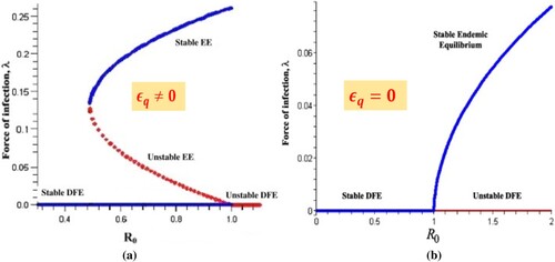${ϵ}_q=0$) has no EE whenever $R_0<1$ (please refer Figure 2(b)). Furthermore, in the model (1(1) $\begin{array}{rl}\frac{\mathrm{d}{S}_u}{\mathrm{d}t}& =\mathrm{\Lambda }-\lambda S_u-\mathrm{d}{S}_u-q{S}_u+\zeta S_q,\\ \frac{\mathrm{d}{S}_q}{\mathrm{d}t}& =q{S}_u+(1-p)\lambda S_u-({ϵ}_q\lambda +\zeta +d)S_q,\\ \frac{\mathrm{d}E}{\mathrm{d}t}& =p\lambda S_u+{ϵ}_q\lambda S_q-(\alpha +d)E,\\ \frac{\mathrm{d}{I}_a}{\mathrm{d}t}& =p_1\alpha E-({\delta }_1+{\varphi }_1+{\gamma }_1+d)I_a,\\ \frac{\mathrm{d}I}{\mathrm{d}t}& =p_2\alpha E-({\delta }_2+{\varphi }_2+{\gamma }_2+d)I,\\ \frac{\mathrm{d}{I}_h}{\mathrm{d}t}& =(1-p_1-p_2)\alpha E+{\varphi }_1{I}_a+{\varphi }_{2}I-({\delta }_3+{\gamma }_3+d)I_h,\\ \frac{\mathrm{d}R}{\mathrm{d}t}& ={\gamma }_1{I}_a+{\gamma }_{2}I+{\gamma }_3{I}_h-\mathrm{d}R,\end{array}$(1) ), the perfect quarantine prevents backward bifurcation (because backward bifurcation requires the existence of at least two endemic equilibria when $R_0\le 1$) [30, 37]. It should also be mentioned that in the scenario that susceptible persons are quarantined but do not become infected during the quarantine, (i.e.${ϵ}_q=0$), the bifurcation coefficient a (given in (13(13) $\begin{array}{rl}a& =\sum _{k,i,j=1}^n{\omega }_k{v}_i{v}_j\frac{{\mathrm{\partial }}^2{f}_k}{\mathrm{\partial }{x}_i\mathrm{\partial }{x}_j}(P^0,{\beta }^{\ast }),\\ & =2v_3^2{\omega }_3\frac{(d+\alpha )}{\mathrm{\Lambda }}(\frac{(d+\alpha )(p-{ϵ}_q)(q{ϵ}_q-(d+\zeta )(1-p))}{(\mathrm{d}p+q{ϵ}_q+p\zeta {)}^2}-(a_{11}+a_{22})),\\ b& =\sum _{k,i=1}^n{\omega }_k{v}_i\frac{{\mathrm{\partial }}^2{f}_k}{\mathrm{\partial }{x}_i\mathrm{\partial }\beta }(P^0,{\beta }^{\ast })={\omega }_3{v}_3\frac{(d+\alpha )}{{\beta }^{\ast }}>0,\end{array}$(13) )) takes the following form $a=-2v_3^2{\omega }_3\frac{(d+\alpha )}{\mathrm{\Lambda }}(\frac{(d+\alpha )(1-p)}{p(d+\zeta )}+(a_{11}+a_{22})).$ Since, $a_{11}>0$ and $a_{22}>0$, a<0, in this case, it follows from Theorem 4.1 of [21] that the model (1(1) $\begin{array}{rl}\frac{\mathrm{d}{S}_u}{\mathrm{d}t}& =\mathrm{\Lambda }-\lambda S_u-\mathrm{d}{S}_u-q{S}_u+\zeta S_q,\\ \frac{\mathrm{d}{S}_q}{\mathrm{d}t}& =q{S}_u+(1-p)\lambda S_u-({ϵ}_q\lambda +\zeta +d)S_q,\\ \frac{\mathrm{d}E}{\mathrm{d}t}& =p\lambda S_u+{ϵ}_q\lambda S_q-(\alpha +d)E,\\ \frac{\mathrm{d}{I}_a}{\mathrm{d}t}& =p_1\alpha E-({\delta }_1+{\varphi }_1+{\gamma }_1+d)I_a,\\ \frac{\mathrm{d}I}{\mathrm{d}t}& =p_2\alpha E-({\delta }_2+{\varphi }_2+{\gamma }_2+d)I,\\ \frac{\mathrm{d}{I}_h}{\mathrm{d}t}& =(1-p_1-p_2)\alpha E+{\varphi }_1{I}_a+{\varphi }_{2}I-({\delta }_3+{\gamma }_3+d)I_h,\\ \frac{\mathrm{d}R}{\mathrm{d}t}& ={\gamma }_1{I}_a+{\gamma }_{2}I+{\gamma }_3{I}_h-\mathrm{d}R,\end{array}$(1) ) does not undergoes to backward bifurcation when ${ϵ}_q=0$. In other words, this research demonstrates that backward bifurcation phenomena for the model (1(1) $\begin{array}{rl}\frac{\mathrm{d}{S}_u}{\mathrm{d}t}& =\mathrm{\Lambda }-\lambda S_u-\mathrm{d}{S}_u-q{S}_u+\zeta S_q,\\ \frac{\mathrm{d}{S}_q}{\mathrm{d}t}& =q{S}_u+(1-p)\lambda S_u-({ϵ}_q\lambda +\zeta +d)S_q,\\ \frac{\mathrm{d}E}{\mathrm{d}t}& =p\lambda S_u+{ϵ}_q\lambda S_q-(\alpha +d)E,\\ \frac{\mathrm{d}{I}_a}{\mathrm{d}t}& =p_1\alpha E-({\delta }_1+{\varphi }_1+{\gamma }_1+d)I_a,\\ \frac{\mathrm{d}I}{\mathrm{d}t}& =p_2\alpha E-({\delta }_2+{\varphi }_2+{\gamma }_2+d)I,\\ \frac{\mathrm{d}{I}_h}{\mathrm{d}t}& =(1-p_1-p_2)\alpha E+{\varphi }_1{I}_a+{\varphi }_{2}I-({\delta }_3+{\gamma }_3+d)I_h,\\ \frac{\mathrm{d}R}{\mathrm{d}t}& ={\gamma }_1{I}_a+{\gamma }_{2}I+{\gamma }_3{I}_h-\mathrm{d}R,\end{array}$(1) ) trait is caused by the infection of susceptible individuals in quarantine. This result is in line with Theorem 3.2. The graphical representation of bifurcation analysis for model system is depicted in Figure 2.

Figure 2. The figure shows the bifurcation analysis discussed in Section 3.4.1. (a) backward bifurcation when imperfect quarantine is implemented $({ϵ}_q\ne 0)$ and (b) backward bifurcation when perfect quarantine is implemented $({ϵ}_q=0)$.

3.5. Threshold dynamics of the basic reproduction number

Here, we demonstrate the threshold dynamics of the basic reproduction number concerning control parameters related to quarantine and isolation to see how much control measure is required for its positive effect. A threshold analysis of the parameters related to quarantine $(\zeta \mathrm{and}q)$ and isolation/hospitalization of asymptomatic and symptomatic infected individuals (${\varphi }_1$ and ${\varphi }_2$) are investigated by calculating partial derivatives of $R_0$ (which is given by Equation (4(4) $R_0=R_0^I+R_0^{I_a}+R_0^{I_h},$(4) )) with respect to these parameters. Therefore, we have (14) $\frac{\mathrm{\partial }{R}_0}{\mathrm{\partial }\zeta }=\frac{\begin{array}{c}q\alpha \beta (1-p_M{ϵ}_M)(p-{ϵ}_q)\\ (K_2{K}_3{p}_1{\psi }_a+K_1{K}_3{p}_2+(K_2{p}_1{\varphi }_1+K_1{p}_2{\varphi }_2+K_1{K}_2(1-p_1-p_2)){\psi }_h)\end{array}}{K_1{K}_2{K}_3(d+\alpha ){(d+q+\zeta )}^2}.$(14) From Equation (14(14) $\frac{\mathrm{\partial }{R}_0}{\mathrm{\partial }\zeta }=\frac{\begin{array}{c}q\alpha \beta (1-p_M{ϵ}_M)(p-{ϵ}_q)\\ (K_2{K}_3{p}_1{\psi }_a+K_1{K}_3{p}_2+(K_2{p}_1{\varphi }_1+K_1{p}_2{\varphi }_2+K_1{K}_2(1-p_1-p_2)){\psi }_h)\end{array}}{K_1{K}_2{K}_3(d+\alpha ){(d+q+\zeta )}^2}.$(14) ), it is obvious that $\frac{\mathrm{\partial }{R}_0}{\mathrm{\partial }\zeta }>0(<0)$ when $p-{ϵ}_q>0(p-{ϵ}_q<0).$ Therefore, if $p>{ϵ}_q$ then we have that the $R_0$ decreases as value of ζ decreases ($\text{days of quarantine }(\frac{1}{\zeta })$ increases). If we decrease the values of ζ $(\text{increases the days of}\text{quarantine }(\frac{1}{\zeta }))$ then basic reproduction number increases when $p<{ϵ}_q$. Therefore, we obtain that $p>{ϵ}_q$ is the necessary condition for the successful quarantine. (15) $\frac{\mathrm{\partial }{R}_0}{\mathrm{\partial }q}=-\frac{\begin{array}{c}q\alpha \beta (1-p_M{ϵ}_M)(p-{ϵ}_q)\\ (K_2{K}_3{p}_1{\psi }_a+K_1{K}_3{p}_2+(K_2{p}_1{\varphi }_1+K_1{p}_2{\varphi }_2+K_1{K}_2(1-p_1-p_2)){\psi }_h)\end{array}}{K_1{K}_2{K}_3(d+\alpha ){(d+q+\zeta )}^2}.$(15) From Equation (15(15) $\frac{\mathrm{\partial }{R}_0}{\mathrm{\partial }q}=-\frac{\begin{array}{c}q\alpha \beta (1-p_M{ϵ}_M)(p-{ϵ}_q)\\ (K_2{K}_3{p}_1{\psi }_a+K_1{K}_3{p}_2+(K_2{p}_1{\varphi }_1+K_1{p}_2{\varphi }_2+K_1{K}_2(1-p_1-p_2)){\psi }_h)\end{array}}{K_1{K}_2{K}_3(d+\alpha ){(d+q+\zeta )}^2}.$(15) ), we can easily observe that $\frac{\mathrm{\partial }{R}_0}{\mathrm{\partial }q}<0(>0)$ when $p-{ϵ}_q>0(p-{ϵ}_q<0).$ Therefore, if $p>{ϵ}_q$ then we have that the $R_0$ decreases as value of q (quarantine rate) increase. If we increase the values of q then $R_0$ increases when $p<{ϵ}_q$. Hence, by Equations (14(14) $\frac{\mathrm{\partial }{R}_0}{\mathrm{\partial }\zeta }=\frac{\begin{array}{c}q\alpha \beta (1-p_M{ϵ}_M)(p-{ϵ}_q)\\ (K_2{K}_3{p}_1{\psi }_a+K_1{K}_3{p}_2+(K_2{p}_1{\varphi }_1+K_1{p}_2{\varphi }_2+K_1{K}_2(1-p_1-p_2)){\psi }_h)\end{array}}{K_1{K}_2{K}_3(d+\alpha ){(d+q+\zeta )}^2}.$(14) ) and (15(15) $\frac{\mathrm{\partial }{R}_0}{\mathrm{\partial }q}=-\frac{\begin{array}{c}q\alpha \beta (1-p_M{ϵ}_M)(p-{ϵ}_q)\\ (K_2{K}_3{p}_1{\psi }_a+K_1{K}_3{p}_2+(K_2{p}_1{\varphi }_1+K_1{p}_2{\varphi }_2+K_1{K}_2(1-p_1-p_2)){\psi }_h)\end{array}}{K_1{K}_2{K}_3(d+\alpha ){(d+q+\zeta )}^2}.$(15) ), we conclude that quarantine may be harmful for people when the efficacy of quarantine is below than threshold value or infection transmission rate in quarantine is higher than the critical value ${ϵ}_q^{\ast }({ϵ}_q^{\ast }=p).$ Further, we determine the dynamic of $R_0$ with respect to isolation process. Here (16) $\frac{\mathrm{\partial }{R}_0}{\mathrm{\partial }{\varphi }_1}=-\frac{p_1\alpha \beta (1-p_M{ϵ}_M)(\mathrm{d}p+q{ϵ}_q+p\zeta )((d+{\gamma }_3+{\delta }_3){\psi }_a-(d+{\gamma }_1+{\delta }_1){\psi }_h)}{K_1^2{K}_3(d+\alpha )(d+q+\zeta )}.$(16) By Equation (16(16) $\frac{\mathrm{\partial }{R}_0}{\mathrm{\partial }{\varphi }_1}=-\frac{p_1\alpha \beta (1-p_M{ϵ}_M)(\mathrm{d}p+q{ϵ}_q+p\zeta )((d+{\gamma }_3+{\delta }_3){\psi }_a-(d+{\gamma }_1+{\delta }_1){\psi }_h)}{K_1^2{K}_3(d+\alpha )(d+q+\zeta )}.$(16) ), we have that $\frac{\mathrm{\partial }{R}_0}{\mathrm{\partial }{\varphi }_1}<0(>0)$ for ${\psi }_h<\frac{(d+{\gamma }_3+{\delta }_3){\psi }_a}{d+{\gamma }_1+{\delta }_1}({\psi }_h>\frac{(d+{\gamma }_3+{\delta }_3){\psi }_a}{d+{\gamma }_1+{\delta }_1}).$ Precisely, hospitalization/isolation of asymptomatic infected individuals have positive impact on the basic reproduction number when infectiousness of isolated infected individuals is below than a threshold value ${\psi }_{h1}^{\ast }$ $({\psi }_{h1}^{\ast }=\frac{(d+{\gamma }_3+{\delta }_3){\psi }_a}{d+{\gamma }_1+{\delta }_1}).$ Similarly, we have (17) $\frac{\mathrm{\partial }{R}_0}{\mathrm{\partial }{\varphi }_2}=-\frac{p_2\alpha \beta (1-p_M{ϵ}_M)(\mathrm{d}p+q{ϵ}_q+p\zeta )((d+{\gamma }_3+{\delta }_3)-(d+{\gamma }_2+{\delta }_2){\psi }_h)}{K_2^2{K}_3(d+\alpha )(d+q+\zeta )}.$(17) By Equation (17(17) $\frac{\mathrm{\partial }{R}_0}{\mathrm{\partial }{\varphi }_2}=-\frac{p_2\alpha \beta (1-p_M{ϵ}_M)(\mathrm{d}p+q{ϵ}_q+p\zeta )((d+{\gamma }_3+{\delta }_3)-(d+{\gamma }_2+{\delta }_2){\psi }_h)}{K_2^2{K}_3(d+\alpha )(d+q+\zeta )}.$(17) ), we have that $\frac{\mathrm{\partial }{R}_0}{\mathrm{\partial }{\varphi }_2}<0(>0)$ for ${\psi }_h<\frac{d+{\gamma }_3+{\delta }_3}{d+{\gamma }_2+{\delta }_2}({\psi }_h>\frac{d+{\gamma }_3+{\delta }_3}{d+{\gamma }_2+{\delta }_2}).$ Therefore, we have a threshold value $({\psi }_{h2}^{\ast })$ of infectiousness of isolated infected individuals to successful isolation of symptomatic infected individuals where $({\psi }_{h2}^{\ast }=\frac{d+{\gamma }_3+{\delta }_3}{d+{\gamma }_2+{\delta }_2}).$ Furthermore, From Equations (16(16) $\frac{\mathrm{\partial }{R}_0}{\mathrm{\partial }{\varphi }_1}=-\frac{p_1\alpha \beta (1-p_M{ϵ}_M)(\mathrm{d}p+q{ϵ}_q+p\zeta )((d+{\gamma }_3+{\delta }_3){\psi }_a-(d+{\gamma }_1+{\delta }_1){\psi }_h)}{K_1^2{K}_3(d+\alpha )(d+q+\zeta )}.$(16) ) and (17(17) $\frac{\mathrm{\partial }{R}_0}{\mathrm{\partial }{\varphi }_2}=-\frac{p_2\alpha \beta (1-p_M{ϵ}_M)(\mathrm{d}p+q{ϵ}_q+p\zeta )((d+{\gamma }_3+{\delta }_3)-(d+{\gamma }_2+{\delta }_2){\psi }_h)}{K_2^2{K}_3(d+\alpha )(d+q+\zeta )}.$(17) ), we conclude that the hospitalization/isolation of infected individuals will help in reducing the disease burden in community when infectiousness of isolated infected individuals is below than its critical value ${\psi }_h^{\ast }$ $({\psi }_h^{\ast }=min\{{\psi }_{h1}^{\ast }{\psi }_{h2}^{\ast }\}).$ The numerical validation of discussion related to the threshold dynamics of basic reproduction number has been shown in Figure 9.

4. Numerical simulations

In this section, we estimate some of the model parameters using actual COVID-19 data for India, as well as numerically validate the theoretical findings. The impact of various control parameters on COVID-19 transmission dynamics in India is also discussed.

4.1. Estimation of the model parameters

We calibrate the model system (1(1) $\begin{array}{rl}\frac{\mathrm{d}{S}_u}{\mathrm{d}t}& =\mathrm{\Lambda }-\lambda S_u-\mathrm{d}{S}_u-q{S}_u+\zeta S_q,\\ \frac{\mathrm{d}{S}_q}{\mathrm{d}t}& =q{S}_u+(1-p)\lambda S_u-({ϵ}_q\lambda +\zeta +d)S_q,\\ \frac{\mathrm{d}E}{\mathrm{d}t}& =p\lambda S_u+{ϵ}_q\lambda S_q-(\alpha +d)E,\\ \frac{\mathrm{d}{I}_a}{\mathrm{d}t}& =p_1\alpha E-({\delta }_1+{\varphi }_1+{\gamma }_1+d)I_a,\\ \frac{\mathrm{d}I}{\mathrm{d}t}& =p_2\alpha E-({\delta }_2+{\varphi }_2+{\gamma }_2+d)I,\\ \frac{\mathrm{d}{I}_h}{\mathrm{d}t}& =(1-p_1-p_2)\alpha E+{\varphi }_1{I}_a+{\varphi }_{2}I-({\delta }_3+{\gamma }_3+d)I_h,\\ \frac{\mathrm{d}R}{\mathrm{d}t}& ={\gamma }_1{I}_a+{\gamma }_{2}I+{\gamma }_3{I}_h-\mathrm{d}R,\end{array}$(1) ) to study the cumulative confirmed cases of COVID-19 in India. The actual data of cumulative cases of COVID-19 in India are collected for the period September 1, 2020–December 31, 2020, from the official websites of the WHO (World Health Organization) [72] and the Coronavirus Worldometer [74]. To begin, we use accessible COVID-19 information, important data, and source materials from published articles to measure the baseline values of the some of the model parameters. We omit the new recruitment rate in susceptible persons and natural death rates of all people (demographics) due to short duration of the study of COVID-19 outbreaks compared to the length of the life span, i.e. we assume $\mathrm{\Lambda }=0$ and d = 0. Since the quarantine period of 14 days is suggested for suspected people of being exposed to COVID-19 by WHO [71, 73]. As a result, we define $\zeta =\frac{1}{14}$ per day as the rate at which quarantined people relapse into the non-quarantined susceptible class. Further, some research have estimated the incubation for COVID-19 to be 5–6 days [45], and 2–14 days with roughly $97.5\mathrm{\%}$ of infected persons presenting the symptoms with 11.5 days after receiving infection [27, 43]. Therefore, we set the average incubation period of 5.2 days. i.e. $\alpha =\frac{1}{5.2}$ per day.

In [32, 82], the authors suggested an infectious period of 10 days for the COVID-19 and the average period after the COVID-19 patients will be released from the hospital to be 8 days. Therefore, we take the recovery rate for asymptomatic-infectious individuals, symptomatic-infectious individuals, and hospitalized infectious individuals, ${\gamma }_1={\gamma }_2=\frac{1}{10}$ per day and ${\gamma }_3=\frac{1}{8}$ per day, respectively. It is expected that there is a small lag time (of around 5 days) between the development of COVID-19 symptoms in infected persons and hospitalization, similar to Ferguson et al. [32]. As a result, we put the symptomatically infectious people' hospitalization rate as ${\varphi }_2=\frac{1}{5}$ per day. According to certain research, $80\mathrm{\%}$ of COVID-19 individuals have little or no symptoms, $14\mathrm{\%}$ have severe symptoms, and $6\mathrm{\%}$ have dangerously severe symptoms needing ICU beds in hospitals. [4, 31]. As a result, we use $p_2=0.2$ and suppose that $40\mathrm{\%}$ of instances with no or minor symptoms are asymptomatic persons. i.e. $p_1=\mathrm{0.4.}$ Further, Li et al. [46] estimated the modification parameters for the relative infectiousness of asymptomatic individuals to be between 0.42 and 0.55. Hence, we set ${\psi }_a=0.49$ and assume ${\psi }_h=\mathrm{0.35.}$ The parameter ${ϵ}_q=0.5$ is used to estimate the effectiveness of quarantine in infection prevention throughout quarantined.

Based on the results of several clinical investigations, we also established the efficiency of face masks. In cystic fibrosis patients, for example, Driessche et al. [28] found that surgical masks suppressed Pseudomonas aeruginosa infected aerosols produced by sneezing through over $80\mathrm{\%}$. Surgical masks lowered colony-forming unit (CFU) count by over 90 percent, according to a study by Stockwell et al. [63]. As a result, both research in [28, 63] show that N95 masks are much more important in protecting against infections. Similarly, a study published by authors [68] showed that homemade fabric masks exhibited the inward efficiency of $58\mathrm{\%}$–$77\mathrm{\%}$ after a three-hour period of usage, but surgical and N95 equivalent masks had inward efficiency of $72\mathrm{\%}$–$85\mathrm{\%}$ and $98\mathrm{\%}$–$99\mathrm{\%}$. Nevertheless, the authors of [29] estimated inward mask efficacy to be anywhere from $20\mathrm{\%}$ to $80\mathrm{\%}$ for cotton masks, at least $50\mathrm{\%}$ for well-crafted, tightly fitting masks manufactured by ideal material, $70\mathrm{\%}$ to $90\mathrm{\%}$ for surgical masks, and over $95\mathrm{\%}$ for correctly worn $N95$ masks. Based on the above literature survey, we set ${ϵ}_M=0.6$. The numerical values of model parameters are shown in Table 4 that are used in simulations of model system (1(1) $\begin{array}{rl}\frac{\mathrm{d}{S}_u}{\mathrm{d}t}& =\mathrm{\Lambda }-\lambda S_u-\mathrm{d}{S}_u-q{S}_u+\zeta S_q,\\ \frac{\mathrm{d}{S}_q}{\mathrm{d}t}& =q{S}_u+(1-p)\lambda S_u-({ϵ}_q\lambda +\zeta +d)S_q,\\ \frac{\mathrm{d}E}{\mathrm{d}t}& =p\lambda S_u+{ϵ}_q\lambda S_q-(\alpha +d)E,\\ \frac{\mathrm{d}{I}_a}{\mathrm{d}t}& =p_1\alpha E-({\delta }_1+{\varphi }_1+{\gamma }_1+d)I_a,\\ \frac{\mathrm{d}I}{\mathrm{d}t}& =p_2\alpha E-({\delta }_2+{\varphi }_2+{\gamma }_2+d)I,\\ \frac{\mathrm{d}{I}_h}{\mathrm{d}t}& =(1-p_1-p_2)\alpha E+{\varphi }_1{I}_a+{\varphi }_{2}I-({\delta }_3+{\gamma }_3+d)I_h,\\ \frac{\mathrm{d}R}{\mathrm{d}t}& ={\gamma }_1{I}_a+{\gamma }_{2}I+{\gamma }_3{I}_h-\mathrm{d}R,\end{array}$(1) ). The cumulative cases $(C(t))$ for model system (1(1) $\begin{array}{rl}\frac{\mathrm{d}{S}_u}{\mathrm{d}t}& =\mathrm{\Lambda }-\lambda S_u-\mathrm{d}{S}_u-q{S}_u+\zeta S_q,\\ \frac{\mathrm{d}{S}_q}{\mathrm{d}t}& =q{S}_u+(1-p)\lambda S_u-({ϵ}_q\lambda +\zeta +d)S_q,\\ \frac{\mathrm{d}E}{\mathrm{d}t}& =p\lambda S_u+{ϵ}_q\lambda S_q-(\alpha +d)E,\\ \frac{\mathrm{d}{I}_a}{\mathrm{d}t}& =p_1\alpha E-({\delta }_1+{\varphi }_1+{\gamma }_1+d)I_a,\\ \frac{\mathrm{d}I}{\mathrm{d}t}& =p_2\alpha E-({\delta }_2+{\varphi }_2+{\gamma }_2+d)I,\\ \frac{\mathrm{d}{I}_h}{\mathrm{d}t}& =(1-p_1-p_2)\alpha E+{\varphi }_1{I}_a+{\varphi }_{2}I-({\delta }_3+{\gamma }_3+d)I_h,\\ \frac{\mathrm{d}R}{\mathrm{d}t}& ={\gamma }_1{I}_a+{\gamma }_{2}I+{\gamma }_3{I}_h-\mathrm{d}R,\end{array}$(1) ) is computed by the following equation: (18) $\frac{\mathrm{d}C(t)}{\mathrm{d}t}=\alpha E(t).$(18) We postulate and take several parameters from published studies (Table 4) except β and $p_M$, and initial conditions for the system variables are the same as in Table 3. We apply extended Markov-chain Monte-Carlo (MCMC) simulations based on the adaptive combination delayed Rejection and Adaptive Metropolis (DRAM) technique to determine the values of parameters β and $p_M$ [36, 40]. We estimate the model parameters of β and $p_M$ with Monte -- Carlo chain distribution and the temporal dynamics of cumulative cases using 100,000 sample realizations, and compare with actual data of confirmed COVID-19 cases displayed in Figure 3. The mean values, standard deviation, and Geweke values for β and $p_M$ are also computed and displayed in Table 2.

Figure 3. (a) The histogram of MCMC chain for parameters β and $p_M$ with 100, 000 sample realizations. (b) Fitting results of reported cases for India to the model output.

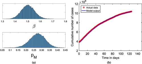
Table 2. The estimated values of model parameters $\beta \mathrm{and}{p}_M$ with its $95\mathrm{\%}$ confidence interval obtained via MCMC method.

Parameters	Mean values	Standard deviations	$95\mathrm{\%}$ CI	Geweke values
β	1.5030	0.0524	$(1.3982,1.6078)$	0.9972
$p_M$	0.2728	0.0486	$(0.1756,0.3700)$	0.9958

Table 3. Initial conditions for the system (1(1) $\begin{array}{rl}\frac{\mathrm{d}{S}_u}{\mathrm{d}t}& =\mathrm{\Lambda }-\lambda S_u-\mathrm{d}{S}_u-q{S}_u+\zeta S_q,\\ \frac{\mathrm{d}{S}_q}{\mathrm{d}t}& =q{S}_u+(1-p)\lambda S_u-({ϵ}_q\lambda +\zeta +d)S_q,\\ \frac{\mathrm{d}E}{\mathrm{d}t}& =p\lambda S_u+{ϵ}_q\lambda S_q-(\alpha +d)E,\\ \frac{\mathrm{d}{I}_a}{\mathrm{d}t}& =p_1\alpha E-({\delta }_1+{\varphi }_1+{\gamma }_1+d)I_a,\\ \frac{\mathrm{d}I}{\mathrm{d}t}& =p_2\alpha E-({\delta }_2+{\varphi }_2+{\gamma }_2+d)I,\\ \frac{\mathrm{d}{I}_h}{\mathrm{d}t}& =(1-p_1-p_2)\alpha E+{\varphi }_1{I}_a+{\varphi }_{2}I-({\delta }_3+{\gamma }_3+d)I_h,\\ \frac{\mathrm{d}R}{\mathrm{d}t}& ={\gamma }_1{I}_a+{\gamma }_{2}I+{\gamma }_3{I}_h-\mathrm{d}R,\end{array}$(1) ).

$S_u(0)$	$S_q(0)$	$E(0)$	$I_a(0)$	$I(0)$	$I_h(0)$	$R(0)$
$1.35\times {10}^9$	$1.15\times {10}^7$	$2.76\times {10}^6$	$6.6\times {10}^5$	$9.42\times {10}^4$	$1.89\times {10}^5$	$2.96\times {10}^6$

Table 4. The table contains numerical values of model parameters used for transmission dynamics of system (1(1) $\begin{array}{rl}\frac{\mathrm{d}{S}_u}{\mathrm{d}t}& =\mathrm{\Lambda }-\lambda S_u-\mathrm{d}{S}_u-q{S}_u+\zeta S_q,\\ \frac{\mathrm{d}{S}_q}{\mathrm{d}t}& =q{S}_u+(1-p)\lambda S_u-({ϵ}_q\lambda +\zeta +d)S_q,\\ \frac{\mathrm{d}E}{\mathrm{d}t}& =p\lambda S_u+{ϵ}_q\lambda S_q-(\alpha +d)E,\\ \frac{\mathrm{d}{I}_a}{\mathrm{d}t}& =p_1\alpha E-({\delta }_1+{\varphi }_1+{\gamma }_1+d)I_a,\\ \frac{\mathrm{d}I}{\mathrm{d}t}& =p_2\alpha E-({\delta }_2+{\varphi }_2+{\gamma }_2+d)I,\\ \frac{\mathrm{d}{I}_h}{\mathrm{d}t}& =(1-p_1-p_2)\alpha E+{\varphi }_1{I}_a+{\varphi }_{2}I-({\delta }_3+{\gamma }_3+d)I_h,\\ \frac{\mathrm{d}R}{\mathrm{d}t}& ={\gamma }_1{I}_a+{\gamma }_{2}I+{\gamma }_3{I}_h-\mathrm{d}R,\end{array}$(1) ) for COVID-19 in India.

Parameters	Numerical value	Units	References
Γ	0	day${}^{-1}$	Assumed
${ϵ}_M$	0.6		[28, 29, 63, 68]
${\psi }_a$	0.49		[46]
${\psi }_h$	0.35		assumed
${ϵ}_h$	0.2		assumed
d	0	day${}^{-1}$	assumed
q	0.25		assumed
ζ	$\frac{1}{14}$	day${}^{-1}$	[71, 73]
p	0.36651		assumed
${ϵ}_q$	0.2		assumed
α	0.1980	day${}^{-1}$	[45]
$p_1$	0.4		[4, 31]
$p_2$	0.2		[4, 31]
${\delta }_1$	0.0019	day${}^{-1}$	assumed
${\delta }_2$	0.0019	day${}^{-1}$	assumed
${\delta }_3$	0.0018	day${}^{-1}$	assumed
${\gamma }_1$	0.1	day${}^{-1}$	[32, 82]
${\gamma }_2$	0.1	day${}^{-1}$	[32, 82]
${\gamma }_3$	0.125	day${}^{-1}$	[32, 82]
${\varphi }_1$	0.456	day${}^{-1}$	assumed
${\varphi }_2$	0.2	day${}^{-1}$	[32]

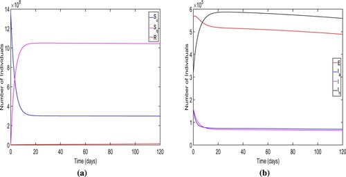
4.2. Numerical validation for local stability of equilibria

Here, we illustrate the numerical validation the stability results related to equilibria discussed in Sections 3.3 and 3.4.

Firstly, we verify the local stability of DFE $(P^0)$ and choose $\beta =0.951,{ϵ}_q=0.05$ and other parametric values are taken from Tables 2 and 4. For these parametric values, we obtain the $R_0=0.4951<1$ and DFE $P^0=(30\times {10}^7,10.5\times {10}^8,0,0,0,0,0).$ We also display the solution trajectories of the system (1(1) $\begin{array}{rl}\frac{\mathrm{d}{S}_u}{\mathrm{d}t}& =\mathrm{\Lambda }-\lambda S_u-\mathrm{d}{S}_u-q{S}_u+\zeta S_q,\\ \frac{\mathrm{d}{S}_q}{\mathrm{d}t}& =q{S}_u+(1-p)\lambda S_u-({ϵ}_q\lambda +\zeta +d)S_q,\\ \frac{\mathrm{d}E}{\mathrm{d}t}& =p\lambda S_u+{ϵ}_q\lambda S_q-(\alpha +d)E,\\ \frac{\mathrm{d}{I}_a}{\mathrm{d}t}& =p_1\alpha E-({\delta }_1+{\varphi }_1+{\gamma }_1+d)I_a,\\ \frac{\mathrm{d}I}{\mathrm{d}t}& =p_2\alpha E-({\delta }_2+{\varphi }_2+{\gamma }_2+d)I,\\ \frac{\mathrm{d}{I}_h}{\mathrm{d}t}& =(1-p_1-p_2)\alpha E+{\varphi }_1{I}_a+{\varphi }_{2}I-({\delta }_3+{\gamma }_3+d)I_h,\\ \frac{\mathrm{d}R}{\mathrm{d}t}& ={\gamma }_1{I}_a+{\gamma }_{2}I+{\gamma }_3{I}_h-\mathrm{d}R,\end{array}$(1) ) across time and can see that both unquarantined and quarantined susceptible individuals eventually settle to a positive level. (refer Figure 4(a)). In Figure 4(b), the endemic solutions trajectories for all diseased compartments eventually converge to zero. Thus, the solutions of the model system (1(1) $\begin{array}{rl}\frac{\mathrm{d}{S}_u}{\mathrm{d}t}& =\mathrm{\Lambda }-\lambda S_u-\mathrm{d}{S}_u-q{S}_u+\zeta S_q,\\ \frac{\mathrm{d}{S}_q}{\mathrm{d}t}& =q{S}_u+(1-p)\lambda S_u-({ϵ}_q\lambda +\zeta +d)S_q,\\ \frac{\mathrm{d}E}{\mathrm{d}t}& =p\lambda S_u+{ϵ}_q\lambda S_q-(\alpha +d)E,\\ \frac{\mathrm{d}{I}_a}{\mathrm{d}t}& =p_1\alpha E-({\delta }_1+{\varphi }_1+{\gamma }_1+d)I_a,\\ \frac{\mathrm{d}I}{\mathrm{d}t}& =p_2\alpha E-({\delta }_2+{\varphi }_2+{\gamma }_2+d)I,\\ \frac{\mathrm{d}{I}_h}{\mathrm{d}t}& =(1-p_1-p_2)\alpha E+{\varphi }_1{I}_a+{\varphi }_{2}I-({\delta }_3+{\gamma }_3+d)I_h,\\ \frac{\mathrm{d}R}{\mathrm{d}t}& ={\gamma }_1{I}_a+{\gamma }_{2}I+{\gamma }_3{I}_h-\mathrm{d}R,\end{array}$(1) ) approach $P^0$. Consequently, Figure 4 ensure the local stability of DFE $P^0$.

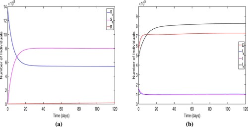
For Figure 5, we choose $\beta =0.951,{ϵ}_q=0.35$ and other parametric values are taken from Tables 2 and  4. For this set of numerical values of model parameters, we find the $R_0=0.9529<1$ and two endemic equilibria along with a disease free equilibrium. One of the endemic equilibrium for the system (1(1) $\begin{array}{rl}\frac{\mathrm{d}{S}_u}{\mathrm{d}t}& =\mathrm{\Lambda }-\lambda S_u-\mathrm{d}{S}_u-q{S}_u+\zeta S_q,\\ \frac{\mathrm{d}{S}_q}{\mathrm{d}t}& =q{S}_u+(1-p)\lambda S_u-({ϵ}_q\lambda +\zeta +d)S_q,\\ \frac{\mathrm{d}E}{\mathrm{d}t}& =p\lambda S_u+{ϵ}_q\lambda S_q-(\alpha +d)E,\\ \frac{\mathrm{d}{I}_a}{\mathrm{d}t}& =p_1\alpha E-({\delta }_1+{\varphi }_1+{\gamma }_1+d)I_a,\\ \frac{\mathrm{d}I}{\mathrm{d}t}& =p_2\alpha E-({\delta }_2+{\varphi }_2+{\gamma }_2+d)I,\\ \frac{\mathrm{d}{I}_h}{\mathrm{d}t}& =(1-p_1-p_2)\alpha E+{\varphi }_1{I}_a+{\varphi }_{2}I-({\delta }_3+{\gamma }_3+d)I_h,\\ \frac{\mathrm{d}R}{\mathrm{d}t}& ={\gamma }_1{I}_a+{\gamma }_{2}I+{\gamma }_3{I}_h-\mathrm{d}R,\end{array}$(1) ) is given by $P_1^{\ast }=(2.99\times {10}^8,1.04\times {10}^9,1.06\times {10}^5,1.55\times {10}^4,1.46\times {10}^4,1.37\times {10}^5,9.04\times {10}^6)$. Further, we plot the time series of the solution set of the model system (1(1) $\begin{array}{rl}\frac{\mathrm{d}{S}_u}{\mathrm{d}t}& =\mathrm{\Lambda }-\lambda S_u-\mathrm{d}{S}_u-q{S}_u+\zeta S_q,\\ \frac{\mathrm{d}{S}_q}{\mathrm{d}t}& =q{S}_u+(1-p)\lambda S_u-({ϵ}_q\lambda +\zeta +d)S_q,\\ \frac{\mathrm{d}E}{\mathrm{d}t}& =p\lambda S_u+{ϵ}_q\lambda S_q-(\alpha +d)E,\\ \frac{\mathrm{d}{I}_a}{\mathrm{d}t}& =p_1\alpha E-({\delta }_1+{\varphi }_1+{\gamma }_1+d)I_a,\\ \frac{\mathrm{d}I}{\mathrm{d}t}& =p_2\alpha E-({\delta }_2+{\varphi }_2+{\gamma }_2+d)I,\\ \frac{\mathrm{d}{I}_h}{\mathrm{d}t}& =(1-p_1-p_2)\alpha E+{\varphi }_1{I}_a+{\varphi }_{2}I-({\delta }_3+{\gamma }_3+d)I_h,\\ \frac{\mathrm{d}R}{\mathrm{d}t}& ={\gamma }_1{I}_a+{\gamma }_{2}I+{\gamma }_3{I}_h-\mathrm{d}R,\end{array}$(1) ) for considered parametric values (Figure 5). In this figure, we notice that the solution trajectories converge to the endemic equilibrium $P_1^{\ast }$. Thus, the figure ensure the local stability of endemic equilibrium $P_1^{\ast }$ for $R_0<1.$ From Figures 4 and 5, we conclude that for high efficacy of quarantine (for lower value of ${ϵ}_q$), only the disease free equilibrium is stable point when $R_0<1$ but for low efficacy of quarantine (for higher value of ${ϵ}_q$), there are two stable equilibria (DFE $P^0$ and endemic equilibrium $P_1^{\ast }$) when $R_0<1.$ Therefore, we show that the model system (1(1) $\begin{array}{rl}\frac{\mathrm{d}{S}_u}{\mathrm{d}t}& =\mathrm{\Lambda }-\lambda S_u-\mathrm{d}{S}_u-q{S}_u+\zeta S_q,\\ \frac{\mathrm{d}{S}_q}{\mathrm{d}t}& =q{S}_u+(1-p)\lambda S_u-({ϵ}_q\lambda +\zeta +d)S_q,\\ \frac{\mathrm{d}E}{\mathrm{d}t}& =p\lambda S_u+{ϵ}_q\lambda S_q-(\alpha +d)E,\\ \frac{\mathrm{d}{I}_a}{\mathrm{d}t}& =p_1\alpha E-({\delta }_1+{\varphi }_1+{\gamma }_1+d)I_a,\\ \frac{\mathrm{d}I}{\mathrm{d}t}& =p_2\alpha E-({\delta }_2+{\varphi }_2+{\gamma }_2+d)I,\\ \frac{\mathrm{d}{I}_h}{\mathrm{d}t}& =(1-p_1-p_2)\alpha E+{\varphi }_1{I}_a+{\varphi }_{2}I-({\delta }_3+{\gamma }_3+d)I_h,\\ \frac{\mathrm{d}R}{\mathrm{d}t}& ={\gamma }_1{I}_a+{\gamma }_{2}I+{\gamma }_3{I}_h-\mathrm{d}R,\end{array}$(1) ) demonstrates the bistable behaviour for the low efficacy quarantine when $R_0<1.$

To verify the existence and local stability of endemic equilibrium when $R_0>1$, we choose $\beta =1.502,{ϵ}_q=0.2$ and remaining parametric values are same as discussed in Tables 2 and 4. We compute the basic reproduction number $R_0=1.3649$ and a unique endemic equilibrium $P^{\ast }=(5.40\times {10}^8,7.96\times {10}^8,7.27\times {10}^5,1.03\times {10}^5,0.95\times {10}^5,8.26\times {10}^5,1.73\times {10}^7)$ for this set of parametric values. Furthermore, we draw the times series of the solution set of the model system (1(1) $\begin{array}{rl}\frac{\mathrm{d}{S}_u}{\mathrm{d}t}& =\mathrm{\Lambda }-\lambda S_u-\mathrm{d}{S}_u-q{S}_u+\zeta S_q,\\ \frac{\mathrm{d}{S}_q}{\mathrm{d}t}& =q{S}_u+(1-p)\lambda S_u-({ϵ}_q\lambda +\zeta +d)S_q,\\ \frac{\mathrm{d}E}{\mathrm{d}t}& =p\lambda S_u+{ϵ}_q\lambda S_q-(\alpha +d)E,\\ \frac{\mathrm{d}{I}_a}{\mathrm{d}t}& =p_1\alpha E-({\delta }_1+{\varphi }_1+{\gamma }_1+d)I_a,\\ \frac{\mathrm{d}I}{\mathrm{d}t}& =p_2\alpha E-({\delta }_2+{\varphi }_2+{\gamma }_2+d)I,\\ \frac{\mathrm{d}{I}_h}{\mathrm{d}t}& =(1-p_1-p_2)\alpha E+{\varphi }_1{I}_a+{\varphi }_{2}I-({\delta }_3+{\gamma }_3+d)I_h,\\ \frac{\mathrm{d}R}{\mathrm{d}t}& ={\gamma }_1{I}_a+{\gamma }_{2}I+{\gamma }_3{I}_h-\mathrm{d}R,\end{array}$(1) ) and observe that the solutions trajectories approach to the positive level of endemicity (endemic equilibrium $P^{\ast }$) (refer the Figure 6). Thus, we ensure the local stability of endemic equilibrium $P^{\ast }$ when $R_0>1$.

Figure 4. The long-term dynamics of the model system (1(1) $\begin{array}{rl}\frac{\mathrm{d}{S}_u}{\mathrm{d}t}& =\mathrm{\Lambda }-\lambda S_u-\mathrm{d}{S}_u-q{S}_u+\zeta S_q,\\ \frac{\mathrm{d}{S}_q}{\mathrm{d}t}& =q{S}_u+(1-p)\lambda S_u-({ϵ}_q\lambda +\zeta +d)S_q,\\ \frac{\mathrm{d}E}{\mathrm{d}t}& =p\lambda S_u+{ϵ}_q\lambda S_q-(\alpha +d)E,\\ \frac{\mathrm{d}{I}_a}{\mathrm{d}t}& =p_1\alpha E-({\delta }_1+{\varphi }_1+{\gamma }_1+d)I_a,\\ \frac{\mathrm{d}I}{\mathrm{d}t}& =p_2\alpha E-({\delta }_2+{\varphi }_2+{\gamma }_2+d)I,\\ \frac{\mathrm{d}{I}_h}{\mathrm{d}t}& =(1-p_1-p_2)\alpha E+{\varphi }_1{I}_a+{\varphi }_{2}I-({\delta }_3+{\gamma }_3+d)I_h,\\ \frac{\mathrm{d}R}{\mathrm{d}t}& ={\gamma }_1{I}_a+{\gamma }_{2}I+{\gamma }_3{I}_h-\mathrm{d}R,\end{array}$(1) ) when $R_0=0.4951<1.$ The figure ensure the local stability of the disease free equilibrium.

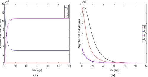
Figure 5. The long-term dynamics of the model system (1(1) $\begin{array}{rl}\frac{\mathrm{d}{S}_u}{\mathrm{d}t}& =\mathrm{\Lambda }-\lambda S_u-\mathrm{d}{S}_u-q{S}_u+\zeta S_q,\\ \frac{\mathrm{d}{S}_q}{\mathrm{d}t}& =q{S}_u+(1-p)\lambda S_u-({ϵ}_q\lambda +\zeta +d)S_q,\\ \frac{\mathrm{d}E}{\mathrm{d}t}& =p\lambda S_u+{ϵ}_q\lambda S_q-(\alpha +d)E,\\ \frac{\mathrm{d}{I}_a}{\mathrm{d}t}& =p_1\alpha E-({\delta }_1+{\varphi }_1+{\gamma }_1+d)I_a,\\ \frac{\mathrm{d}I}{\mathrm{d}t}& =p_2\alpha E-({\delta }_2+{\varphi }_2+{\gamma }_2+d)I,\\ \frac{\mathrm{d}{I}_h}{\mathrm{d}t}& =(1-p_1-p_2)\alpha E+{\varphi }_1{I}_a+{\varphi }_{2}I-({\delta }_3+{\gamma }_3+d)I_h,\\ \frac{\mathrm{d}R}{\mathrm{d}t}& ={\gamma }_1{I}_a+{\gamma }_{2}I+{\gamma }_3{I}_h-\mathrm{d}R,\end{array}$(1) ) when $R_0=0.9529<1.$ The figure ensure the local stability of a EE when $R_0<1$.

4.3. Impact of important parameters on the basic reproduction number $(R_0)$

This section measures how well the basic reproduction number $(R_0)$ evolves in key parameters.

Figure 6. The long-term dynamics of the solutions of model system (1(1) $\begin{array}{rl}\frac{\mathrm{d}{S}_u}{\mathrm{d}t}& =\mathrm{\Lambda }-\lambda S_u-\mathrm{d}{S}_u-q{S}_u+\zeta S_q,\\ \frac{\mathrm{d}{S}_q}{\mathrm{d}t}& =q{S}_u+(1-p)\lambda S_u-({ϵ}_q\lambda +\zeta +d)S_q,\\ \frac{\mathrm{d}E}{\mathrm{d}t}& =p\lambda S_u+{ϵ}_q\lambda S_q-(\alpha +d)E,\\ \frac{\mathrm{d}{I}_a}{\mathrm{d}t}& =p_1\alpha E-({\delta }_1+{\varphi }_1+{\gamma }_1+d)I_a,\\ \frac{\mathrm{d}I}{\mathrm{d}t}& =p_2\alpha E-({\delta }_2+{\varphi }_2+{\gamma }_2+d)I,\\ \frac{\mathrm{d}{I}_h}{\mathrm{d}t}& =(1-p_1-p_2)\alpha E+{\varphi }_1{I}_a+{\varphi }_{2}I-({\delta }_3+{\gamma }_3+d)I_h,\\ \frac{\mathrm{d}R}{\mathrm{d}t}& ={\gamma }_1{I}_a+{\gamma }_{2}I+{\gamma }_3{I}_h-\mathrm{d}R,\end{array}$(1) ) when $R_0=1.3649>1.$ The figure ensure the local stability of a endemic equilibrium when $R_0>1$.

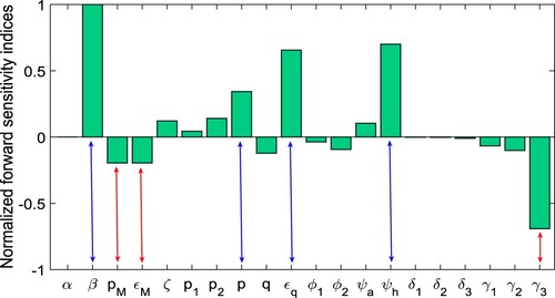
Sensitivity analysis of the basic reproduction number: Using the estimated model parameters (Tables 2 and 4), we perform elasticity analysis to explore the relative significance of all the parameters in the basic reproduction number $R_0$ for COVID-19 in India. Our main goal is to figure out how parametric changes affect the value of $R_0$. The normalized forward sensitivity index of the parameter, Latin hypercube sampling, and partial rank correlation coefficients (PRCC) are used in this investigation. Specifically, the ability to suppress spread of infections is linked to the $R_0$, while disease prevalence is linked to the endemic steady state. By understanding the relative significance of different model parameters in the basic reproduction number, we can identify which control techniques should be used to resist infection spread.

The normalized forward sensitivity index is the ratio of the variable's corresponding difference to the parameter's relative difference. If the variable is a differentiable function of the specified parameter, partial derivatives of the variable with respect to the given parameter can be used to define it. With regard to a parameter $p_i$, the normalized forward sensitivity index of $R_0$ is given by ${\mathrm{\Gamma }}_{p_i}^{R_0}=\frac{\mathrm{\partial }{R}_0}{\mathrm{\partial }{p}_i}\frac{p_i}{R_0}$ An analytical expression for the sensitivity of $R_0$ can be straightforwardly calculated by using the above formula by applying it to each parameter that it includes. For our model (1(1) $\begin{array}{rl}\frac{\mathrm{d}{S}_u}{\mathrm{d}t}& =\mathrm{\Lambda }-\lambda S_u-\mathrm{d}{S}_u-q{S}_u+\zeta S_q,\\ \frac{\mathrm{d}{S}_q}{\mathrm{d}t}& =q{S}_u+(1-p)\lambda S_u-({ϵ}_q\lambda +\zeta +d)S_q,\\ \frac{\mathrm{d}E}{\mathrm{d}t}& =p\lambda S_u+{ϵ}_q\lambda S_q-(\alpha +d)E,\\ \frac{\mathrm{d}{I}_a}{\mathrm{d}t}& =p_1\alpha E-({\delta }_1+{\varphi }_1+{\gamma }_1+d)I_a,\\ \frac{\mathrm{d}I}{\mathrm{d}t}& =p_2\alpha E-({\delta }_2+{\varphi }_2+{\gamma }_2+d)I,\\ \frac{\mathrm{d}{I}_h}{\mathrm{d}t}& =(1-p_1-p_2)\alpha E+{\varphi }_1{I}_a+{\varphi }_{2}I-({\delta }_3+{\gamma }_3+d)I_h,\\ \frac{\mathrm{d}R}{\mathrm{d}t}& ={\gamma }_1{I}_a+{\gamma }_{2}I+{\gamma }_3{I}_h-\mathrm{d}R,\end{array}$(1) ), the normalized forward sensitivity indices of $R_0$ with respect to model parameters are given in Figure 7.

Figure 7. The figure represents the normalized forward sensitivity index for the $R_0$ given in Equation (4(4) $R_0=R_0^I+R_0^{I_a}+R_0^{I_h},$(4) ).

Because of the errors that may occur in identifying, the Latin Hypercube Sampling (LHS) is also shown. A Partial Rank Correlation Coefficient (PRCC) is addressed for the sensitivity analysis between the values of input parameters and those of the basic reproduction number. As a result, the parameters with the greatest PRCC levels do have greatest influence on $R_0$. As a result, the major parameters impacting $R_0$ are divided into those that cause $R_0$ to decline when raised (bars expanding in the lower for negative PRCC levels) and those that allow $R_0$ to grow when increased (bars extending to the upper for positive PRCC values). The PRCC values of the model (1(1) $\begin{array}{rl}\frac{\mathrm{d}{S}_u}{\mathrm{d}t}& =\mathrm{\Lambda }-\lambda S_u-\mathrm{d}{S}_u-q{S}_u+\zeta S_q,\\ \frac{\mathrm{d}{S}_q}{\mathrm{d}t}& =q{S}_u+(1-p)\lambda S_u-({ϵ}_q\lambda +\zeta +d)S_q,\\ \frac{\mathrm{d}E}{\mathrm{d}t}& =p\lambda S_u+{ϵ}_q\lambda S_q-(\alpha +d)E,\\ \frac{\mathrm{d}{I}_a}{\mathrm{d}t}& =p_1\alpha E-({\delta }_1+{\varphi }_1+{\gamma }_1+d)I_a,\\ \frac{\mathrm{d}I}{\mathrm{d}t}& =p_2\alpha E-({\delta }_2+{\varphi }_2+{\gamma }_2+d)I,\\ \frac{\mathrm{d}{I}_h}{\mathrm{d}t}& =(1-p_1-p_2)\alpha E+{\varphi }_1{I}_a+{\varphi }_{2}I-({\delta }_3+{\gamma }_3+d)I_h,\\ \frac{\mathrm{d}R}{\mathrm{d}t}& ={\gamma }_1{I}_a+{\gamma }_{2}I+{\gamma }_3{I}_h-\mathrm{d}R,\end{array}$(1) ) relative to the parameters in $R_0$ are demonstrated in Figure 8 by carrying out 2000 runs of the LHS. In Figure 8, we observe that the most sensitive parameters with high positive PRCC values that control the transmission dynamics of the model are $\beta ,{ϵ}_q$, and ${\psi }_h,$ followed by $p,{\psi }_a,\zeta ,p_2,$ and $p_1.$ Hence, the model parameters $\beta ,{ϵ}_q$, ${\psi }_h,$ $p,{\psi }_a,\zeta ,p_2,$ and $p_1$ are positively correlated with the basic reproduction number. Similarly, the model parameters $p_M,{ϵ}_M$ followed by ${\gamma }_3,q,{\varphi }_1,{\varphi }_2,{\gamma }_1$ and ${\gamma }_2$ have most high negative PRCC values. Thus, the model parameter $p_M,{ϵ}_M$ ${\gamma }_3,q,{\varphi }_1,{\varphi }_2,{\gamma }_1$ are negatively correlated with $R_0$.

Figure 8. The figure depicts the PRCCs for the basic reproduction number $R_0$ given in Equation (4(4) $R_0=R_0^I+R_0^{I_a}+R_0^{I_h},$(4) ).

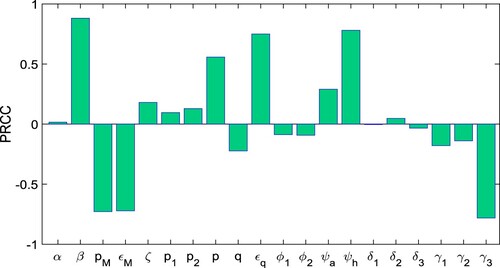
Figure 9. The figure depicts the threshold dynamics of $R_0$ discussed in Section 3.5.

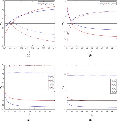
Threshold dynamics of $R_0$: Here, we plot the $R_0$ for the model parameters which are related to various control measures to validate the theoretical findings discussed in Section 3.5. In Figure 9(a), we observe that the rate at which the quarantined susceptible people come back to unquarantined susceptible $(\zeta )$ has a positive impact on the basic reproduction number when $p>{ϵ}_q$ and negative impact to $R_0$ when $p<{ϵ}_q.$ Similarly, in Figure 9(b), the quarantine rate of unquarantined susceptible individuals (q) has a positive influence for the basic reproduction number when $p>{ϵ}_q$. Further, from Figure 9(c), it is clear that isolation of asymptomatic infected individuals is fruitful in controlling the disease when the modification factor of asymptomatic isolated individuals has values less than its threshold value $({\psi }_{h1}^{\ast })$. Thus, if the infectivity of isolated individuals increases to the threshold value $({\psi }_{h1}^{\ast })$ then the isolation of asymptomatic individuals will be harmful to the disease control. Similarly, from Figure 9(d), we have that isolation of symptomatic infected individuals helps to control the disease when infectivity of isolated individuals has the value less than its threshold value $({\psi }_{h2}^{\ast })$. Therefore, from Figures 9(c,d), we conclude that the infectivity of isolated infected individuals should be maintained below its threshold value $({\psi }_h^{\ast }=min\{{\psi }_{h1}^{\ast }{\psi }_{h2}^{\ast }\})$ for the successful isolation program. As a result of the information, it appears that hygienic quarantine and efficient isolation will indeed be adequate protection strategies in India to decrease the COVID-19 incidence.

Surface plots of $R_0$ for various combination of control parameters: The Figures 10(a–d) show the dependence of $R_0$ with respect to $p_M$ (proportion of individuals that wear the face-mask) and ${ϵ}_M$ (efficacy of face masks), ζ (the rate at which the quarantined susceptible go back to unquarantined susceptible class) and q (the rate at which the people goes to quarantine class), ${\psi }_h$ (modification factor for isolated infected individuals), ${\psi }_a$ (modification factor for the asymptomatic infected individuals), ${\varphi }_1$ (isolation rate of asymptomatic infected individuals), and ${\varphi }_2$ (isolation rate of symptomatic infected individuals) for COVID-19 cases in India. In Figure 10(a), we notice that for increasing the values of proportion of individuals that wear the face masks in public ($p_M$) and efficacy of face masks (${ϵ}_M$), the value of the basic reproduction number $R_0$ decreases. In Figure 10(b), we observe that for increasing values of ζ, the value of $R_0$ increases drastically when the model parameter q has a small value. However, the effect of the rate at which quarantined people go back to unquarantined susceptible people ζ will be controlled by increasing value of quarantine rate (q). Therefore, we conclude that in case of a low quarantine rate, if the quarantined people go back to unquarantined susceptible, then it may be harmful to the disease transmission dynamics. In Figure 10(c), we notice that for decreasing the value of infectivity of isolated and asymptomatic infected individuals $({\psi }_h\mathrm{and}{\psi }_a)$, the basic reproduction number $(R_0)$ also decreases to a significant level (below than unity). However, we also observe that the value of $R_0$ is most affected by infectivity of the isolated infected individual. From Figure 10(d), we observe that the isolation rate of asymptomatic and symptomatic infected individuals have the same effect on $R_0$ and by increasing these isolation rates, we can maintain the value of $R_0$ to below unity. Thus, from Figure 10, overall, we believe that in order to reduce COVID-19 transmission, the $R_0$ must be kept below unity with perfect efficacy quarantine, which can be accomplished by maintaining the use of face masks, the infectivity of isolated infected individuals, and infected individual contact tracing.

Since we all know, the magnitude of $R_0$ describes the characteristics of contagious diseases. From Figure 7–10, we see that the improvement in model parameters with negative indices can reduce the value of $R_0$ significantly. The model parameters, namely $\beta ,p,{ϵ}_q,{\psi }_a$, and ${\psi }_h$, have the most positive indices. Thus, the control of the COVID-19 outbreak in India could be achieved by lowering these factors. Furthermore, we discover that these parameters are connected with unquarantined susceptible populations and are also the most relevant parameters based on the sensitivity indices and PRCC values. As a result, we may positively reduce these model parameters. The model parameters $p_M,{ϵ}_M$, and ${\gamma }_3$ have the most negative indices, and these three parameters are also lowering the level of the COVID-19 outbreak in India. As a result, we can determine that the most effective way to keep the COVID-19 disease at lower level is to lower the values of the parameters with positive indices, namely $\beta ,p,{ϵ}_q,{\psi }_a,{\psi }_h$ and to increase the value of the three parameters with negative indices namely $p_M,{ϵ}_M$, and ${\gamma }_3.$ In other words, as the strength of the control strategy improves, the basic reproduction number $R_0$ decreases, and if $R_0$ falls below unity, the infected population will die out.

Figure 10. The figure depicts the impact of important model parameters on the $R_0$ for model system (1(1) $\begin{array}{rl}\frac{\mathrm{d}{S}_u}{\mathrm{d}t}& =\mathrm{\Lambda }-\lambda S_u-\mathrm{d}{S}_u-q{S}_u+\zeta S_q,\\ \frac{\mathrm{d}{S}_q}{\mathrm{d}t}& =q{S}_u+(1-p)\lambda S_u-({ϵ}_q\lambda +\zeta +d)S_q,\\ \frac{\mathrm{d}E}{\mathrm{d}t}& =p\lambda S_u+{ϵ}_q\lambda S_q-(\alpha +d)E,\\ \frac{\mathrm{d}{I}_a}{\mathrm{d}t}& =p_1\alpha E-({\delta }_1+{\varphi }_1+{\gamma }_1+d)I_a,\\ \frac{\mathrm{d}I}{\mathrm{d}t}& =p_2\alpha E-({\delta }_2+{\varphi }_2+{\gamma }_2+d)I,\\ \frac{\mathrm{d}{I}_h}{\mathrm{d}t}& =(1-p_1-p_2)\alpha E+{\varphi }_1{I}_a+{\varphi }_{2}I-({\delta }_3+{\gamma }_3+d)I_h,\\ \frac{\mathrm{d}R}{\mathrm{d}t}& ={\gamma }_1{I}_a+{\gamma }_{2}I+{\gamma }_3{I}_h-\mathrm{d}R,\end{array}$(1) ). The numerical values of all parameter other than (a) $p_M$ and ${ϵ}_M$; (b) ζ and q; (c) ${\psi }_h$ and ${\psi }_a$; (d) ${\varphi }_1$ and ${\varphi }_2$ are given in Tables 2 and 4. (a) Effect of $p_M$ and ${ϵ}_M$ on basic reproduction number $(R_0).$ (b) Effect of ζ and q on basic reproduction number $(R_0).$ (c) Effect of ${\psi }_h$ and ${\psi }_a$ on basic reproduction number $(R_0).$ and (d) Effect of ${\varphi }_1$ and ${\varphi }_2$ on basic reproduction number $(R_0).$

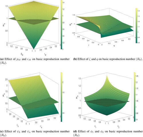
5. Optimal control problem

This section considers an optimal control problem to study the optimal control measures for COVID-19 transmission. Here, we instigate three control functions ${\mu }_1(t),{\mu }_2(t),$ and ${\mu }_3(t)$. The first control ${\mu }_1(t)$ represents preventive measures such as lock-down, social distancing, awareness, etc., that help to reduce the contact between susceptible and infected individuals. The control ${\mu }_2(t)$ represents the testing rate on which hospitalization/isolation of an individual is confirmed, and it helps to reduce the infection risk of susceptible people. The control ${\mu }_3(t)$ involves giving intensive medical care to all diagnosed or hospitalized cases in order to improve the recovery rate. The following system of nonlinear ordinary differential equations provides the controlling mathematical model: (19) $\begin{array}{rl}\frac{\mathrm{d}{S}_u}{\mathrm{d}t}& =\mathrm{\Lambda }-\lambda (1-{\mu }_1(t))S_u-\mathrm{d}{S}_u-q{S}_u+\zeta S_q,\\ \frac{\mathrm{d}{S}_q}{\mathrm{d}t}& =q{S}_u+(1-p)(1-{\mu }_1(t))\lambda S_u-({ϵ}_q\lambda (1-{\mu }_1(t))+\zeta +d)S_q,\\ \frac{\mathrm{d}E}{\mathrm{d}t}& =p\lambda (1-{\mu }_1(t))S_u+{ϵ}_q\lambda (1-{\mu }_1(t))S_q-(\alpha +d)E,\\ \frac{\mathrm{d}{I}_a}{\mathrm{d}t}& =p_1\alpha E-({\delta }_1+{\gamma }_1+d)I_a-{\varphi }_1(1+{\mu }_2(t))I_a,\\ \frac{\mathrm{d}I}{\mathrm{d}t}& =p_2\alpha E-({\delta }_2+{\gamma }_2+d)I-{\varphi }_2(1+{\mu }_2(t))I,\\ \frac{\mathrm{d}{I}_h}{\mathrm{d}t}& =(1-p_1-p_2)\alpha E+{\varphi }_1(1+{\mu }_2(t))I_a\\ & +{\varphi }_2(1+{\mu }_2(t))I-({\delta }_3+{\gamma }_3+d)I_h-{\mu }_3(t)I_h,\\ \frac{\mathrm{d}R}{\mathrm{d}t}& ={\gamma }_1{I}_a+{\gamma }_{2}I+{\gamma }_3{I}_h+{\mu }_3(t)I_h-\mathrm{d}R,\end{array}$(19) where $\lambda =\frac{\beta (1-p_M{ϵ}_M)(I+{\psi }_a{I}_a+{\psi }_h{I}_h)}{N-{ϵ}_h{I}_h}.$ We assume the initial conditions $S_u(0)>0,S_q(0)\ge 0,E(0)\ge 0,I_a(0)\ge 0,I(0)\ge 0,I_h(0)\ge 0,R(0)\ge 0.$ We significantly reduce the total number of COVID-19-exposed, asymptomatic, symptomatic, and hospitalized people using the control variables, ${\mu }_1(t),{\mu }_2(t),$ and ${\mu }_3(t)$ in the model. For this, We also present the positivity of considered control variables ${\mu }_1(t),{\mu }_2(t),$ and ${\mu }_3(t)$ for all time. For this, we define the following objective function [44] $J={\int }_0^T(A_{1}E+A_2{I}_a+A_{3}I+A_4{I}_h+\frac{1}{2}{c}_1{\mu }_1^2++\frac{1}{2}{c}_2{\mu }_2^2++\frac{1}{2}{c}_3{\mu }_3^2)\mathrm{d}t,$ subject to model (19(19) $\begin{array}{rl}\frac{\mathrm{d}{S}_u}{\mathrm{d}t}& =\mathrm{\Lambda }-\lambda (1-{\mu }_1(t))S_u-\mathrm{d}{S}_u-q{S}_u+\zeta S_q,\\ \frac{\mathrm{d}{S}_q}{\mathrm{d}t}& =q{S}_u+(1-p)(1-{\mu }_1(t))\lambda S_u-({ϵ}_q\lambda (1-{\mu }_1(t))+\zeta +d)S_q,\\ \frac{\mathrm{d}E}{\mathrm{d}t}& =p\lambda (1-{\mu }_1(t))S_u+{ϵ}_q\lambda (1-{\mu }_1(t))S_q-(\alpha +d)E,\\ \frac{\mathrm{d}{I}_a}{\mathrm{d}t}& =p_1\alpha E-({\delta }_1+{\gamma }_1+d)I_a-{\varphi }_1(1+{\mu }_2(t))I_a,\\ \frac{\mathrm{d}I}{\mathrm{d}t}& =p_2\alpha E-({\delta }_2+{\gamma }_2+d)I-{\varphi }_2(1+{\mu }_2(t))I,\\ \frac{\mathrm{d}{I}_h}{\mathrm{d}t}& =(1-p_1-p_2)\alpha E+{\varphi }_1(1+{\mu }_2(t))I_a\\ & +{\varphi }_2(1+{\mu }_2(t))I-({\delta }_3+{\gamma }_3+d)I_h-{\mu }_3(t)I_h,\\ \frac{\mathrm{d}R}{\mathrm{d}t}& ={\gamma }_1{I}_a+{\gamma }_{2}I+{\gamma }_3{I}_h+{\mu }_3(t)I_h-\mathrm{d}R,\end{array}$(19) ), where $A_1\ge 0,A_2\ge 0,A_3\ge 0,A_4\ge 0,c_1\ge 0,c_2\ge 0,c_3\ge 0$ and these represent the weight constants of corresponding variables, respectively. While, the quadratic costs $c_1{\mu }_1^2$, $c_2{\mu }_2^2$ and $c_3{\mu }_3^2$, are associated with the controls ${\mu }_1(t),{\mu }_2(t),$ and ${\mu }_3(t),$ respectively. Whereas any global health intervention involves increased costs in order to reach a larger proportion of the population, we usually take a nonlinear cost function, like the quadratic. The constants $A_1,A_2,A_3,A_4,c_1,c_2$ and $c_3$ are used to make balance between the units of measurement of different controls. These constants may also show the relative value of different types of interventions to the broader public. Here, we also consider the quadratic cost following different epidemic controls discussed in [56, 59]. Thus, the total cost (TC) for all controls is is defined as (20) $TC={\int }_0^T\frac{1}{2}(c_1{\mu }_1^2+c_2{\mu }_2^2+c_3{\mu }_3^2)\mathrm{d}t,$(20) where $c_1,c_2,c_3\ge 0$ are the hypothetical unit costs for the implementation of control interventions. The main aim is to attain an optimal control of ${\mu }_1^{\ast }(t),{\mu }_2^{\ast }(t)$ and ${\mu }_3^{\ast }(t)$ such that (21) $J({\mu }_1^{\ast },{\mu }_2^{\ast },{\mu }_3^{\ast })=min\{({\mu }_1,{\mu }_2,{\mu }_3):{\mu }_1,{\mu }_2,{\mu }_3\in \mathrm{\Omega }\},$(21) where Ω is the control set defined as $\mathrm{\Omega }=\{{\mu }_1,{\mu }_2,{\mu }_3:0\le {\mu }_1,{\mu }_2,{\mu }_3\le 1\text{ and measureble}\text{for }t\in [0,T]\}$. The Lagrangian of the control problem (19(19) $\begin{array}{rl}\frac{\mathrm{d}{S}_u}{\mathrm{d}t}& =\mathrm{\Lambda }-\lambda (1-{\mu }_1(t))S_u-\mathrm{d}{S}_u-q{S}_u+\zeta S_q,\\ \frac{\mathrm{d}{S}_q}{\mathrm{d}t}& =q{S}_u+(1-p)(1-{\mu }_1(t))\lambda S_u-({ϵ}_q\lambda (1-{\mu }_1(t))+\zeta +d)S_q,\\ \frac{\mathrm{d}E}{\mathrm{d}t}& =p\lambda (1-{\mu }_1(t))S_u+{ϵ}_q\lambda (1-{\mu }_1(t))S_q-(\alpha +d)E,\\ \frac{\mathrm{d}{I}_a}{\mathrm{d}t}& =p_1\alpha E-({\delta }_1+{\gamma }_1+d)I_a-{\varphi }_1(1+{\mu }_2(t))I_a,\\ \frac{\mathrm{d}I}{\mathrm{d}t}& =p_2\alpha E-({\delta }_2+{\gamma }_2+d)I-{\varphi }_2(1+{\mu }_2(t))I,\\ \frac{\mathrm{d}{I}_h}{\mathrm{d}t}& =(1-p_1-p_2)\alpha E+{\varphi }_1(1+{\mu }_2(t))I_a\\ & +{\varphi }_2(1+{\mu }_2(t))I-({\delta }_3+{\gamma }_3+d)I_h-{\mu }_3(t)I_h,\\ \frac{\mathrm{d}R}{\mathrm{d}t}& ={\gamma }_1{I}_a+{\gamma }_{2}I+{\gamma }_3{I}_h+{\mu }_3(t)I_h-\mathrm{d}R,\end{array}$(19) ) is defined as $L=A_{1}E+A_2{I}_a+A_{3}I+A_4{I}_h+\frac{1}{2}{c}_1{\mu }_1^2++\frac{1}{2}{c}_2{\mu }_2^2++\frac{1}{2}{c}_3{\mu }_3^2.$ This would have been used to determine the Lagrangian's minimal value. It could be done by specifying an appropriate Hamiltonian. As a result, for our control problem, we constructed Hamiltonian H as follows: (22) $H=L+{\lambda }_1\frac{\mathrm{d}{S}_u}{\mathrm{d}t}+{\lambda }_2\frac{\mathrm{d}{S}_q}{\mathrm{d}t}+{\lambda }_3\frac{\mathrm{d}E}{\mathrm{d}t}+{\lambda }_4\frac{\mathrm{d}{I}_a}{\mathrm{d}t}+{\lambda }_5\frac{\mathrm{d}I}{\mathrm{d}t}+{\lambda }_6\frac{\mathrm{d}{I}_h}{\mathrm{d}t}+{\lambda }_7\frac{\mathrm{d}R}{\mathrm{d}t},$(22) where ${\lambda }_i,i=1,2,\dots 7$ are the adjoint variables and can be obtained by the solving of the following system of differential equations: (23) $\begin{array}{rl}\frac{\mathrm{d}{\lambda }_1}{\mathrm{d}t}=-\frac{\mathrm{\partial }H}{\mathrm{\partial }{S}_u}& ={\lambda }_{1}d+({\lambda }_1-{\lambda }_2)q+({\lambda }_1-{\lambda }_2)\lambda (1-{\mu }_1)+({\lambda }_2-{\lambda }_3)p\lambda (1-{\mu }_1)\\ & +({\lambda }_3+{\lambda }_2-{\lambda }_1)\vartheta (1-{\mu }_1)S_u,\\ \frac{\mathrm{d}{\lambda }_2}{\mathrm{d}t}=-\frac{\mathrm{\partial }H}{\mathrm{\partial }{S}_q}& =({\lambda }_1+{\lambda }_2)\vartheta (1-{\mu }_1)S_u+({\lambda }_3-{\lambda }_2)p\vartheta (1-{\mu }_1)S_u+{\lambda }_1(\zeta +d)\\ & +({\lambda }_2-{\lambda }_3)\lambda (1-{\mu }_1){ϵ}_q+({\lambda }_3-{\lambda }_2){ϵ}_q(1-{\mu }_1)S_q\vartheta ,\\ \frac{\mathrm{d}{\lambda }_3}{\mathrm{d}t}=-\frac{\mathrm{\partial }H}{\mathrm{\partial }E}& =-A_1+({\lambda }_1-{\lambda }_2)\vartheta (1-{\mu }_1)S_u+({\lambda }_2-{\lambda }_3)p\vartheta (1-{\mu }_1)S_q\\ & +({\lambda }_2-{\lambda }_3){ϵ}_q\vartheta (1-{\mu }_1)S_q+{\lambda }_{3}d+({\lambda }_3-{\lambda }_6)\alpha \\ & +({\lambda }_6-{\lambda }_4)p_1\alpha +({\lambda }_6-{\lambda }_5)p_2\alpha ,\\ \frac{\mathrm{d}{\lambda }_4}{\mathrm{d}t}=-\frac{\mathrm{\partial }H}{\mathrm{\partial }{I}_a}& =-A_2+({\lambda }_1-{\lambda }_2)\kappa (1-{\mu }_1){\psi }_a{S}_u+({\lambda }_2-{\lambda }_3)\kappa (1-{\mu }_1){\psi }_a{S}_u\\ & +({\lambda }_2-{\lambda }_1)\vartheta (1-{\mu }_1)S_u+({\lambda }_3-{\lambda }_2)\vartheta (1-{\mu }_1)S_u\\ & +({\lambda }_2-{\lambda }_3){ϵ}_q\kappa (1-{\mu }_1){\psi }_a{S}_q\\ & +({\lambda }_3-{\lambda }_2){ϵ}_q\vartheta (1-{\mu }_1)S_q+({\lambda }_4-{\lambda }_6){\varphi }_1(1+{\mu }_2)\\ & +({\lambda }_4-{\lambda }_7){\gamma }_1+{\lambda }_4({\delta }_1+d),\\ \frac{\mathrm{d}{\lambda }_5}{\mathrm{d}t}=-\frac{\mathrm{\partial }H}{\mathrm{\partial }I}& =-A_3+({\lambda }_1-{\lambda }_2)\kappa (1-{\mu }_1)S_u+({\lambda }_2-{\lambda }_3)p\kappa (1-{\mu }_1)S_u\\ & +({\lambda }_2-{\lambda }_1)\vartheta (1-{\mu }_1)S_u\\ & +({\lambda }_3-{\lambda }_2)\vartheta (1-{\mu }_1)S_u+({\lambda }_2-{\lambda }_3){ϵ}_q\kappa (1-{\mu }_1)S_q\\ & +({\lambda }_3-{\lambda }_2){ϵ}_q\vartheta (1-{\mu }_1)S_q\\ & +({\lambda }_5-{\lambda }_6){\varphi }_2(1+{\mu }_2)+({\lambda }_5-{\lambda }_7){\gamma }_2+{\lambda }_5({\delta }_2+d),\\ \frac{\mathrm{d}{\lambda }_6}{\mathrm{d}t}=-\frac{\mathrm{\partial }H}{\mathrm{\partial }{I}_h}& =-A_4+({\lambda }_1-{\lambda }_2)\kappa (1-{\mu }_1){\psi }_h{S}_u+({\lambda }_2-{\lambda }_3)p\kappa (1-{\mu }_1){\psi }_h{S}_u\\ & +({\lambda }_2-{\lambda }_1)\vartheta (1-{\mu }_1)(1-{ϵ}_h)S_u+({\lambda }_3-{\lambda }_2)p\vartheta (1-{\mu }_1)(1-{ϵ}_h)S_u\\ & +({\lambda }_2-{\lambda }_3){ϵ}_q\kappa (1-{\mu }_1){\psi }_h{S}_q+({\lambda }_3-{\lambda }_2){ϵ}_q\vartheta (1-{\mu }_1)(1-{ϵ}_h)S_q\\ & +({\lambda }_6-{\lambda }_7)({\gamma }_3+{\mu }_3)+{\lambda }_6({\delta }_3+d),\\ \frac{\mathrm{d}{\lambda }_7}{\mathrm{d}t}=-\frac{\mathrm{\partial }H}{\mathrm{\partial }R}& =({\lambda }_1-{\lambda }_2)\vartheta (1-{\mu }_1)S_u+({\lambda }_2-{\lambda }_3)p\vartheta (1-{\mu }_1)S_u\\ & +({\lambda }_2-{\lambda }_3){ϵ}_q\vartheta (1-{\mu }_1)S_q,\end{array}$(23) where $\vartheta =\frac{\lambda }{N-{ϵ}_h{I}_h}\mathrm{and}\kappa =\frac{\beta (1-p_M{ϵ}_M)}{N-{ϵ}_h{I}_h}$ satisfy the transversality condition ${\lambda }_i(T)=0$ for $i=1,2,\dots ,7.$ Let $\widetilde{S_u},\widetilde{S_q},\widetilde{I_a},\tilde{I},\widetilde{I_h},\tilde{R}$ be the optimum values of $S_u,S_q,I_a,I,I_h,R$ and let $\widetilde{{\lambda }_i}$ for $i=1,2,\dots ,7$ are the solution of the system (23(23) $\begin{array}{rl}\frac{\mathrm{d}{\lambda }_1}{\mathrm{d}t}=-\frac{\mathrm{\partial }H}{\mathrm{\partial }{S}_u}& ={\lambda }_{1}d+({\lambda }_1-{\lambda }_2)q+({\lambda }_1-{\lambda }_2)\lambda (1-{\mu }_1)+({\lambda }_2-{\lambda }_3)p\lambda (1-{\mu }_1)\\ & +({\lambda }_3+{\lambda }_2-{\lambda }_1)\vartheta (1-{\mu }_1)S_u,\\ \frac{\mathrm{d}{\lambda }_2}{\mathrm{d}t}=-\frac{\mathrm{\partial }H}{\mathrm{\partial }{S}_q}& =({\lambda }_1+{\lambda }_2)\vartheta (1-{\mu }_1)S_u+({\lambda }_3-{\lambda }_2)p\vartheta (1-{\mu }_1)S_u+{\lambda }_1(\zeta +d)\\ & +({\lambda }_2-{\lambda }_3)\lambda (1-{\mu }_1){ϵ}_q+({\lambda }_3-{\lambda }_2){ϵ}_q(1-{\mu }_1)S_q\vartheta ,\\ \frac{\mathrm{d}{\lambda }_3}{\mathrm{d}t}=-\frac{\mathrm{\partial }H}{\mathrm{\partial }E}& =-A_1+({\lambda }_1-{\lambda }_2)\vartheta (1-{\mu }_1)S_u+({\lambda }_2-{\lambda }_3)p\vartheta (1-{\mu }_1)S_q\\ & +({\lambda }_2-{\lambda }_3){ϵ}_q\vartheta (1-{\mu }_1)S_q+{\lambda }_{3}d+({\lambda }_3-{\lambda }_6)\alpha \\ & +({\lambda }_6-{\lambda }_4)p_1\alpha +({\lambda }_6-{\lambda }_5)p_2\alpha ,\\ \frac{\mathrm{d}{\lambda }_4}{\mathrm{d}t}=-\frac{\mathrm{\partial }H}{\mathrm{\partial }{I}_a}& =-A_2+({\lambda }_1-{\lambda }_2)\kappa (1-{\mu }_1){\psi }_a{S}_u+({\lambda }_2-{\lambda }_3)\kappa (1-{\mu }_1){\psi }_a{S}_u\\ & +({\lambda }_2-{\lambda }_1)\vartheta (1-{\mu }_1)S_u+({\lambda }_3-{\lambda }_2)\vartheta (1-{\mu }_1)S_u\\ & +({\lambda }_2-{\lambda }_3){ϵ}_q\kappa (1-{\mu }_1){\psi }_a{S}_q\\ & +({\lambda }_3-{\lambda }_2){ϵ}_q\vartheta (1-{\mu }_1)S_q+({\lambda }_4-{\lambda }_6){\varphi }_1(1+{\mu }_2)\\ & +({\lambda }_4-{\lambda }_7){\gamma }_1+{\lambda }_4({\delta }_1+d),\\ \frac{\mathrm{d}{\lambda }_5}{\mathrm{d}t}=-\frac{\mathrm{\partial }H}{\mathrm{\partial }I}& =-A_3+({\lambda }_1-{\lambda }_2)\kappa (1-{\mu }_1)S_u+({\lambda }_2-{\lambda }_3)p\kappa (1-{\mu }_1)S_u\\ & +({\lambda }_2-{\lambda }_1)\vartheta (1-{\mu }_1)S_u\\ & +({\lambda }_3-{\lambda }_2)\vartheta (1-{\mu }_1)S_u+({\lambda }_2-{\lambda }_3){ϵ}_q\kappa (1-{\mu }_1)S_q\\ & +({\lambda }_3-{\lambda }_2){ϵ}_q\vartheta (1-{\mu }_1)S_q\\ & +({\lambda }_5-{\lambda }_6){\varphi }_2(1+{\mu }_2)+({\lambda }_5-{\lambda }_7){\gamma }_2+{\lambda }_5({\delta }_2+d),\\ \frac{\mathrm{d}{\lambda }_6}{\mathrm{d}t}=-\frac{\mathrm{\partial }H}{\mathrm{\partial }{I}_h}& =-A_4+({\lambda }_1-{\lambda }_2)\kappa (1-{\mu }_1){\psi }_h{S}_u+({\lambda }_2-{\lambda }_3)p\kappa (1-{\mu }_1){\psi }_h{S}_u\\ & +({\lambda }_2-{\lambda }_1)\vartheta (1-{\mu }_1)(1-{ϵ}_h)S_u+({\lambda }_3-{\lambda }_2)p\vartheta (1-{\mu }_1)(1-{ϵ}_h)S_u\\ & +({\lambda }_2-{\lambda }_3){ϵ}_q\kappa (1-{\mu }_1){\psi }_h{S}_q+({\lambda }_3-{\lambda }_2){ϵ}_q\vartheta (1-{\mu }_1)(1-{ϵ}_h)S_q\\ & +({\lambda }_6-{\lambda }_7)({\gamma }_3+{\mu }_3)+{\lambda }_6({\delta }_3+d),\\ \frac{\mathrm{d}{\lambda }_7}{\mathrm{d}t}=-\frac{\mathrm{\partial }H}{\mathrm{\partial }R}& =({\lambda }_1-{\lambda }_2)\vartheta (1-{\mu }_1)S_u+({\lambda }_2-{\lambda }_3)p\vartheta (1-{\mu }_1)S_u\\ & +({\lambda }_2-{\lambda }_3){ϵ}_q\vartheta (1-{\mu }_1)S_q,\end{array}$(23) ). By using some results discussed in [57], we establish the Theorem 5.1.

Theorem 5.1

There exist optimal controls ${\mu }_1^{\ast },{\mu }_2^{\ast },{\mu }_3^{\ast }\in \mathrm{\Omega }$ such that $J({\mu }_1^{\ast },{\mu }_2^{\ast },{\mu }_3^{\ast })=\underset{{\mu }_1,{\mu }_2,{\mu }_3\in \mathrm{\Omega }}{min}J({\mu }_1,{\mu }_2,{\mu }_3)$ subject to system (19(19) $\begin{array}{rl}\frac{\mathrm{d}{S}_u}{\mathrm{d}t}& =\mathrm{\Lambda }-\lambda (1-{\mu }_1(t))S_u-\mathrm{d}{S}_u-q{S}_u+\zeta S_q,\\ \frac{\mathrm{d}{S}_q}{\mathrm{d}t}& =q{S}_u+(1-p)(1-{\mu }_1(t))\lambda S_u-({ϵ}_q\lambda (1-{\mu }_1(t))+\zeta +d)S_q,\\ \frac{\mathrm{d}E}{\mathrm{d}t}& =p\lambda (1-{\mu }_1(t))S_u+{ϵ}_q\lambda (1-{\mu }_1(t))S_q-(\alpha +d)E,\\ \frac{\mathrm{d}{I}_a}{\mathrm{d}t}& =p_1\alpha E-({\delta }_1+{\gamma }_1+d)I_a-{\varphi }_1(1+{\mu }_2(t))I_a,\\ \frac{\mathrm{d}I}{\mathrm{d}t}& =p_2\alpha E-({\delta }_2+{\gamma }_2+d)I-{\varphi }_2(1+{\mu }_2(t))I,\\ \frac{\mathrm{d}{I}_h}{\mathrm{d}t}& =(1-p_1-p_2)\alpha E+{\varphi }_1(1+{\mu }_2(t))I_a\\ & +{\varphi }_2(1+{\mu }_2(t))I-({\delta }_3+{\gamma }_3+d)I_h-{\mu }_3(t)I_h,\\ \frac{\mathrm{d}R}{\mathrm{d}t}& ={\gamma }_1{I}_a+{\gamma }_{2}I+{\gamma }_3{I}_h+{\mu }_3(t)I_h-\mathrm{d}R,\end{array}$(19) ).

Proof.

Since the state variables and controls are positive in system (19(19) $\begin{array}{rl}\frac{\mathrm{d}{S}_u}{\mathrm{d}t}& =\mathrm{\Lambda }-\lambda (1-{\mu }_1(t))S_u-\mathrm{d}{S}_u-q{S}_u+\zeta S_q,\\ \frac{\mathrm{d}{S}_q}{\mathrm{d}t}& =q{S}_u+(1-p)(1-{\mu }_1(t))\lambda S_u-({ϵ}_q\lambda (1-{\mu }_1(t))+\zeta +d)S_q,\\ \frac{\mathrm{d}E}{\mathrm{d}t}& =p\lambda (1-{\mu }_1(t))S_u+{ϵ}_q\lambda (1-{\mu }_1(t))S_q-(\alpha +d)E,\\ \frac{\mathrm{d}{I}_a}{\mathrm{d}t}& =p_1\alpha E-({\delta }_1+{\gamma }_1+d)I_a-{\varphi }_1(1+{\mu }_2(t))I_a,\\ \frac{\mathrm{d}I}{\mathrm{d}t}& =p_2\alpha E-({\delta }_2+{\gamma }_2+d)I-{\varphi }_2(1+{\mu }_2(t))I,\\ \frac{\mathrm{d}{I}_h}{\mathrm{d}t}& =(1-p_1-p_2)\alpha E+{\varphi }_1(1+{\mu }_2(t))I_a\\ & +{\varphi }_2(1+{\mu }_2(t))I-({\delta }_3+{\gamma }_3+d)I_h-{\mu }_3(t)I_h,\\ \frac{\mathrm{d}R}{\mathrm{d}t}& ={\gamma }_1{I}_a+{\gamma }_{2}I+{\gamma }_3{I}_h+{\mu }_3(t)I_h-\mathrm{d}R,\end{array}$(19) ). For the minimization problem, the convexity of the objective functional in $({\mu }_1,{\mu }_2,{\mu }_3)$ should be satisfied [57]. Here, we have that the control variable set Ω, where ${\mu }_1,{\mu }_2,{\mu }_3\in \mathrm{\Omega }$ is convex and closed by definition. The integrand of functional $A_{1}E+A_2{I}_a+A_{3}I+A_4{I}_h+\frac{1}{2}{c}_1{\mu }_1^2++\frac{1}{2}{c}_2{\mu }_2^2++\frac{1}{2}{c}_3{\mu }_3^2$ is also convex on the control variable set Ω and the state variables are also bounded. Since there occurs an optimal control for minimizing the functional subject to the given mathematical model and adjoint variables, therefore, we use Pontryagin's maximum principle to derive required conditions and to obtain an optimal solution for the control problem (19(19) $\begin{array}{rl}\frac{\mathrm{d}{S}_u}{\mathrm{d}t}& =\mathrm{\Lambda }-\lambda (1-{\mu }_1(t))S_u-\mathrm{d}{S}_u-q{S}_u+\zeta S_q,\\ \frac{\mathrm{d}{S}_q}{\mathrm{d}t}& =q{S}_u+(1-p)(1-{\mu }_1(t))\lambda S_u-({ϵ}_q\lambda (1-{\mu }_1(t))+\zeta +d)S_q,\\ \frac{\mathrm{d}E}{\mathrm{d}t}& =p\lambda (1-{\mu }_1(t))S_u+{ϵ}_q\lambda (1-{\mu }_1(t))S_q-(\alpha +d)E,\\ \frac{\mathrm{d}{I}_a}{\mathrm{d}t}& =p_1\alpha E-({\delta }_1+{\gamma }_1+d)I_a-{\varphi }_1(1+{\mu }_2(t))I_a,\\ \frac{\mathrm{d}I}{\mathrm{d}t}& =p_2\alpha E-({\delta }_2+{\gamma }_2+d)I-{\varphi }_2(1+{\mu }_2(t))I,\\ \frac{\mathrm{d}{I}_h}{\mathrm{d}t}& =(1-p_1-p_2)\alpha E+{\varphi }_1(1+{\mu }_2(t))I_a\\ & +{\varphi }_2(1+{\mu }_2(t))I-({\delta }_3+{\gamma }_3+d)I_h-{\mu }_3(t)I_h,\\ \frac{\mathrm{d}R}{\mathrm{d}t}& ={\gamma }_1{I}_a+{\gamma }_{2}I+{\gamma }_3{I}_h+{\mu }_3(t)I_h-\mathrm{d}R,\end{array}$(19) ).

According to [56, 59], if $(x,\mu )$ is an optimal solution of an optimal control problem then there exists a non-trivial vector function $\mathrm{\Gamma }=({\mu }_1,{\mu }_2,{\mu }_3)$ satisfying the following equalities: (24) $\frac{\mathrm{d}x}{\mathrm{d}t}=\frac{\mathrm{\partial }H(t,x,\mu ,\mathrm{\Gamma })}{\mathrm{\partial }\mathrm{\Gamma }},0=\frac{\mathrm{\partial }H(t,x,\mu ,\mathrm{\Gamma })}{\mathrm{\partial }\mathrm{\Gamma }},\frac{\mathrm{d}\mathrm{\Gamma }}{\mathrm{d}t}=\frac{\mathrm{\partial }H(t,x,\mu ,\mathrm{\Gamma })}{\mathrm{\partial }\mathrm{\Gamma }}.$(24) To compute the optimal control of the control variable set, where $0\le {\mu }_i\le 1$ for $i=1,2,3,$ let $S_u=\widetilde{S_u},S_q=\widetilde{S_q},I_a=\widetilde{I_a},I=\tilde{I},I_h=\widetilde{I_h},R=\tilde{R}.$ By differentiating Hamiltonian H of Equation (22(22) $H=L+{\lambda }_1\frac{\mathrm{d}{S}_u}{\mathrm{d}t}+{\lambda }_2\frac{\mathrm{d}{S}_q}{\mathrm{d}t}+{\lambda }_3\frac{\mathrm{d}E}{\mathrm{d}t}+{\lambda }_4\frac{\mathrm{d}{I}_a}{\mathrm{d}t}+{\lambda }_5\frac{\mathrm{d}I}{\mathrm{d}t}+{\lambda }_6\frac{\mathrm{d}{I}_h}{\mathrm{d}t}+{\lambda }_7\frac{\mathrm{d}R}{\mathrm{d}t},$(22) ) with respect to control variables ${\mu }_1,{\mu }_2$ and ${\mu }_3$, we obtain (25) $\begin{array}{rl}\frac{\mathrm{\partial }H}{\mathrm{\partial }{\mu }_1}& =c_1{\mu }_1-({\lambda }_2-{\lambda }_1)\lambda \widetilde{S_u}-({\lambda }_3-{\lambda }_2)p\lambda \widetilde{S_u}-({\lambda }_3-{\lambda }_2){ϵ}_q\lambda \widetilde{S_q},\\ \frac{\mathrm{\partial }H}{\mathrm{\partial }{\mu }_2}& =c_1{\mu }_2-({\lambda }_4-{\lambda }_6){\varphi }_1\widetilde{I_a}-({\lambda }_5-{\lambda }_6){\varphi }_2\tilde{I},\\ \frac{\mathrm{\partial }H}{\mathrm{\partial }{\mu }_3}& =c_1{\mu }_3-({\lambda }_6-{\lambda }_7)\widetilde{I_h}.\end{array}$(25) We apply the second condition of Equation (24(24) $\frac{\mathrm{d}x}{\mathrm{d}t}=\frac{\mathrm{\partial }H(t,x,\mu ,\mathrm{\Gamma })}{\mathrm{\partial }\mathrm{\Gamma }},0=\frac{\mathrm{\partial }H(t,x,\mu ,\mathrm{\Gamma })}{\mathrm{\partial }\mathrm{\Gamma }},\frac{\mathrm{d}\mathrm{\Gamma }}{\mathrm{d}t}=\frac{\mathrm{\partial }H(t,x,\mu ,\mathrm{\Gamma })}{\mathrm{\partial }\mathrm{\Gamma }}.$(24) ) (optimality condition) $\frac{\mathrm{\partial }H}{\mathrm{\partial }{\mu }_1}=0,\frac{\mathrm{\partial }H}{\mathrm{\partial }{\mu }_2}=0,\frac{\mathrm{\partial }H}{\mathrm{\partial }{\mu }_3}=0,$ and solve Equation (25(25) $\begin{array}{rl}\frac{\mathrm{\partial }H}{\mathrm{\partial }{\mu }_1}& =c_1{\mu }_1-({\lambda }_2-{\lambda }_1)\lambda \widetilde{S_u}-({\lambda }_3-{\lambda }_2)p\lambda \widetilde{S_u}-({\lambda }_3-{\lambda }_2){ϵ}_q\lambda \widetilde{S_q},\\ \frac{\mathrm{\partial }H}{\mathrm{\partial }{\mu }_2}& =c_1{\mu }_2-({\lambda }_4-{\lambda }_6){\varphi }_1\widetilde{I_a}-({\lambda }_5-{\lambda }_6){\varphi }_2\tilde{I},\\ \frac{\mathrm{\partial }H}{\mathrm{\partial }{\mu }_3}& =c_1{\mu }_3-({\lambda }_6-{\lambda }_7)\widetilde{I_h}.\end{array}$(25) ), we have $\begin{array}{rl}{\mu }_1& =\frac{({\lambda }_3-{\lambda }_2)\lambda (p{S}_u+{ϵ}_q{S}_q)+({\lambda }_2-{\lambda }_1)\lambda S_u}{c_1}=\widetilde{{\mu }_1},\\ {\mu }_2& =\frac{({\lambda }_4-{\lambda }_6){\varphi }_1{I}_a+({\lambda }_5-{\lambda }_6){\varphi }_{2}I}{c_2}=\widetilde{{\mu }_2},{\mu }_3=\frac{({\lambda }_6-{\lambda }_7)I_h}{c_3}=\widetilde{{\mu }_3}.\end{array}$ The upper and lower bounds for these controls are 0 and ${\mu }_1^{max}$, ${\mu }_2^{max}$, ${\mu }_3^{max},$ respectively, i.e. ${\mu }_1={\mu }_2={\mu }_3=0$ if $\widetilde{{\mu }_1}<0,\widetilde{{\mu }_2}<0,$ and $\widetilde{{\mu }_3}<0.$ These controls attain its maximum i.e. ${\mu }_1={\mu }_1^{max},{\mu }_2={\mu }_2^{max},$ and ${\mu }_3={\mu }_3^{max}$ if $\widetilde{{\mu }_1}>{\mu }_1^{max},\widetilde{{\mu }_2}>{\mu }_2^{max},$ and $\widetilde{{\mu }_3}>{\mu }_3^{max}$, otherwise ${\mu }_1=\widetilde{{\mu }_1},{\mu }_2=\widetilde{{\mu }_2}$ and ${\mu }_3=\widetilde{{\mu }_3}.$ Hence, for these optimal controls ${\mu }_1^{\ast }$, ${\mu }_2^{\ast }$, ${\mu }_3^{\ast }$, we attain the optimum value of the function J and optimal controls are given as follows: $\begin{array}{rl}{\mu }_1^{\ast }& =min\{{\mu }_1^{max},max\{0,\widetilde{{\mu }_1}\}\},{\mu }_2^{\ast }=min\{{\mu }_2^{max},max\{0,\widetilde{{\mu }_2}\}\},\\ {\mu }_3^{\ast }& =min\{{\mu }_3^{max},max\{0,\widetilde{{\mu }_3}\}\}.\text{■}\end{array}$

5.1. Numerical results of the optimal control analysis

The forward-backward sweep (implemented in MATLAB) is used to solve the optimality system comprising the state Equation (19(19) $\begin{array}{rl}\frac{\mathrm{d}{S}_u}{\mathrm{d}t}& =\mathrm{\Lambda }-\lambda (1-{\mu }_1(t))S_u-\mathrm{d}{S}_u-q{S}_u+\zeta S_q,\\ \frac{\mathrm{d}{S}_q}{\mathrm{d}t}& =q{S}_u+(1-p)(1-{\mu }_1(t))\lambda S_u-({ϵ}_q\lambda (1-{\mu }_1(t))+\zeta +d)S_q,\\ \frac{\mathrm{d}E}{\mathrm{d}t}& =p\lambda (1-{\mu }_1(t))S_u+{ϵ}_q\lambda (1-{\mu }_1(t))S_q-(\alpha +d)E,\\ \frac{\mathrm{d}{I}_a}{\mathrm{d}t}& =p_1\alpha E-({\delta }_1+{\gamma }_1+d)I_a-{\varphi }_1(1+{\mu }_2(t))I_a,\\ \frac{\mathrm{d}I}{\mathrm{d}t}& =p_2\alpha E-({\delta }_2+{\gamma }_2+d)I-{\varphi }_2(1+{\mu }_2(t))I,\\ \frac{\mathrm{d}{I}_h}{\mathrm{d}t}& =(1-p_1-p_2)\alpha E+{\varphi }_1(1+{\mu }_2(t))I_a\\ & +{\varphi }_2(1+{\mu }_2(t))I-({\delta }_3+{\gamma }_3+d)I_h-{\mu }_3(t)I_h,\\ \frac{\mathrm{d}R}{\mathrm{d}t}& ={\gamma }_1{I}_a+{\gamma }_{2}I+{\gamma }_3{I}_h+{\mu }_3(t)I_h-\mathrm{d}R,\end{array}$(19) ) and adjoint Equation (23(23) $\begin{array}{rl}\frac{\mathrm{d}{\lambda }_1}{\mathrm{d}t}=-\frac{\mathrm{\partial }H}{\mathrm{\partial }{S}_u}& ={\lambda }_{1}d+({\lambda }_1-{\lambda }_2)q+({\lambda }_1-{\lambda }_2)\lambda (1-{\mu }_1)+({\lambda }_2-{\lambda }_3)p\lambda (1-{\mu }_1)\\ & +({\lambda }_3+{\lambda }_2-{\lambda }_1)\vartheta (1-{\mu }_1)S_u,\\ \frac{\mathrm{d}{\lambda }_2}{\mathrm{d}t}=-\frac{\mathrm{\partial }H}{\mathrm{\partial }{S}_q}& =({\lambda }_1+{\lambda }_2)\vartheta (1-{\mu }_1)S_u+({\lambda }_3-{\lambda }_2)p\vartheta (1-{\mu }_1)S_u+{\lambda }_1(\zeta +d)\\ & +({\lambda }_2-{\lambda }_3)\lambda (1-{\mu }_1){ϵ}_q+({\lambda }_3-{\lambda }_2){ϵ}_q(1-{\mu }_1)S_q\vartheta ,\\ \frac{\mathrm{d}{\lambda }_3}{\mathrm{d}t}=-\frac{\mathrm{\partial }H}{\mathrm{\partial }E}& =-A_1+({\lambda }_1-{\lambda }_2)\vartheta (1-{\mu }_1)S_u+({\lambda }_2-{\lambda }_3)p\vartheta (1-{\mu }_1)S_q\\ & +({\lambda }_2-{\lambda }_3){ϵ}_q\vartheta (1-{\mu }_1)S_q+{\lambda }_{3}d+({\lambda }_3-{\lambda }_6)\alpha \\ & +({\lambda }_6-{\lambda }_4)p_1\alpha +({\lambda }_6-{\lambda }_5)p_2\alpha ,\\ \frac{\mathrm{d}{\lambda }_4}{\mathrm{d}t}=-\frac{\mathrm{\partial }H}{\mathrm{\partial }{I}_a}& =-A_2+({\lambda }_1-{\lambda }_2)\kappa (1-{\mu }_1){\psi }_a{S}_u+({\lambda }_2-{\lambda }_3)\kappa (1-{\mu }_1){\psi }_a{S}_u\\ & +({\lambda }_2-{\lambda }_1)\vartheta (1-{\mu }_1)S_u+({\lambda }_3-{\lambda }_2)\vartheta (1-{\mu }_1)S_u\\ & +({\lambda }_2-{\lambda }_3){ϵ}_q\kappa (1-{\mu }_1){\psi }_a{S}_q\\ & +({\lambda }_3-{\lambda }_2){ϵ}_q\vartheta (1-{\mu }_1)S_q+({\lambda }_4-{\lambda }_6){\varphi }_1(1+{\mu }_2)\\ & +({\lambda }_4-{\lambda }_7){\gamma }_1+{\lambda }_4({\delta }_1+d),\\ \frac{\mathrm{d}{\lambda }_5}{\mathrm{d}t}=-\frac{\mathrm{\partial }H}{\mathrm{\partial }I}& =-A_3+({\lambda }_1-{\lambda }_2)\kappa (1-{\mu }_1)S_u+({\lambda }_2-{\lambda }_3)p\kappa (1-{\mu }_1)S_u\\ & +({\lambda }_2-{\lambda }_1)\vartheta (1-{\mu }_1)S_u\\ & +({\lambda }_3-{\lambda }_2)\vartheta (1-{\mu }_1)S_u+({\lambda }_2-{\lambda }_3){ϵ}_q\kappa (1-{\mu }_1)S_q\\ & +({\lambda }_3-{\lambda }_2){ϵ}_q\vartheta (1-{\mu }_1)S_q\\ & +({\lambda }_5-{\lambda }_6){\varphi }_2(1+{\mu }_2)+({\lambda }_5-{\lambda }_7){\gamma }_2+{\lambda }_5({\delta }_2+d),\\ \frac{\mathrm{d}{\lambda }_6}{\mathrm{d}t}=-\frac{\mathrm{\partial }H}{\mathrm{\partial }{I}_h}& =-A_4+({\lambda }_1-{\lambda }_2)\kappa (1-{\mu }_1){\psi }_h{S}_u+({\lambda }_2-{\lambda }_3)p\kappa (1-{\mu }_1){\psi }_h{S}_u\\ & +({\lambda }_2-{\lambda }_1)\vartheta (1-{\mu }_1)(1-{ϵ}_h)S_u+({\lambda }_3-{\lambda }_2)p\vartheta (1-{\mu }_1)(1-{ϵ}_h)S_u\\ & +({\lambda }_2-{\lambda }_3){ϵ}_q\kappa (1-{\mu }_1){\psi }_h{S}_q+({\lambda }_3-{\lambda }_2){ϵ}_q\vartheta (1-{\mu }_1)(1-{ϵ}_h)S_q\\ & +({\lambda }_6-{\lambda }_7)({\gamma }_3+{\mu }_3)+{\lambda }_6({\delta }_3+d),\\ \frac{\mathrm{d}{\lambda }_7}{\mathrm{d}t}=-\frac{\mathrm{\partial }H}{\mathrm{\partial }R}& =({\lambda }_1-{\lambda }_2)\vartheta (1-{\mu }_1)S_u+({\lambda }_2-{\lambda }_3)p\vartheta (1-{\mu }_1)S_u\\ & +({\lambda }_2-{\lambda }_3){ϵ}_q\vartheta (1-{\mu }_1)S_q,\end{array}$(23) ), control characterizations, and final and initial conditions. An initial guess for optimal controls is used to solve the algorithm using the forward fourth-order Runge Kutta method. Then, using the backward fourth-order Runge Kutta approach, the state variables and initial control guess are solved. The controls ${\mu }_1,{\mu }_2,{\mu }_3$ are then restructured and used to solve the state and the adjoint system. Iteration ends when the current state, adjoint, and control values converge sufficiently. [44]. The weight constants associated with variables are hypothetically taken as $A_1=2,A_2=2,A_3=4,A_4=6.$ The cost weight are hypothetically taken as $c_1=\mathrm{\$}0.5,c_2=\mathrm{\$}2.00,c_3=\mathrm{\$}2.00$. Lower and upper bounds are taken 0 and 1 for each control variable, respectively. To measure the influence of several optimal control methods on transmission of infection in a population, we use the following set of time-dependent controls (one or more controls are implemented at a time):

1. Strategy A: The implementation of lockdown, social distancing and increase in the awareness, testing-diagnoses and intense medical care (i.e. ${\mu }_1,{\mu }_2,{\mu }_3\ne 0$).

2. Strategy B: The implementation of lockdown, social distancing, increase in the awareness and the enhancement in intense medical care (i.e. ${\mu }_1,{\mu }_3\ne 0,{\mu }_2=0$).

3. Strategy C: The implementation of lockdown, social distancing, increase in the awareness and testing-diagnoses (i.e. ${\mu }_1,{\mu }_2\ne 0,{\mu }_3=0$).

4. Strategy D: The enhancement in testing-diagnoses and intense medical care (i.e. ${\mu }_1=0,{\mu }_2,{\mu }_3\ne 0$).

5. Strategy E: The use of lockdown, social distancing and awareness only (i.e. ${\mu }_1\ne 0,{\mu }_2,{\mu }_3=0$).

6. Strategy F: The use of testing-diagnoses only (i.e. ${\mu }_1,{\mu }_3=0,{\mu }_2\ne 0$).

7. Strategy G: The intense medical care only (i.e. ${\mu }_1,{\mu }_2=0,{\mu }_3\ne 0$).

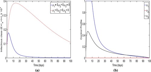
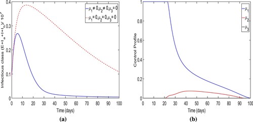
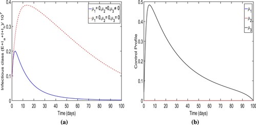
Strategy-A: The implementation of lockdown, social distancing and increase in the awareness, testing-diagnoses and intense medical care (i.e. ${\mu }_1,{\mu }_2,{\mu }_3\ne 0$). By applying this strategy, we notice that the number of people in infected classes $(E+I_a+I+I_h)$ are less rather then there is no control in place. It could be also observed that it also approaches to zero (disease almost dies out) within 90 days when control is applied (see Figure 11(a)). More precisely, we observe that this control strategy prevents almost $36.70\times {10}^7$ total infectious cases. The dynamics of control variables is presented in Figure 11(b), which reveals that ${\mu }_1$ is at its upper bound for the initially 10 days before it eventually reduces to zero. The increment is noticed in control ${\mu }_2$ to attain $45\mathrm{\%}$ of its maximum, the total infectious cases increases, and however, after the peak of infectious cases, this particular control also reduce to zero. Similarly, the control variables ${\mu }_3$ rises before falling to zero. However, the peak of control ${\mu }_3$ is very low. In Figure 11, we observe that control ${\mu }_1$ and ${\mu }_2$ is initially increasing to its peak value as the trajectory of optimal infectious cases is increasing to its peak value.

Figure 11. The trajectory of total infectious cases and control profile for the strategy A.

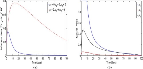
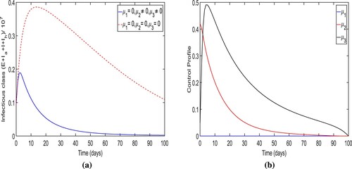
Strategy-B: The implementation of lockdown, social distancing, increase in the awareness and the enhancement in intense medical care (i.e. ${\mu }_1,{\mu }_3\ne 0,{\mu }_2=0$). The simulation results of the total number of individuals in infectious classes are depicted in Figure 12(a) when the control strategy is applied. Implementing this control strategy, it could be observed that the total number people in contagious classes $(E+I_a+I+I_h)$ in the presence of control is less than the total number individuals in contagious classes $(E+I_a+I+I_h)$ when the control is not applied. Specifically, $35.30\times {10}^7$ infection cases were averted when strategy-B is implemented. From Figures 11 and 12, we also observe that the optimal trajectories of the total number of individuals of infectious classes for strategy-A and strategy-B are almost same. Therefore, we observe that there is little effect of control ${\mu }_2$ on the optimal trajectory. 12(b) demonstrates the control profile for this control strategy. In the control profile, we also observe that the shape of two controls ${\mu }_1$ and ${\mu }_2$ is almost identical to that in strategy-A, and the control ${\mu }_3$ is zero.

Figure 12. The figure depicts the trajectories of total infectious cases and control profile for the strategy B.

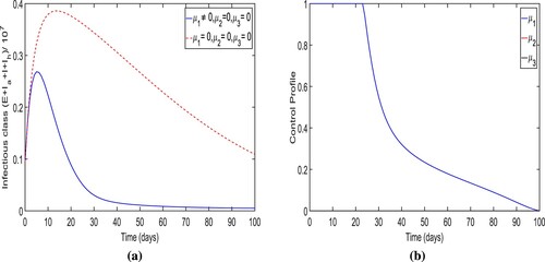
Strategy-C: The implementation of lockdown, social distancing, increase in the awareness and testing-diagnoses (i.e. ${\mu }_1,{\mu }_2\ne 0,{\mu }_3=0$). The optimal trajectory of the total number of infectious people for the controlled system (19(19) $\begin{array}{rl}\frac{\mathrm{d}{S}_u}{\mathrm{d}t}& =\mathrm{\Lambda }-\lambda (1-{\mu }_1(t))S_u-\mathrm{d}{S}_u-q{S}_u+\zeta S_q,\\ \frac{\mathrm{d}{S}_q}{\mathrm{d}t}& =q{S}_u+(1-p)(1-{\mu }_1(t))\lambda S_u-({ϵ}_q\lambda (1-{\mu }_1(t))+\zeta +d)S_q,\\ \frac{\mathrm{d}E}{\mathrm{d}t}& =p\lambda (1-{\mu }_1(t))S_u+{ϵ}_q\lambda (1-{\mu }_1(t))S_q-(\alpha +d)E,\\ \frac{\mathrm{d}{I}_a}{\mathrm{d}t}& =p_1\alpha E-({\delta }_1+{\gamma }_1+d)I_a-{\varphi }_1(1+{\mu }_2(t))I_a,\\ \frac{\mathrm{d}I}{\mathrm{d}t}& =p_2\alpha E-({\delta }_2+{\gamma }_2+d)I-{\varphi }_2(1+{\mu }_2(t))I,\\ \frac{\mathrm{d}{I}_h}{\mathrm{d}t}& =(1-p_1-p_2)\alpha E+{\varphi }_1(1+{\mu }_2(t))I_a\\ & +{\varphi }_2(1+{\mu }_2(t))I-({\delta }_3+{\gamma }_3+d)I_h-{\mu }_3(t)I_h,\\ \frac{\mathrm{d}R}{\mathrm{d}t}& ={\gamma }_1{I}_a+{\gamma }_{2}I+{\gamma }_3{I}_h+{\mu }_3(t)I_h-\mathrm{d}R,\end{array}$(19) ) when strategy-C is applied and trajectory of that for system (24(24) $\frac{\mathrm{d}x}{\mathrm{d}t}=\frac{\mathrm{\partial }H(t,x,\mu ,\mathrm{\Gamma })}{\mathrm{\partial }\mathrm{\Gamma }},0=\frac{\mathrm{\partial }H(t,x,\mu ,\mathrm{\Gamma })}{\mathrm{\partial }\mathrm{\Gamma }},\frac{\mathrm{d}\mathrm{\Gamma }}{\mathrm{d}t}=\frac{\mathrm{\partial }H(t,x,\mu ,\mathrm{\Gamma })}{\mathrm{\partial }\mathrm{\Gamma }}.$(24) ) when no control is implemented, are illustrated in Figure 13(a). It has been observed whenever this preventive technique is used, the overall number of infected individuals decreases. Particularly, $33.73\times {10}^7$ infection cases were averted when strategy C was used to control the disease. The peak for the optimal trajectory in this strategy is at 0.275 and higher than that for the strategy-B. In this control strategy, the optimal trajectory could not achieve zero level of infection as time tends to end time (100 days). The control profile figure Figure 13(b) indicates that the control ${\mu }_1$ is $100\mathrm{\%}$ effective for only 20 days initially and then reduces continuously to zero over time. However, control ${\mu }_2$ is initially in the role after 20 days and then goes to its maximum level $(7\mathrm{\%})$ and falls steadily to zero at time t = 100 days. As a result, the control ${\mu }_1$ makes the most effort in this method to lower the overall number of infected individuals.

Figure 13. The figure depicts the trajectory of total infectious cases and control profile for the case of strategy C.

Strategy-D: The enhancement in testing-diagnoses and intense medical care (i.e. ${\mu }_1=0,{\mu }_2,{\mu }_3\ne 0$). The simulation results for the total number of individuals in infectious classes in in this strategy are depicted in Figure 14(a). Here, in the presence of control, the total number of individuals in infectious classes is less than when no control measure is implemented as expected. Notably, we found that $33.33\times {10}^7$ new cases were averted when the control strategy-B was applied. The optimal trajectory for the total number of individuals in infectious classes attains its peak $(0.18)$ within initially 4–5 days. In addition, toward the end of the strategy implementation, the trajectory converges to zero. 14(b) shows the control profile for this intervention technique that indicates that the control ${\mu }_2$ gradually declines to zero. However, the control ${\mu }_3$ declines to zero after attaining its peak.

Figure 14. The figure depicts the trajectory of total infectious cases and control profile for the strategy D.

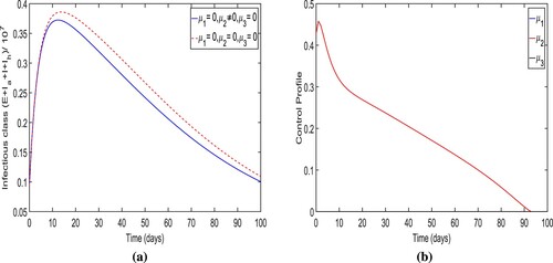
Strategy-E: The use of lockdown, social distancing and awareness only (i.e. ${\mu }_1\ne 0,{\mu }_2,{\mu }_3=0$). The simulation results for the total number of individuals in infectious classes with the implementation of this strategy are depicted in Figure 15(a). We demonstrate that when strategy E is used, the overall number of people in contagious classes is lower than when no control measures are used as expected. When the control strategy-E is used, it is found that $33.74\times {10}^7$ infection cases are avoided. The optimal trajectory for the total number of individuals in infectious classes attains its peak at $(0.27)$ within initially 4−5 days of the simulation period and converges to a positive number at the end time of the strategy implementation. The control profile for strategy-E is shown in Figure 15(b) which displays that the control variable ${\mu }_1$ is $100\mathrm{\%}$ effective with maximum efforts for only 22 days initially and then reduces continuously to zero over time.

Figure 15. The figure illustrates the optimal trajectory of total infectious cases and control profile for control strategy E.

Strategy-F: The enhancement in testing-diagnoses only (i.e. ${\mu }_1,{\mu }_3=0,{\mu }_2\ne 0$). The optimal trajectory of the total number of infectious individuals for the controlled system (19(19) $\begin{array}{rl}\frac{\mathrm{d}{S}_u}{\mathrm{d}t}& =\mathrm{\Lambda }-\lambda (1-{\mu }_1(t))S_u-\mathrm{d}{S}_u-q{S}_u+\zeta S_q,\\ \frac{\mathrm{d}{S}_q}{\mathrm{d}t}& =q{S}_u+(1-p)(1-{\mu }_1(t))\lambda S_u-({ϵ}_q\lambda (1-{\mu }_1(t))+\zeta +d)S_q,\\ \frac{\mathrm{d}E}{\mathrm{d}t}& =p\lambda (1-{\mu }_1(t))S_u+{ϵ}_q\lambda (1-{\mu }_1(t))S_q-(\alpha +d)E,\\ \frac{\mathrm{d}{I}_a}{\mathrm{d}t}& =p_1\alpha E-({\delta }_1+{\gamma }_1+d)I_a-{\varphi }_1(1+{\mu }_2(t))I_a,\\ \frac{\mathrm{d}I}{\mathrm{d}t}& =p_2\alpha E-({\delta }_2+{\gamma }_2+d)I-{\varphi }_2(1+{\mu }_2(t))I,\\ \frac{\mathrm{d}{I}_h}{\mathrm{d}t}& =(1-p_1-p_2)\alpha E+{\varphi }_1(1+{\mu }_2(t))I_a\\ & +{\varphi }_2(1+{\mu }_2(t))I-({\delta }_3+{\gamma }_3+d)I_h-{\mu }_3(t)I_h,\\ \frac{\mathrm{d}R}{\mathrm{d}t}& ={\gamma }_1{I}_a+{\gamma }_{2}I+{\gamma }_3{I}_h+{\mu }_3(t)I_h-\mathrm{d}R,\end{array}$(19) ) is shown in Figure 16(a) when the augmentation in testing-diagnoses only is taken as a control measure. We can see that when strategy-F is used to reduce the infection cases, the overall number of individuals in contagious classes is less than if no precautions are used as intended. $2.88\times {10}^7$ new cases were avoided by applying the strategy. In comparison to the other six control strategies, there are extremely few cases of infection avoided. Within the first 15–20 days, the ideal trajectory for the total number of individuals in infectious classes reaches its maximum at $(0.38\times {10}^7)$. It also noted that the trajectory converges to a large positive number at the final time of the strategy implementation. The control profile for this intervention scenario is given in Figure 16(b) displays that the variable ${\mu }_2$ gradually reduces to zero over time.

Figure 16. The figure determines the optimal trajectory of total infectious cases and control profile for intervention strategy G.

Strategy-G: The intense medical care only (i.e. ${\mu }_1,{\mu }_2=0,{\mu }_3\ne 0$). The simulation results of the optimal trajectory of the overall infected individuals and control profile for the control system when the control strategy-G is applied are presented in Figure 17. We observe that when the control strategy-G is applied, the total number of people of infectious classes is less than when no control measure is used as expected. It also noted that its trajectory converges to almost zero level at the final time of the strategy implementation. More precisely, we observe that $32.60\times {10}^7$ new cases were prevented when the control strategy-G is applied. The optimal trajectory for the total number of individuals in infectious classes attains its peak $(0.20)$ within initially 2–3 days. It is a smaller peak of infectious cases than that for no control measure is applied. The control profile for this intervention strategy is presented in Figure 17(b) which illustrates that the control ${\mu }_3$ attains its peak value within initially 5−6 days and then gradually reduces to zero over time.

Figure 17. The figure illustrates the trajectories of total infectious cases and control profile for control strategy G.

5.2. Cost-effective analysis

To eradicate or control COVID-19 infections in a community, it might be time-consuming, costly, or both. As a result, conducting a cost-benefit analysis is critical. In this part of the study, we try to figure out the most cost-effective intervention in India's fight against COVID-19. Here, we explore the cost-effective analysis based on the numerical implementation of the optimal system shown in Section 5. We compute the cost-effectiveness of protective measure related to the use of three considered time-dependent control variables ${\mu }_1(t),{\mu }_2(t)$ and ${\mu }_3(t).$ The cost benefits associated with applied the interventions can be compared through cost-effectiveness analysis. We investigated seven control strategies for the practice of time-dependent control variables ${\mu }_1(t),{\mu }_2(t),$ and ${\mu }_3(t)$ in various combination for cost-effective study as discussed in Section 5.1.

We employ three ways to execute the cost-effective analysis: the Infection Averted Ratio (IAR), the Average Cost-Effective Ratio (ACER), and the Incremental Cost-Effective Ratio (ICER). The three cost-effective approaches [1, 54] are as follows:

Infection Averted Ratio (IAR): The strategy with highest value of IAR is the most effective strategy according to IAR analysis. IAR is given by: $\mathrm{IAR}=\frac{\text{Cumulative infection averted}}{\text{Cumulative recoveries}}.$ For the considered parametric values, the IAR for the different optimal interventions has been computed and presented in Table 5. In  18, we easily compare the values of IAR for different control strategies. Strategy-A containing the all three control measures, generates the highest IAR ratio. Hence, it is the most effective according to IAR analysis. Strategy-A is preceded by strategy-B. It is also observed that Strategy-A, Strategy-B, Strategy-C, and Strategy-E have the high values of IAR.

Figure 18. The figure depicts the IAR for all seven optimal control strategies.

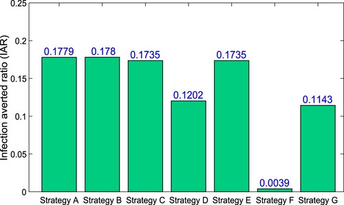
Table 5. Control measures with increasing order of total infection cases avoided.

Strategy	Total infection averted	Total cost	IAR	ACER
$F:{\mu }_2\ne 0$	$2.88\times {10}^7$	35.0031	0.0039	$1.21\times {10}^{-6}$
$G:{\mu }_3\ne 0$	$32.60\times {10}^7$	35.4920	0.1143	$1.08\times {10}^{-7}$
$D:{\mu }_2,{\mu }_3\ne 0$	$33.33\times {10}^7$	40.4781	0.1202	$1.21\times {10}^{-7}$
$C:{\mu }_1,{\mu }_2\ne 0$	$33.73\times {10}^7$	23.9467	0.1735	$7.10\times {10}^{-8}$
$E:{\mu }_1\ne 0$	$33.74\times {10}^7$	20.6084	0.1735	$6.11\times {10}^{-8}$
$B:{\mu }_1,{\mu }_3\ne 0$	$36.66\times {10}^7$	35.3076	0.1780	$9.63\times {10}^{-7}$
$A:{\mu }_1,{\mu }_2,{\mu }_3\ne 0$	$36.70\times {10}^7$	36.7240	0.1779	$1\times {10}^{-7}$

Average Cost-Effectiveness Ratio (ACER): This is determined by evaluating the variation in the number of infections avoided and the cost of control techniques used. ACER is concerned with a single intervention technique and its comparison to a baseline alternative. As a result, the average cost-effectiveness ratio (ACER) is calculated using the following mathematical formula against one of the worst case of no control (i.e. ${\mu }_1={\mu }_2={\mu }_3=0$). $\mathrm{ACER}=\frac{\text{Total cost invested on the intervention}}{\text{Total number of infections averted using the intervention}}.$ The overall number of infections prevented is computed using the formula ${\int }_0^T\tilde{F}\mathrm{d}t-{\int }_0^{T}F\mathrm{d}t$, where $\tilde{F}$ is the solution for total number of infected people without controls and F is the optimal solution for total number of individuals in infection classes with controls [1]. The cost function TC provided by (20(20) $TC={\int }_0^T\frac{1}{2}(c_1{\mu }_1^2+c_2{\mu }_2^2+c_3{\mu }_3^2)\mathrm{d}t,$(20) ) is used to compute the cost of the intervention. As per this method of cost analysis, the most cost-effective intervention is the one with the lowest ACER value [54].

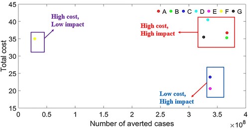
The ACER value for the various intervention strategies is given in Table 5 and  19. As shown in 19, Strategy-E has the lowest ACER value, following by Strategy-C, then Strategy-A. These results can be also observed in Table 5. As a result, the most adequate control strategy-E, followed by strategy-C, and then strategy-A, per the ACER cost benefit analysis.  20 shows the comparison of all intervention strategies in terms of total cost and number of averted cases.

Figure 19. The figure shows the ACER for all seven optimal control strategies.

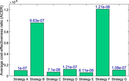
Figure 20. Comparison of all intervention strategies in terms of total cost and number of averted cases.

Incremental Cost-Effectiveness Ratio (ICER): The goal of ICER is to compare the cost and healthcare outcomes of two different control measures. It is the ratio of the cost difference between two distinct strategies to the overall number of infections prevented. On the other hand, performing a cost-benefit comparison between two alternative control systems is useful. The following mathematical phrase is used to calculate ICER: $\mathrm{ICER}=\frac{\text{Difference between the costs for employing strategies }\mathbf{m}\text{ and }\mathbf{n}}{\begin{array}{c}\text{Variation in the number of infections avoided as a result of}\\ \text{employing strategies }\mathbf{m}\text{ and }\mathbf{n}\end{array}}.$ The cost involved in the implementation of a specific strategy is calculated using the expression that can be seen in Equations (20(20) $TC={\int }_0^T\frac{1}{2}(c_1{\mu }_1^2+c_2{\mu }_2^2+c_3{\mu }_3^2)\mathrm{d}t,$(20) ). Further, the ICER for strategy-F (the enhancement in the testing diagnosis, only i.e. ${\mu }_2\ne 0$) and strategy-G (the intense medical care, only i.e. ${\mu }_3\ne 0$ ) are computed, as follows. $\begin{array}{rl}\mathrm{ICER}(\mathrm{F})& =\frac{35.0031}{2.88\times {10}^7}=1.21\times {10}^{-6},\\ \mathrm{ICER}(\mathrm{G})& =\frac{35.4920-35.0031}{32.60\times {10}^7-2.88\times {10}^7}=1.65\times {10}^{-9}.\end{array}$ Comparing ICER(F) and ICER(G), it is observed that ICER(F) is higher than ICER(G). Therefore, we conclude that strategy F is more costly and less effective in controlling the disease compared to strategy G. Hence, strategy F is removed from proceeding analysis of cost-effectiveness based on ICER computations, shown in Table 6. Further, we shall compare strategies G and D.

Table 6. ICER computations for strategies F and G.

Strategy	Total infection averted	Total cost	ACER	ICER
F	$2.88\times {10}^7$	35.0031	$1.21\times {10}^{-6}$	$1.21\times {10}^{-6}$
G	$32.60\times {10}^7$	35.4920	$1.08\times {10}^{-7}$	$1.64\times {10}^{-9}$

Now, the ICER for strategy G (the intense medical care, only i.e.${\mu }_3\ne 0$) and strategy D (the enhancement in testing-diagnoses and intense medical care, i.e. ${\mu }_2,{\mu }_3\ne 0$) are computed $\begin{array}{rl}\mathrm{ICER}(\mathrm{G})& =\frac{35.4920}{32.60\times {10}^7}=1.08\times {10}^{-7},\\ \mathrm{ICER}(\mathrm{D})& =\frac{40.4781-35.4920}{33.33\times {10}^7-32.60\times {10}^7}=6.83\times {10}^{-7}.\end{array}$ When ICER(G) and ICER(D) are compared, ICER(D) is found to be greater than ICER(G). As a result, strategy D is more expensive and far less productive than strategy G. Hence, strategy D is eliminated from the following cost-effectiveness analysis relying on ICER estimates, as shown in Table 7. We will also compare strategies G and C. The ICER for strategies G and C is calculated as $\begin{array}{rl}\mathrm{ICER}(\mathrm{G})& =\frac{35.4920}{32.60\times {10}^7}=1.08\times {10}^{-7},\\ \mathrm{ICER}(\mathrm{C})& =\frac{23.9467-35.4920}{33.73\times {10}^7-32.60\times {10}^7}=-1.58\times {10}^{-6}.\end{array}$ The ICER for strategy C is smaller than that of strategy G, indicating that strategy C is less expensive and more successful than strategy G. As a result, strategy G is no longer used in further ICER computations. Table 8 shows the ICER comparison for strategies G and C. We'll now contrast strategies C and E. The ICER for strategy C and E are given by $\begin{array}{rl}\mathrm{ICER}(\mathrm{C})& =\frac{23.9467}{33.73\times {10}^7}=7.10\times {10}^{-8},\\ \mathrm{ICER}(\mathrm{E})& =\frac{20.6084-23.9467}{33.74\times {10}^7-33.73\times {10}^7}=-3.33\times {10}^{-5}.\end{array}$ Here, we have that ICER(C) is bigger than ICER(E). As a result, strategy C is both more expensive and ineffective than strategy E. Table 9 represents the comparison for strategies E and C. In the following ICER computations, strategy E is employed instead of strategy C.

We shall now compare strategies E and B. The ICER for strategy E and strategy B are given as follow $\begin{array}{rl}\mathrm{ICER}(\mathrm{E})& =\frac{20.6084}{33.74\times {10}^7}=6.11\times {10}^{-8},\\ \mathrm{ICER}(\mathrm{B})& =\frac{35.3076-20.6084}{36.66\times {10}^7-33.74\times {10}^7}=5.03\times {10}^{-7}.\end{array}$ Here, we notice that ICER(E)<ICER(B). Therefore, strategy E is better than strategy B. Hence, strategy B is removed from subsequent ICER computations. The comparison of ICER for strategies E and B is shown in Table 10.

Table 7. ICER computations for strategies D and G.

Strategy	Total infection averted	Total cost	ACER	ICER
G	$32.60\times {10}^7$	35.4920	$1.08\times {10}^{-7}$	$1.08\times {10}^{-7}$
D	$33.33\times {10}^7$	40.4781	$1.21\times {10}^{-7}$	$6.83\times {10}^{-7}$

Table 8. ICER computations for strategies C and G.

Strategy	Total infection averted	Total cost	ACER	ICER
G	$32.60\times {10}^7$	35.4920	$1.08\times {10}^{-7}$	$1.08\times {10}^{-7}$
C	$33.73\times {10}^7$	23.9467	$7.10\times {10}^{-8}$	$-1.58\times {10}^{-6}$

Table 9. ICER computations for strategies E and C.

Strategy	Total infection averted	Total cost	ACER	ICER
C	$33.73\times {10}^7$	23.9467	$7.10\times {10}^{-8}$	$7.10\times {10}^{-8}$
E	$33.74\times {10}^7$	20.6084	$6.11\times {10}^{-8}$	$-3.33\times {10}^{-8}$

Table 10. ICER computations for strategies E and B.

Strategy	Total infection averted	Total cost	ACER	ICER
E	$33.74\times {10}^7$	20.6084	$6.11\times {10}^{-8}$	$6.11\times {10}^{-8}$
B	$36.66\times {10}^7$	35.3076	$9.63\times {10}^{-7}$	$5.03\times {10}^{-7}$

Further, we compare strategy E and A. The ICER for strategy E and strategy A are given as follow $\begin{array}{rl}\mathrm{ICER}(\mathrm{E})& =\frac{20.6084}{33.74\times {10}^7}=6.11\times {10}^{-8},\\ \mathrm{ICER}(\mathrm{A})& =\frac{36.7240-20.6084}{36.70\times {10}^7-33.74\times {10}^7}=5.44\times {10}^{-7}.\end{array}$ In Table 11, it is observed that ICER(A)>ICER(E). As a result, strategy A is much more expensive and impractical than strategy E. Thus, we conclude that strategy E is perhaps the most cost-effective in reducing the COVID-19 in India based on cost analysis and ICER values for various strategies.

6. Discussion and conclusion

The coronavirus disease 2019 (COVID-19) pandemic has established significant public health challenges and initiated a substantial economic burden worldwide. However, the employment of numerous non-pharmaceutical interventions (NPIs), contact tracing, isolation, quarantine, and wearing face masks, are still playing significant role in controlling the pandemic. In order to acquire a better knowledge of how the disease spreads and to research potential preventative and control measures to limit the population's disease transmission flow, a mathematical study of the transmission dynamics of the unique COVID-19 pandemic has been presented. In this study, we used a deterministic epidemic model to investigate the transmission dynamics of coronavirus in India, and then analysed it to see how beneficial face masks, isolation, and quarantine are at controlling the disease.

Table 11. ICER computations for strategies E and A.

Strategy	Total infection averted	Total cost	ACER	ICER
E	$33.74\times {10}^7$	20.6084	$6.11\times {10}^{-8}$	$6.11\times {10}^{-8}$
A	$36.70\times {10}^7$	36.7240	$1\times {10}^{-7}$	$5.44\times {10}^{-7}$

The basic reproduction number $(R_0)$ and equilibria for the proposed model system (disease-free and endemic equilibrium) have been computed. The local stability of disease-free equilibrium has been discussed when $R_0$ is less than one. Also, the global stability of disease-free equilibrium in the case of perfect quarantine of susceptible individuals $({ϵ}_q=0)$ has been established in case of $R_0<1.$ Interestingly, the occurrence of backward bifurcation at $R_0=1$ has been demonstrated in case of imperfect quarantine of susceptible individuals $({ϵ}_q\ne 0)$. Consequently, the existence of multiple endemic equilibria has been confirmed in case of imperfect quarantine of susceptible individuals $({ϵ}_q\ne 0)$ when $R_0<1.$ As a result, the condition $R_0<1$ is insufficient for the disease eradication from the community in case of imperfect quarantine of susceptible individuals $({ϵ}_q\ne 0)$. Rajput et al. [58] also reached a similar finding, however they obtained the result for vaccine effectiveness. Hence, for the eradication of the disease, it is important to have perfect quarantine facilities, and people must be aware and motivated about effective quarantine. In the present scenario, this particular result becomes rather more significant because of high transmission rate. Moreover, the threshold dynamics of $R_0$ corresponding to control measures such as quarantine and isolation have been investigated in order to determine how much control measure is required for a favourable impact.

Using publicly available data sources, the model output is fitted to cumulative confirmed COVID-19 cases for India from September 1, 2020 to December 31, 2020. The fitting was done in MATLAB using the MCMC approach. The empirical data sets were used to estimate parameters such as the COVID-19 effective contact rate $(\beta )$ and the proportion of people who protect their faces with a mask in public places $(p_M)$. The estimated values of β and $p_M$ are presented in Table 2 and model fitting of model output to number of cumulative cases is shown in 3. Further, we have presented the numerical simulation to validate the obtained theoretical results. The local stability of the equilibria (disease-free and endemic equilibrium) has been validated numerically in 4–6. The local sensitivity (using normalized forward sensitivity index) and global sensitivity (using PRCC analysis) of basic reproduction number are shown in 7 and 8, respectively. From threshold dynamics of the basic reproduction number ( 9), we found that the infectivity of isolated infected individuals should be maintained below its threshold value for the successful isolation program. To lessen the COVID-19 load in India, sanitary quarantine and efficient isolation will be appropriate protection measures. As a result, we conclude that in order to reduce COVID-19 transmission, the $R_0$ must be kept below unity, which can be accomplished by maintaining public use of face masks, lowering infectivity, and improving contact tracing of isolated infected individuals with high quarantine efficiency.

In order to establish the most cost-effective control strategy, an optimal control problem for the proposed system was formulated and evaluated. The first preventive measures, such as lock-down, social distancing, and awareness, are considered control methods; the second, testing-diagnosis for exposed individuals; and the third, intense medical care, are considered control ways to assess the optimal control problem. The appropriate conditions for optimal control and the optimality system are determined using Pontryagin's Principle. For the best control model, various control strategies were investigated and simulated. The highlights of numerical evaluations demonstrate that:

• Strategy A, which implements COVID-19 infection control (lockdown, social distancing and enhanced awareness, testing diagnostics, and intensive medical care), prevents the greatest number of infection cases of any of the applied control measures. This is seen in Figure 11, which shows that a total of $36.70\times {10}^7$ new infection cases were avoided.

• Strategy E employing control (the use of lockdown, social distancing, and awareness only) against COVID-19 disease is the most cost-effective way to control the infection as presented in Section 5.2. Strategy E also has the least value of ACER (refer the Table 5) and associated cost calculated by (20(20) $TC={\int }_0^T\frac{1}{2}(c_1{\mu }_1^2+c_2{\mu }_2^2+c_3{\mu }_3^2)\mathrm{d}t,$(20) ).

• Strategy C includes the implementation of lockdown, social distancing, awareness, and enhancement in testing diagnoses (i.e.${\mu }_1,{\mu }_2\ne 0$) is the second most cost-effective in controlling the current COVID-19 pandemic.

The above findings of our study are different from the previous studies [10, 54] in the context of cost-effectiveness of different intervention strategies. Given the foregoing, it is reasonable to conclude that two important characteristics govern the flattening of the novel coronavirus infection curve: the effective transmission factor and the capacity to identify infectious persons. There must be efforts made to reduce transmission rates and to improve detection of infectious cases in order to avoid undesired interactions with contagious individuals in order to assure an infection-free region. If strict compliance is maintained, transmission paths from symptomatic, asymptomatic, and hospitalized patients will be actively prevented, and hospitalized people with severe COVID-19 symptoms will have access to supplemental oxygen or mechanical breathing. In stopping the spread of the novel coronavirus, it is also necessary to enhance diagnostic accuracy for the detection and fast treatment of asymptomatic persons. It is also worth highlighting that health services should be expanded and better equipped to deal with the growing number of cases and effectively manage those who develop difficulties as a result of the COVID-19 infection. As a result, it can be concluded that the transmission of COVID-19 disease can be controlled while minimizing the cost of non-pharmaceutical precautions if quarantine and isolation are increased significantly, and all quarantined and non-quarantined people must adhere to all non-pharmaceutical precautionary measures as prescribed by health care authorities. The success of optimal control techniques is largely dependent on infectives and proper implementation of government regulations by the health-care authorities.

The fight against COVID-19 transmission takes a multi-pronged approach. Other control variables, such as personal hygiene and control for different variations, have not yet been examined in this study, leaving the door open for future investigation. The findings of this study can serve as a significant resource for the COVID-19 Local National Control Program, as well as a foundation for the development and implementation of the best intervention policies to combat the new COVID-19 variations.

Disclosure statement

No potential conflict of interest was reported by the author(s).

Additional information

Funding

Vijay Pal Bajiya receives funding as senior research fellowship from the Council of Scientific & Industrial Research (CSIR), India (File No. 09/1131(0006)/2017-EMR-I). The research work of Sarita Bugalia is supported by the CSIR, India (File No. 09/1131(0025)/2018-EMR-I). The research work of Jai Prakash Tripathi is supported by the Science and Engineering Research Board (SERB), India (File No. ECR/2017/002786).

References

- F.B. Agusto and I.M. ELmojtaba, Optimal control and cost-effective analysis of malaria/visceral leishmaniasis co-infection, PLoS. One. 12(2) (2017), p. e0171102.
- A.E. Aiello, G.F. Murray, V. Perez, R.M. Coulborn, B.M. Davis, M. Uddin, D.K. Shay, S.H. Waterman, and A.S. Monto, Mask use, hand hygiene, and seasonal influenza-like illness among young adults: A randomized intervention trial, J. Infect. Dis. 201(4) (2010), pp. 491–498.
- A.E. Aiello, V. Perez, R.M. Coulborn, B.M. Davis, M. Uddin, and A.S. Monto, Facemasks, hand hygiene, and influenza among young adults: A randomized intervention trial, PLoS. One. 7(1) (2012), pp. e29744.
- R.M. Anderson, H. Heesterbeek, D. Klinkenberg, and T.D. Hollingsworth, How will country-based mitigation measures influence the course of the COVID-19 epidemic?, The Lancet 395(10228) (2020), pp. 931–934.
- E.F. Arruda, D.H. Pastore, C.M. Dias, and S.S. Das, Modelling and optimal control of multi strain epidemics, with application to COVID-19, arXiv preprint arXiv:2101.08137 (2021).
- J.K.K. Asamoah, F. Nyabadza, Z. Jin, E. Bonyah, M.A. Khan, M.Y. Li, and T. Hayat, Backward bifurcation and sensitivity analysis for bacterial meningitis transmission dynamics with a nonlinear recovery rate, Chaos, Solitons Fract. 140 (2020), pp. 110237.
- J.K.K. Asamoah, M.A. Owusu, Z. Jin, F.T. Oduro, A. Abidemi, and E.O. Gyasi, Global stability and cost-effectiveness analysis of COVID-19 considering the impact of the environment: Using data from Ghana, Chaos Solitons Fract. 140 (2020), pp. 110103.
- J.K.K. Asamoah, Z. Jin, and G.-Q. Sun, Non-seasonal and seasonal relapse model for Q fever disease with comprehensive cost-effectiveness analysis, Res. Phys. 22 (2021), p. 103889.
- J.K.K. Asamoah, Z. Jin, G.-Q. Sun, B. Seidu, E. Yankson, A. Abidemi, F.T. Oduro, S.E. Moore, and E. Okyere, Sensitivity assessment and optimal economic evaluation of a new COVID-19 compartmental epidemic model with control interventions, Chaos, Solitons Fract. 146 (2021), pp. 110885.
- J.K.K. Asamoah, E. Okyere, A. Abidemi, S.E. Moore, G.-Q. Sun, Z. Jin, E. Acheampong, and J.F. Gordon, Optimal control and comprehensive cost-effectiveness analysis for COVID-19, Res. Phys. (2022), pp. 105177.
- Y. Bai, L. Yao, T. Wei, F. Tian, D.-Y. Jin, L. Chen, and M. Wang, Presumed asymptomatic carrier transmission of COVID-19, JAMA 323(14) (2020), pp. 1406–1407.
- V.P. Bajiya, S. Bugalia, and J.P. Tripathi, Mathematical modeling of COVID-19: Impact of non-pharmaceutical interventions in India, Chaos Interdisci. J. Nonlinear Sci. 30(11) (2020), p. 113143.
- V.P. Bajiya, J. Prakash Tripathi, and R. Kumar Upadhyay, Deciphering dynamics of recent COVID-19 outbreak in India: An age-structured modeling, arXiv preprint arXiv:2201.09803 (2022).
- S.R. Bandekar and M. Ghosh, Mathematical modeling of COVID-19 in India and its states with optimal control, Model. Earth. Syst. Environ. (2021), pp. 1–16.
- H. Behncke, Optimal control of deterministic epidemics, Optim. Control Appl. Methods 21(6) (2000), pp. 269–285.
- S. Biswas, A. Subramanian, I.M. ELMojtaba, J. Chattopadhyay, and R.R. Sarkar, Optimal combinations of control strategies and cost-effective analysis for visceral leishmaniasis disease transmission, PLoS. One. 12(2) (2017), p. e0172465.
- K.W. Blayneh, A.B. Gumel, S. Lenhart, and T. Clayton, Backward bifurcation and optimal control in transmission dynamics of West Nile virus, Bull. Math. Biol. 72(4) (2010), pp. 1006–1028.
- M.C.J. Bootsma and N.M. Ferguson, The effect of public health measures on the 1918 influenza pandemic in US cities, Proc. Nat. Acad. Sci. 104(18) (2007), pp. 7588–7593.
- S. Bugalia, V.P. Bajiya, J.P Tripathi, M.-T. Li, and G.-Q. Sun, Mathematical modeling of COVID-19 transmission: The roles of intervention strategies and lockdown, Math. Biosci. Eng. 17(5) (2020), pp. 5961–5986.
- J. Carr, Applications of Centre Manifold Theory, Springer Science & Business Media, New York, Vol. 35, 2012.
- C. Castillo-Chavez and B. Song, Dynamical models of tuberculosis and their applications, Math. Biosci. Eng. 1(2) (2004), pp. 361.
- C. Castillo-Chavez, Z. Feng, and W. Huang, On the computation of R0 and its role in global stability, IMA Vol. Math. Appl. 125 (2002), pp. 229–250.
- S. Choi and E. Jung, Optimal tuberculosis prevention and control strategy from a mathematical model based on real data, Bull. Math. Biol. 76(7) (2014), pp. 1566–1589.
- B.J. Cowling, K.-H. Chan, V.J. Fang, C.K.Y. Cheng, R.O.P. Fung, W. Wai, J. Sin, W.H. Seto, R. Yung, D.W. Chu, and B.C. Chiu, Facemasks and hand hygiene to prevent influenza transmission in households: A cluster randomized trial, Ann. Intern. Med. 151(7) (2009), pp. 437–446.
- A. Dénes and A.B. Gumel, Modeling the impact of quarantine during an outbreak of Ebola virus disease, Infect. Dis. Model. 4 (2019), pp. 12–27.
- E.X. DeJesus and C. Kaufman, Routh-Hurwitz criterion in the examination of eigenvalues of a system of nonlinear ordinary differential equations, Phys. Rev. A. 35(12) (1987), pp. 5288.
- C. Del Rio and P.N. Malani, COVID-19–new insights on a rapidly changing epidemic, JAMA 323(14) (2020), pp. 1339–1340.
- K.V. Driessche, N. Hens, P. Tilley, B.S. Quon, M.A. Chilvers, R. de Groot, M.F. Cotton, B.J. Marais, D.P. Speert, and J.E.A. Zlosnik, Surgical masks reduce airborne spread of Pseudomonas aeruginosa in colonized patients with cystic fibrosis, Am. J. Respir. Crit. Care. Med. 192(7) (2015), pp. 897–899.
- S.E. Eikenberry, M. Mancuso, E. Iboi, T. Phan, K. Eikenberry, Y. Kuang, E. Kostelich, and A.B. Gumel, To mask or not to mask: Modeling the potential for face mask use by the general public to curtail the COVID-19 pandemic, Infect. Dis. Model. 5 (2020), pp. 293–308.
- E.H. Elbasha and A.B. Gumel, Theoretical assessment of public health impact of imperfect prophylactic HIV-1 vaccines with therapeutic benefits, Bull. Math. Biol. 68(3) (2006), pp. 577.
- European Centre for Disease Prevention and Control, Control, Situation update worldwide, ECDC (2020) Available at https://www.ecdc.europa.eu/en/geographical-distribution-2019-ncov-cases. (Accessed 18 March 2020).
- N. Ferguson, D. Laydon, G. Nedjati-Gilani, N. Imai, K. Ainslie, M. Baguelin, S. Bhatia, A. Boonyasiri, Z.U.L.M.A. Cucunuba Perez, G. Cuomo-Dannenburg, and A. Dighe, Report 9: Impact of non-pharmaceutical interventions (NPIs) to reduce COVID19 mortality and healthcare demand, Imperial College Lond. 10(77482) (2020), pp. 491–497.
- W.H. Fleming and R.W. Rishel, Deterministic and Stochastic Optimal Control, Springer Science and Business Media, Vol. 1., 2012.
- P. French, In the 1918 flu pandemic, not wearing a mask was illegal in some parts of america, What Changed? CNN website (cnn.com). [Assessed on April 8, 2020] (2020).
- H. Gaff and E. Schaefer, Optimal control applied to vaccination and treatment strategies for various epidemiological models, Math. Biosci. Eng. 6(3) (2009), pp. 469.
- D. Gamerman and H.F. Lopes, Markov Chain Monte Carlo: Stochastic Simulation for Bayesian Inference, CRC Press, 2006.
- S.M. Garba, A.B. Gumel, and M.R. Abu Bakar, Backward bifurcations in dengue transmission dynamics, Math. Biosci. 215(1) (2008), pp. 11–25.
- P.A. González-Parra, S. Lee, L. Velázquez, and C. Castillo-Chavez, A note on the use of optimal control on a discrete time model of influenza dynamics, Math. Biosci. Eng. 8(1) (2011), pp. 183.
- D.F. Gudbjartsson, A. Helgason, H. Jonsson, O.T. Magnusson, P. Melsted, G.L. Norddahl, J. Saemundsdottir, A. Sigurdsson, P. Sulem, A.B. Agustsdottir, and B. Eiriksdottir, Spread of SARS-CoV-2 in the Icelandic population, N. Eng. J. Med. 382(24) (2020), pp. 2302–2315.
- H. Haario, M. Laine, A. Mira, and E. Saksman, DRAM: Efficient adaptive MCMC, Stat. Comput. 16(4) (2006), pp. 339–354.
- W.O. Kermack and A.G. McKendrick, A contribution to the mathematical theory of epidemics, Proc. R. Soc. Lond. Ser. A Contain. Papers Math. Phys. Char. 115(772) (1927), pp. 700–721.
- J.T.F. Lau, H. Tsui, M. Lau, and X. Yang, SARS transmission, risk factors, and prevention in Hong Kong, Emerging. Infect. Dis. 10(4) (2004), pp. 587.
- S.A. Lauer, K.H. Grantz, Q. Bi, F.K. Jones, Q. Zheng, H.R. Meredith, A.S. Azman, N.G. Reich, and J. Lessler, The incubation period of coronavirus disease 2019 (COVID-19) from publicly reported confirmed cases: Estimation and application, Ann. Intern. Med. 172(9) (2020), pp. 577–582.
- S. Lenhart and J.T. Workman, Optimal Control Applied to Biological Models, Chapman and Hall/CRC, New York, 2007.
- Q. Li, X. Guan, P. Wu, X. Wang, L. Zhou, Y. Tong, R. Ren, K.S. Leung, E.H. Lau, J.Y. Wong, and X. Xing, Early transmission dynamics in Wuhan, China, of novel coronavirus-infected pneumonia, N. Engl. J. Med. 382 (2020), pp. 1199–1207.
- R. Li, S. Pei, B. Chen, Y. Song, T. Zhang, W. Yang, and J. Shaman, Substantial undocumented infection facilitates the rapid dissemination of novel coronavirus (SARS-CoV-2), Science 368(6490) (2020), pp. 489–493.
- B. Luckingham, To mask or not to mask: A note on the 1918 Spanish influenza epidemic in Tucson, J. Ariz. Hist. (1984), pp. 191–204.
- C.R. MacIntyre, S. Cauchemez, D.E. Dwyer, H. Seale, P. Cheung, G. Browne, M. Fasher, J. Wood, Z. Gao, R. Booy, and N. Ferguson, Face mask use and control of respiratory virus transmission in households, Emerging. Infect. Dis. 15(2) (2009), pp. 233.
- M. Martcheva, Control strategies, in An Introduction to Mathematical Epidemiology, Springer, Boston, MA, 2015, pp. 215–248.
- R.L. Miller Neilan, E. Schaefer, H. Gaff, K. Renee Fister, and S. Lenhart, Modeling optimal intervention strategies for cholera, Bull. Math. Biol. 72(8) (2010), pp. 2004–2018.
- K. Mizumoto and G. Chowell, Transmission potential of the novel coronavirus (COVID-19) onboard the diamond Princess Cruises Ship, 2020, Infect. Dis. Model. 5 (2020), pp. 264–270.
- National Academies of Sciences, Engineering, and Medicine, Rapid expert consultation on the effectiveness of fabric masks for the COVID-19 Pandemic (April 8, 2020), in Rapid Expert Consultations on the COVID-19 Pandemic: March 14, 2020–April 8, 2020, National Academies Press (US), 2020.
- C.N. Ngonghala, E. Iboi, S. Eikenberry, M. Scotch, C.R. MacIntyre, M.H. Bonds, and A.B. Gumel, Mathematical assessment of the impact of non-pharmaceutical interventions on curtailing the 2019 novel Coronavirus, Math. Biosci. 325 (2020), pp. 108364.
- S. Olaniyi, O.S. Obabiyi, K.O. Okosun, A.T. Oladipo, and S.O. Adewale, Mathematical modelling and optimal cost-effective control of COVID-19 transmission dynamics, Euro. Phys. J. Plus 135(11) (2020), pp. 1–20.
- T.A. Perkins and G. España, Optimal control of the COVID-19 pandemic with non-pharmaceutical interventions, Bull. Math. Biol. 82(9) (2020), pp. 1–24.
- O.J. Peter, A.I. Abioye, F.A. Oguntolu, T.A. Owolabi, M.O. Ajisope, A.G. Zakari, and T.G. Shaba, Modelling and optimal control analysis of Lassa fever disease, Inform. Med. Unlocked 20 (2020), p. 100419.
- L.S. Pontryagin, V.G. Boltyanskii, R.V. Gamkrelidze, and E.F. Mishchenko, The Mathematical Theory of Optimal Processes, The Maximum Principle, John Wiley and Sons, New York, 1962.
- A. Rajput, M. Sajid, C. Shekhar, and R. Aggarwal, Optimal control strategies on COVID-19 infection to bolster the efficacy of vaccination in India, Sci. Rep. 11(1) (2021), pp. 1–18.
- J.P. Romero-Leiton, J.M. Montoya-Aguilar, and E. Ibargüen-Mondragón, An optimal control problem applied to malaria disease in Colombia, Appl. Math. Sci. 12(6) (2018), pp. 279–292.
- N.R. Sasmita, M. Ikhwan, S. Suyanto, and V. Chongsuvivatwong, Optimal control on a mathematical model to pattern the progression of coronavirus disease 2019 (COVID-19) in Indonesia, Global Health Res. Policy 5(1) (2020), pp. 1–12.
- E. Shim, Optimal strategies of social distancing and vaccination against seasonal influenza, Math. Biosci. Eng. 10(5 & 6) (2013), pp. 1615.
- W.K. Silverstein, L. Stroud, G.E. Cleghorn, and J.A. Leis, First imported case of 2019 novel coronavirus in Canada, Present. Mild Pneumonia Lancet 395(10225) (2020), pp. 734.
- R.E. Stockwell, M.E. Wood, C. He, L.J. Sherrard, E.L. Ballard, T.J. Kidd, G.R. Johnson, L.D. Knibbs, and S.C. Bell, Face masks reduce the release of Pseudomonas aeruginosa cough aerosols when worn for clinically relevant periods, Am. J. Respir. Crit. Care. Med. 198(10) (2018), pp. 1339–1342.
- B. Tang, X. Wang, Q. Li, N.L. Bragazzi, S. Tang, Y. Xiao, and J. Wu, Estimation of the transmission risk of the 2019-nCoV and its implication for public health interventions, J. Clin. Med. 9(2) (2020), p. 462.
- J.M. Tchuenche, S.A. Khamis, F.B. Agusto, and S.C. Mpeshe, Optimal control and sensitivity analysis of an influenza model with treatment and vaccination, Acta. Biotheor. 59(1) (2011), pp. 1–28.
- E. Tognotti, Influenza pandemics: A historical retrospect, J. Infect. Dev. Countries 3(05) (2009), pp. 331–334.
- P. Van den Driessche and J. Watmough, Reproduction numbers and sub-threshold endemic equilibria for compartmental models of disease transmission, Math. Biosci. 180(1-2) (2002), pp. 29–48.
- M. Van der Sande, P. Teunis, and R. Sabel, Professional and home-made face masks reduce exposure to respiratory infections among the general population, PLoS. One. 3(7) (2008), pp. e2618.
- C.J. Wang, C.Y. Ng, and R.H. Brook, Response to COVID-19 in Taiwan: Big data analytics, new technology, and proactive testing, Jama 323(14) (2020), pp. 1341–1342.
- World Health Organization, Emergencies, preparedness, response, Pneumonia of unknown origin–China, Disease Outbreak News.
- World Health Organization, Coronavirus disease 2019 (COVID-19): Situation report, 46, WHO, 2020.
- World Health Organization, Available at https://covid19.who.int/region/searo/country/in.
- World Health Organization, Coronavirus disease (COVID-2019) situation reports, WHO, 2020, Available at https://www.who.int/emergencies/diseases/novel-coronavirus-2019/situation-reports. (Accessed 19 March 2020).
- Worldometer, Available at https://www.worldometers.info/coronavirus/country/india/.
- J. Wu, F. Xu, W. Zhou, D.R. Feikin, C.-Y. Lin, X. He, Z. Zhu, W. Liang, D.P. Chin, and A. Schuchat, Risk factors for SARS among persons without known contact with SARS patients, Beijing, China, Emerging. Infect. Dis. 10(2) (2004), pp. 210.
- X.-W. Xu, X.-X. Wu, X.-G. Jiang, K.-J. Xu, L.-J. Ying, C.-L. Ma, S.-B. Li, H.Y. Wang, S. Zhang, H.N. Gao, and J.F. Sheng, Clinical findings in a group of patients infected with the 2019 novel coronavirus (SARS-Cov-2) outside of Wuhan, China: Retrospective case series, BMJ 368 (2020), pp. m606.
- W. Yang, Q. Cao, L.E. Qin, X. Wang, Z. Cheng, A. Pan, J. Dai, Q. Sun, F. Zhao, J. Qu, and F. Yan, Clinical characteristics and imaging manifestations of the 2019 novel coronavirus disease (COVID-19): A multi-center study in Wenzhou city, Zhejiang, China, J. Infect. 80(4) (2020), pp. 388–393.
- Y. Yin and R.G. Wunderink, MERS, SARS and other coronaviruses as causes of pneumonia, Respirology 23(2) (2018), pp. 130–137.
- B.E. Young, S.W.X. Ong, S. Kalimuddin, J.G. Low, S.Y. Tan, J. Loh, O.-T. Ng, K. Marimuthu, L.W. Ang, T.M. Mak, and S.K. Lau, Epidemiologic features and clinical course of patients infected with SARS-CoV-2 in Singapore, JAMA 323(15) (2020), pp. 1488–1494.
- O. Zakary, S. Bidah, M. Rachik, and H. Ferjouchia, Mathematical model to estimate and predict the covid-19 infections in morocco: Optimal control strategy, J. Appl. Math. 2020 (2020), pp. 1–13.
- M. Zamir, T. Abdeljawad, F. Nadeem, A. Wahid, and A. Yousef, An optimal control analysis of a COVID-19 model, Alex. Eng. J. 60(3) (2021), pp. 2875–2884.
- L. Zou, F. Ruan, M. Huang, L. Liang, H. Huang, Z. Hong, J. Yu, M. Kang, Y. Song, J. Xia, and Q. Guo, SARS-CoV-2 viral load in upper respiratory specimens of infected patients, N. Eng. J. Med. 382(12) (2020), pp. 1177–1179.