
 ?Mathematical formulae have been encoded as MathML and are displayed in this HTML version using MathJax in order to improve their display. Uncheck the box to turn MathJax off. This feature requires Javascript. Click on a formula to zoom.
Abstract
This paper mainly explores the complex impacts of spatial heterogeneity, vector-bias effect, multiple strains, temperature-dependent extrinsic incubation period (EIP) and seasonality on malaria transmission. We propose a multi-strain malaria transmission model with diffusion and periodic delays and define the reproduction numbers and
(i = 1, 2). Quantitative analysis indicates that the disease-free ω-periodic solution is globally attractive when
, while if
(
), then strain i persists and strain j dies out. More interestingly, when
and
are greater than 1, the competitive exclusion of the two strains also occurs. Additionally, in a heterogeneous environment, the coexistence conditions of the two strains are
and
. Numerical simulations verify the analytical results and reveal that ignoring vector-bias effect or seasonality when studying malaria transmission will underestimate the risk of disease transmission.
1. Introduction
Malaria is a vector-borne disease that is spread from person to person owing to the bite of a female Anopheles mosquito and is epidemic in more than 100 countries [Citation32]. According to available information, there are 219 million cases and approximately 3.3 billion people in the world are at risk of contracting this disease [Citation38]. The spread of malaria directly threatens public health and has a huge negative shock on the local economy. Hence, it is critical to investigate the transmission of malaria in the population. Ross [Citation28] first introduced the mathematical model of malaria transmission and then Macdonald [Citation23] extended it, which provides useful insights into the transmission dynamics [Citation41]. Whereas the Ross–Macdonald model is exceedingly simplistic and ignores many key elements of real-world biology and epidemiology [Citation29]. For example, the distribution of rural and urban areas in society. Therefore, in epidemiological models of vector-borne, spatial heterogeneity must be considered [Citation11,Citation13]. People often use reaction–diffusion equation to understand the impact of the movements of human and mosquito populations in heterogeneous environments on disease transmission [Citation2,Citation21]. Furthermore, the following several important biological factors related to malaria transmission cannot be ignored.
A typical feature of malaria transmission is ‘vector-bias’ effect, which expounds the distinction in the probability of mosquitoes selecting humans. In 2005, Lacroix proved that mosquitoes are more likely to be attracted to infected persons, a phenomenon known as the vector-bias effect [Citation18]. To understand this preference, Ref. [Citation5] combined vector bias into the model, selecting humans based on the different probability that mosquitoes randomly reach humans and whether he is infected or not. Subsequently, people begin to show solicitude for this issue [Citation5,Citation34]. Assessing the effect of vector bias in diverse regions is of great significance for understanding the spread of malaria.
Trade-off mechanisms for coexistence of strains have been a long-standing question in the evolution of pathogens. It is well know that malaria is caused by Plasmodium parasites, and there exists five species of Plasmodium that can infect humans: (1) P. vivax, (2) P. falciparum, (3) P. malariae, (4) P. ovale, and (5) P. knowlesi. P. falciparum causes the highest mortality rate and is malignant, while the others are benign [Citation12]. In fact, there are many clinical cases of malaria caused by the other four species of Plasmodium. In the mathematical model with multiple strains, the main outcome is competitive exclusion [Citation3], but multiple mechanisms have been found to cause strain coexistence [Citation30,Citation46]. The WHO reports that both P. falciparum and P. vivax are endemic in countries, for example, Brazil, Cambodia, Guyana, Pakistan, Afghanistan, and Ethiopia, indicating that humans in these areas are at risk of infection with these two species [Citation37]. In fact, there are many clinical cases of malaria caused by the other four species of Plasmodium. Whereas we find that most of the existing studies only considered transmission of a single strain of malaria between humans and mosquitoes. Simultaneously, different malaria parasites have variable infection and recovery rates [Citation48]. It is necessary to study multi-strain malaria transmission models.
Temperature directly affects the survivability, lifespan, size, blood supply and reproductive capacity of mosquitoes [Citation7], which is the main vector of malaria. More interestingly, there is considerable evidence that the EIP is exceedingly sensitive to seasonal changing temperature [Citation9,Citation22]. EIP means that mosquitoes may not transmit disease to humans for some time after picking up infected blood. The longevity of a mosquito is generally less than 100 days, and the EIP can arrive 30 days [Citation36]. Understanding its role in malaria spread is critical on account of seasonal changing temperature [Citation26], but few papers on malaria transmission think out the seasonality. Especially the combined effect of the aforesaid elements on the spatial spread of malaria seems to receive little attention.
This paper modifies the Ross model [Citation28] to include vector-bias effect, two strains, temperature-dependent EIPs and diffusion in a heterogeneous space. This work is motivated by the following biological questions: (1) How do seasonal temperature changes and vector bias affect the spread of malaria? (2) Do mosquito and human movements have different effects on the spread of malaria in different regions? (3) Considering seasonal factors, can these two strains coexist in a heterogeneous space? If yes, what conditions need to be met? As these issues are strongly associated with the spread and control of malaria, further research is needed. The challenging point of this work is to explore the asymptotic behaviour of a complex model that considers multiple factors that influence malaria transmission. In this paper, we extend the theoretical analysis method in Refs. [Citation22,Citation40]. Considering the interaction and coexistence conditions of the two strains in a spatially heterogeneous environment is what distinguishes us from other papers. Since two strains are considered, the system will have multiple boundary periodic solutions, which is different from previous models with only one strain, which leads to the complexity of proofs, especially the proof of uniform persistence.
The remaining parts of the paper are arranged. In Section 2, we develop a reaction–diffusion model in a heterogeneous space that differs from the previously mentioned models. The meaning of the parameters in the model is also explained in this section. Section 3 is dedicated to the well-posedness. In Section 4, we introduce ,
and
, and explore the solution maps of correlated linear reaction–diffusion subsystems with periodic delay. Section 5 establishes threshold dynamics based on
and
. Section 6 verifies the previous theoretical results through simulations. In addition, the impact of the diffusion of humans and mosquitoes on the prevention and control of malaria transmission is explored and, how to adjust the allocation of medical resources is analysed. The last is a brief conclusion.
2. The model
The objective of this section is to establish a model of malaria transmission in a spatially heterogeneous environment, incorporating temperature-dependent delays, vector-bias effect and two strains. One hypothesis is that susceptible individuals and mosquitoes can only be infected by one strain and that individuals become susceptible again after recovering, but the mosquitoes cannot recover due to their relatively short lifespan. Let be the total population consisting of three classes: susceptible population (
), individuals infected with strain 1 (
), and individuals infected with strain 2 (
), where t denotes time and x stands for position. Then for t>0,
, obeys
(1)
(1) and
, where Ω is a bounded domain with smooth boundary
;
means the diffusion coefficient of human, which is Hölder continuous and positive on
; Δ is the usual Laplacian operator. Assume that the form of diffusion is random, it means that individual walkers walk randomly on the solid line using a fixed step [Citation4].
and
are the natural death rate and the recruitment rate of human at position x, respectively. The Neumann boundary condition means that no population flux crosses the boundary
,
(2)
(2)
where is the normal derivative along the outward unit normal vector ν on
. We know that system (Equation1
(1)
(1) ) with (Equation2
(2)
(2) ) has a positive steady state
under appropriate assumptions which are globally attractive [Citation45, Theorem 3.15 and Theorem 3.16], where
is the set of positive real numbers and
marks the Banach space of continuous functions from
to
. For the sake of simplicity, the total number of human at time t and location x stabilizes at
, namely,
,
,
, which is motivated by Refs. [Citation2,Citation21,Citation35]. Then
.
Similar to the discussion in Ref. [Citation27], temperature-dependent EIPs are introduced. Let ,
, and
(i = 1, 2) be the number of susceptible, exposed and infected mosquitoes, respectively. Here, the subscript i indicates strain i
. For t>0, we set
to be the overall number of mosquitoes, and to obey
(3)
(3) where
and
denote the recruitment and the natural mortality rates of mosquitoes, respectively. Particularly, based on Ref. [Citation40], we concentrate on the case where this disease has no discernible effect on the movement of humans and mosquitoes. Mathematically, it is assumed that all individuals have the identical diffusion coefficient
, and all mosquitoes have the same diffusion coefficient
. Mosquito biting rate
refers to the number of bites of a mosquito per unit time at t and x. Furthermore,
,
and
are Hölder continuous and nonnegative nontrivial on
and is ω-periodic in t. Following the approach in Refs. [Citation2,Citation5,Citation36], at time t and location x, the numbers of newly infectious humans and newly infected mosquitoes per unit, are
i = 1, 2, respectively, where p and l are defined as the probability that mosquitoes randomly arrive at humans and choose infect and susceptible humans, respectively [Citation5]. Here
is the transmission probability from mosquitoes infected with strain i to susceptible humans per bite, and
is the transmission probability from humans infected with strain i to susceptible mosquitoes per bite (i = 1, 2). The incubation period of humans is relatively short (about 20 days), but the infection period can last for several months, and the lifespan of humans is decades, so the incubation period of humans can be ignored here.
On the basis of the above discussions, one has
(4)
(4) for t>0, where
measures the number of newly occurred infected mosquitoes with strain i
. Further,
represents the recovery rate of strain i (i = 1, 2), which is Hölder continuous and positive on
.
The expression of is derived. Let
denote the length of temperature-dependent EIP infected by strain i (i = 1, 2), because it is assumed that the temperature T varies with time t. Set q as the development level of infection, it is easy to see that q describes the completeness of the parasite during the developmental stage of the mosquito (in other words, the completeness of the incubation period), and
is a temperature-dependent rate increase in q, i.e.
. Let
be the density of mosquitoes infected by strain 1, with the infection development level q at time t and position x.
According to the discussions in Appendix 1 and Refs. [Citation17,Citation40], we can derive the expression of (i = 1, 2) is
represents Green function related to
obeys the Neumann boundary condition.
is also biologically meaningful and represents the probability that a mosquito at position y at time
will arrive at position x after time
. Emphasise that
for
and
by virtue of
. Here, we assume that the natural death rate of mosquitoes infected with two strains is the same.
Substituting
into system (Equation4
(4)
(4) ), one has
for t>0, where all constant parameters are positive and is positive, continuous and ω-periodic function in t. Based on Ref. [Citation40], we get that
,
. See Table for the biological interpretations.
Since
is decoupled from the other equations in system (5), the following system should be adequate,
(6)
(6) for t>0, where
.
3. Well-posedness
Let be the Banach space of continuous functions from
to
with the supremum norm
, and
. Let
,
and
. Define
to be a Banach space, with the norm
,
, and
. Then
and
are ordered spaces. Considering a function
for
, we define
by
for any
.
Set ,
, and
. Presume that
is the evolution operator related to
and
is the evolution operator related to
obeys the Neumann boundary condition, respectively. Noting that
and
is ω-periodic in t, then
for any
with
[Citation16, Lemma 6.1]. Moreover, from Section 7.1 and Corollary 7.2.3 in Ref. [Citation31], we know that
is compact and strongly positive for
with t>s. Set
,
, to be a strongly continuous semigroup, and
. Define
and
is defined by
Then
is a semigroup generated by the operator
defined on
. Set
, and
. We define
by
for
,
and
. As a consequence, system (Equation6
(6)
(6) ) can be rewritten as the following abstract functional differential equation
where
, t>0,
and
. Owing to the ω-periodicity of
,
,
,
and
(i = 1, 2), we know that
and
are ω-periodic in t. Then, from Corollary 4 in Ref. [Citation25] and Corollary 8.1.3 in Ref. [Citation39], for each
, a mild solution can be obtained as a continuous solution of the following integral equation
Using Corollary 7.3.2 of Ref. [Citation31], we have the following proposition on the unique global solution that exists in the system (Equation6
(6)
(6) ).
Lemma 3.1
For , system (Equation6
(6)
(6) ) admits the unique solution, remarked as
on its maximal existence interval
with
, where
. Additionally, for
,
and for all
,
is a classical solution to system (Equation6
(6)
(6) ).
We first return to system (5) for more observations. Considering the biological significance of
, the following compatibility condition are imposed
(7)
(7) Define
Therefore, for any
, system (5) admits a unique solution
satisfying
. From [Citation25, Corollary 4], we get
,
and
. According to the uniqueness of solution and the compatibility conditions (Equation7
(7)
(7) ), it follows that
(8)
(8) Hence,
.
Next, we proof the ultimate boundedness of the solution of system (Equation6(6)
(6) ).
Lemma 3.2
There is a G>0, such that any solution of (Equation6
(6)
(6) ) meets
(9)
(9)
Proof.
Based on (Equation1(1)
(1) ), one has
where
and
. Similarly, for (Equation3
(3)
(3) ), we also have
, where
and
. Choose
, therefore, (Equation9
(9)
(9) ) holds.
Based on the above discussion, the solution of (Equation6(6)
(6) ) in
exists globally on
and is ultimately bounded. Through similar arguments with Lemma 2.6 in [Citation15], Lemma 2.1 in [Citation43], Theorem 2.1 and Theorem 7.3.1 of [Citation31], together with Theorem 2.9 in [Citation24], we have the existence of continuous semi-flow.
Lemma 3.3
For each , system (Equation6
(6)
(6) ) admits a unique solution
on
with
. Moreover, system (Equation6
(6)
(6) ) generates an ω-periodic semi-flow
, defined by
, and
has a strong global attractor in
.
4. Reproduction numbers
An extremely important concept in epidemiology is basic reproduction number, which is generally defined as the average number of secondary infections produced by a type infected human when join a completely susceptible population during the entire infection period [Citation8]. Furthermore, we also introduce invasion reproduction numbers, the average number of secondary infections in a population where an infected individual is susceptible to this strain, but another strain is already an endemic disease, which together with the basic reproduction numbers define the threshold behaviours for the epidemic model.
4.1. Basic reproduction numbers
We first explore two subsystems involving merely one strain, for t>0,
(10)
(10) which is the subsystem of strain 1, where
, and for t>0,
(11)
(11) which is the subsystem of strain 2, where
. Notice that the positive ω-periodic solution or disease-free ω-periodic solution for each subsystem can be used as a boundary periodic solution of system (Equation6
(6)
(6) ). According to Ref. [Citation10],
,
and
denote the disease-free ω-periodic solution of system (Equation6
(6)
(6) ), (Equation10
(10)
(10) ) and (Equation11
(11)
(11) ), respectively.
, is the positive ω-periodic solution of (Equation10
(10)
(10) ) (and the boundary periodic solution of system (Equation6
(6)
(6) )). When
is the nontrivial boundary periodic solution of system (Equation6
(6)
(6) ), we call it the periodic solution of strain 1, represented by
.
represents the positive ω-periodic solution of (Equation11
(11)
(11) ) (and the boundary periodic solution of system (Equation6
(6)
(6) )). When
is the nontrivial boundary periodic solution of system (Equation6
(6)
(6) ), we call it the periodic solution of strain 2, denoted by
.
Set to be basic reproduction number of strain i without other types of strains
. The parameters are space-dependent and time-periodic, leading to the complexity of model analysis. We will make use of the results in Refs. [Citation19,Citation44] to define basic reproduction numbers
and
of subsystems (Equation10
(10)
(10) ) and (Equation11
(11)
(11) ). Let strain 1 as an exemplar, and the outcomes also apply to strain 2. The next generation generator of subsystem (Equation10
(10)
(10) ) is defined, whose spectral radius is
.
Set in system (Equation10
(10)
(10) ), for t>0, we get
(12)
(12) According to [Citation43, Lemma 2.1], we can get the following lemma.
Lemma 4.1
System (Equation12(12)
(12) ) has a unique globally attractive positive ω-periodic solution
in
.
Linearizing system (Equation10(10)
(10) ) at
, and for t>0, considering the equations
(13)
(13) Let
. Similarly, linearizing (Equation11
(11)
(11) ) around
, and considering the equations of infective compartments
(14)
(14) Then
.
Let ,
, and
be the Banach space consisting of all ω-periodic and continuous functions from
to
, where
for any
. Denote
and
. Define
by
for
,
, and
, where
and
System (Equation14
(14)
(14) ) can be marked as
Set
,
, to be the evolution operator, related to
where
and
are defined in Section 3, and subject to the Neumann boundary condition. Then [Citation33, Theorem 3.12] implies that
is resolvent positive.
Define the exponential growth bound of as
By [Citation33, Proposition A.2], we have
Refer to Krein–Rutman theorem and [Citation14, Lemma 14.2],
where
is the spectral radius of
. By [Citation33, Proposition 5.6] with s = 0, we obtain
. Emphasise that
is a positive operator, in that sense,
for all
. It is easy to see that
maps
into
, for any
,
is cooperative and
.
Using [Citation19,Citation44], we can define for subsystem (Equation10
(10)
(10) ). Suppose that humans and mosquitoes are near
. Let
and
be the initial distribution of infectious humans and mosquitoes with strain 1 at
. Note that for
,
is the density distribution of newly infected humans and mosquitoes at t−s, which is caused by the infected humans and mosquitoes who were introduced over the interval
. Thus
denotes the distribution of those infected humans and mosquitoes who newly became infectious at time t−s and still remain in the infectious compartments at time t. Thus the integral
represents the distribution of cumulative new infected humans and mosquitoes at time t caused by all those infectious introduced at all prior time to t. Define the next generation operator
associated with subsystem (Equation10
(10)
(10) ) as
Then
is a positive and continuous operator, which maps
to the distribution of the total infected members generated among infection period.
Motivated by Refs. [Citation8,Citation33], the spectral radius of is defined as the basic reproduction number of (Equation10
(10)
(10) ),
(15)
(15)
is the same. Define the basic reproduction number of system (Equation6
(6)
(6) ) as
.
For any ψ in , let
be the solution map of (Equation13
(13)
(13) ) on
, i.e.
,
, where
,
, and
is the unique solution of system (Equation13
(13)
(13) ) with
for all
,
. Hence,
is the Poincaré map related to subsystem (Equation13
(13)
(13) ). Denote
to be the solution map of the linear periodic Equation (Equation14
(14)
(14) ) on
, it means
,
, and
,
with
for all
, and
in
.
is the Poincaré map associated with subsystem (Equation14
(14)
(14) ).
denotes the spectral radius of
,
.
In light of Ref. [Citation19, Theorem 3.7], we have the following results.
Lemma 4.2
and
(i = 1, 2) have the same sign.
Define ,
, then
is an order Banach space. Set
. Let
,
, is an ω-periodic semi-flow of system (Equation10
(10)
(10) ) in
, and
.
Lemma 4.3
For , system (Equation10
(10)
(10) ) has a unique solution
with
. Additionally, system (Equation10
(10)
(10) ) begets an ω-periodic semi-flow
in
,
, and
has a strong attractor in
.
In order to investigate the dynamics behaviour of system (Equation6(6)
(6) ), first explore the system (Equation13
(13)
(13) ) to generates a periodic semi-flow on the phase space
that is eventually strongly monotone,
Set
,
, and
. Thus,
and
are ordered Banach spaces. For
, let
be the unique solution of (Equation13
(13)
(13) ) with
for all
,
, where
(16)
(16)
Lemma 4.4
For each , system (Equation13
(13)
(13) ) has a unique nonnegative solution
on
with
.
Proof.
Set . For
, since
is strictly increasing in t, one has
Thus,
. Therefore, for any
, system (Equation13
(13)
(13) ) becomes
Fix
, the solution
of the above system uniquely exists for
. In other words,
for
and
, for
.
By repeating the above step to ,
, we see that the solution
with initial date
exists uniquely for all
.
Remark 4.1
The uniqueness of solutions stated in Lemmas 4.3 and 4.4, consequently, for and
with
,
and
, then
,
, where
and
are solutions of system (Equation13
(13)
(13) ) meeting
and
, respectively.
Set to be the solution map of (Equation13
(13)
(13) ) on space
, then
is corresponding Poincaré map, and
is the spectral radius of
. The next lemma indicates that
is eventually strongly monotone motivated by Ref. [Citation40] and [Citation20, Lemma 3.5 and Lemma 3.6].
Lemma 4.5
For each with
, the solution
of (Equation13
(13)
(13) ) with
satisfies
for all
, therefore,
,
.
The proof of Lemma 4.5 is given in Appendix 2.
Fixed an integer satisfying
. Based on Lemma 4.5, one can easily see that
is strongly monotone. In addition, through similar arguments in [Citation15, Lemma 2.6], one can prove that
is compact. Apply the Krein–Rutman theorem to
, and
, one has
, where λ is the simple eigenvalue of
, and has a strongly positive eigenfunction
. Denote
to be the solution map of system (Equation14
(14)
(14) ) on space
, and let
be the Poincaré map related to (Equation14
(14)
(14) ).
is the spectral radius of
. According to [Citation22, Lemma 3.8], one has the following lemma.
Lemma 4.6
Two Poincaré maps and
have the same spectral radius, i.e.
,
.
To explore long-term dynamics, we give the fact that the system has a special solution. The next argument is motivated by the treatment in [Citation2, Lemma 5] and [Citation42, Proposition 1.1].
Lemma 4.7
There exists a , which is positive ω-periodic function, then
is a solution of (Equation13
(13)
(13) ), where
.
4.2. Invasion reproduction numbers
Use to denote the invasion reproduction number, which means the ability of strain i to intrude another strain
. When
is regarded as the non-trivial boundary periodic solution of (Equation6
(6)
(6) ),
and
are non-zero. The periodic solution of strain 2 meets
(17)
(17) Based on Section 4.1, there always exists
of (Equation6
(6)
(6) ). Let
(18)
(18) Linearizing (Equation6
(6)
(6) ) at
, we gain the system which contains only
and
decoupled from other equations
(19)
(19) for t>0. Define
by
for
,
. Then we have
where the definition of
is consistent with that in Section 4.1 and
is the spatial distribution of infective humans and mosquitoes with strain 1 introduced at time
. Obviously,
on
is positive and bounded. From the Section 4.1, we know that
(20)
(20) Let
be the solution map of (Equation19
(19)
(19) ) on
for
, that is,
, where
,
and
is the unique solution of (Equation19
(19)
(19) ) with
for all
and
. Subsequently,
is Poncaré map related to (Equation19
(19)
(19) ), i.e.
.
denotes the spectral radius of
.
Analogously, linearizing system (Equation6(6)
(6) ) at
, one has the following system containing only
and
decoupled from other equations
(21)
(21) For
, denote
to be the solution map of (Equation21
(21)
(21) ) on
, that is,
, where
,
,
and
is the unique solution of system (Equation21
(21)
(21) ) with
for all
. Let
be the Poncaré map associated with system (Equation22
(21)
(21) ), i.e.
, and
denote the spectral radius of
. Use
to be the solution map of (Equation19
(19)
(19) ) on space
, then
be Poincaré map related to (Equation19
(19)
(19) ), and
be the spectral radius of
. Set
to be the solution map of (Equation22
(21)
(21) ), then
is Poincaré map related to (Equation21
(21)
(21) ) on space
, and
is the spectral radius of
. We know that there exists a positive linear operator
on
, defined by
where
,
is the spatial distribution of infected humans and mosquitoes with strain 2 introduced at time
and
Then
Similar to [Citation43, Lemma 3.4] and [Citation19, Theorem 3.7], one has the following result.
Lemma 4.8
and
have the same sign.
According to [Citation22, Lemma 3.8], [Citation2, Lemma 5] and [Citation42, Proposition 1.1], the following results can be obtained.
Lemma 4.9
Two Poincaré maps and
have the same spectral radius, i.e.
.
We wish to explore the long-time behaviour of (Equation6(6)
(6) ), based on the evidence that the system has a special solution.
Lemma 4.10
There is a , which is positive ω-periodic function, in a manner that
is a solution of (Equation22
(21)
(21) ), where
.
According to [Citation46, Proposition 3.11], we have the following lemma.
Lemma 4.11
If , then
for i = 1, 2.
5. Threshold dynamics
The main focus of this position is to explore the threshold dynamics of (5) based on and
. The stability analysis and persistent results contribute to a discernment of the interactions between the disease dynamics as well as possible coexistence of the two strains.
Theorem 5.1
If and
, then
of (Equation6
(6)
(6) ) is globally attractive.
The conclusion of this theorem can be obtained directly from the conclusions of the following two theorems.
Let , and
. In the light of Lemma 4.4, for any
and
with
,
,
,
, and
,
holds,
, where
and
are solutions of system (Equation10
(10)
(10) ) meeting
and
, respectively. Consequently, the solution of system (Equation10
(10)
(10) ) on
exists globally on
and ultimately bounded.
Theorem 5.2
As
,
As
Proof of Theorem 5.2 is given in Appendix 3. Similarly, the following conclusion holds.
Theorem 5.3
When
When
Furthermore, by [Citation22, Lemma 3.5], [Citation15] and [Citation24, Theorem 2.9], the following result is given.
Lemma 5.1
Denote to be the solution map of system (Equation10
(10)
(10) ) on
, that is, for each
,
,
. Let
be an ω-periodic semi-flow on
, in this sense, one has: (i)
; (ii)
,
holds; and (iii)
is continuous in
. Additionally, in
,
has a strong global attractor.
Lemma 5.2
Use to be the solution of (Equation10
(10)
(10) ) with initial data
, if it exists
, such that
,
, in that way, the solution of (Equation10
(10)
(10) ) meets
Besides, for nontrivial data
, one has
,
,
, and
where
is a
-independent positive constant.
The proof of Lemma 5.2 is given in Appendix 4.
5.1. Competitive exclusion and coexistence
Denote ,
Next, we prove the competitive exclusion and coexistence of (Equation6
(6)
(6) ).
For each and
with
,
,
,
,
, for
. We have
, for
, where
and
are solutions of system (Equation6
(6)
(6) ) satisfying
and
, respectively. Consequently, the solution of system (Equation6
(6)
(6) ) on
exists globally on
and ultimately bounded. Furthermore, in view of those in [Citation22, Lemma 3.5] and [Citation15] together with [Citation24, Theorem 2.9], we obtain the following result.
Lemma 5.3
Denote to be the solution map of system (Equation6
(6)
(6) ) on
, that is, for
,
,
. Then
is an ω-periodic semi-flow on
in this sense, one has: (i)
; (ii)
,
; and (iii)
is continuous in
. Additionally,
has a strong global attractor in
.
Based on the comparison principle and Lemma 5.3, we see that the solution of system (Equation6(6)
(6) ) is strictly positive.
Lemma 5.4
Use to be the solution of (Equation6
(6)
(6) ) with the initial data
, if there is some
such that
, in that way, the solution of (Equation6
(6)
(6) ) meets
Besides, for any nontrivial initial data
, one has
, for
,
, and
where
is a
-independent constant.
Theorem 5.4
Under the condition of , suppose
is the solution of (Equation6
(6)
(6) ) with the initial data
. Then there is a
, such that, for each
with
and
, one has
,
and
Proof.
As that in Theorem 5.3(a), based on , we can prove
and
. According to the proof of Theorem 5.3(b), one has
and
by virtue of
.
Theorem 5.5
Suppose that , and
is the solution of (Equation6
(6)
(6) ) with the initial data
. Then there is a
such that for each
with
and
, one has
,
and
The persistence of (Equation6(6)
(6) ) is shown. Given
, set
to be the unique solution of system (Equation6
(6)
(6) ) with
. The following result shows the results of (Equation6
(6)
(6) ) based on
.
Theorem 5.6
Presume that and
, so that the boundary periodic solutions of system (Equation6
(6)
(6) ) exist.
If
If
Theorem 5.7
As ,
,
and
, system (Equation6
(6)
(6) ) admits at least one positive solution
, which is ω-periodic, and there is a constant
such that, for any
, meets
,
,
,
, we have
Proof.
By virtue of Lemma 4.11 and
, one has
. Let
and
Notice that for any
, Lemma 5.4 indicates that
,
. Thus, we get
,
. Lemma 5.3 reveals that Φ has a strong global attractor in
.
Define
and
to be the omega limit set and the corresponding orbit is
. Denote
,
and
,
, where
represents the constant function identically zero,
,
. Next, we show the following claims.
Claim 1. ,
, where
is the omega limit set and the corresponding orbit is
of system (Equation6
(6)
(6) ) for
.
According to the definition of , we obtain
for
. Then, either
or
or
or
, for
. What's more, by contradiction and Lemma 5.4, it is evident that for
, either
or
or
or
. In the case where
for
, we get that the forth equation in (Equation6
(6)
(6) ) satisfies
where
is defined in Section 3. Based on the comparison principle, one has
uniformly for
. In this instance,
and
have the following possibilities:
If
If there is some
If
If there is some
Under the above discussion, we get .
If there is some , such that
, then according to Lemma 5.4, we obtain
,
. Consequently, one has
or
or
.
If , from the fifth equation of system (Equation6
(6)
(6) ), we can get
, which is contradict with the fact that
,
. Thus, there is
such that
, then we get
from Lemma 5.4 for
. Therefore,
or
must be established. Here we only discuss the case that
holds, and the same is true for
. If
, for
, according to comparison principle, one has
uniformly for
. So,
satisfies a nonautonomous system, which is asymptotic to the second equation of periodic system (Equation22
(21)
(21) ).
Consequently, we get . Thus, Claim 1 holds.
Claim 2. is a uniformly weak repeller for
, in this sense, on has
for
small enough.
Claim 3. is uniformly weak repeller for
, in this sense, there is a sufficiently small
meeting
We only give the proof of
, the same proof step is also applicable to
. For
, consider the following equation with parameter
(22)
(22) Set
to be the unique solution of (Equation22
(22)
(22) ), for
, with
for all
, where
Let
be the Poincaré map of (Equation22
(22)
(22) ), i.e.
,
, and
be the spectral radius of
. Since
, fixing a sufficiently small constant
, such that
Based on the continuous dependence of solutions on the initial data, for fixed
, there is
, then for
with
, and
, we arrive that
. Now, by contradiction, we state that
is uniformly weak repeller for
.
Assuming contradictions, for some , one has
. There is
, then
for
. For each
, let
with
and
, one has
(23)
(23) Following (Equation23
(23)
(23) ) and Lemma 5.4,
(24)
(24) for each
and
. As a consequence, as
,
and
meet
(25)
(25) Based on
for
and
, there must be a constant
then
(26)
(26) where
is a positive ω-periodic function then
is a solution of system (Equation23
(22)
(22) ), where
. It follows the comparison theorem, that
Since
, then
and
as
can be obtained directly, which leads to a contradiction. As a consequence, Claim 3 holds.
With the above discussion, it is easy to obtain that is isolated and invariant for Φ in
, and
, where
is the stable set of Γ for Φ. It then follows from [Citation45, Theorem 1.3.1 and Remark 1.3.1] that Φ is uniformly persistent with respect to
, in this sense, there is an
,
(27)
(27) Since
is compact, for n with
, then, Φ is asymptotically smooth. Lemma 5.3 also indicates that Φ has a global attractor on
. According to [Citation24, Theorem 3.7], Φ admits a global attractor
in
.
Now we prove practical persistence required. Following , we obtain that
,
,
and
for any
. Set
. Obviously, we have
and
,
. A continuous function
is defined as
Owing to
is compact subset of
, then
. Thence, there is
such that
Furthermore, according to Lemma 5.4, there must be an
, then
The existence of a positive periodic steady state remains to be proved. Based on [Citation2, Lemma 8] and [Citation45, Theorem 3.5.1], one has that for t>0, solution map
of (Equation6
(6)
(6) ), defined in Lemma 3.3, is a κ-contraction. Define
and
Then
is
-uniformly persistent with
,
, is easily attainable. According to [Citation24, Theorem 4.5], system (Equation6
(6)
(6) ) has an ω-periodic solution
with
. Set
,
, and
,
with
. Again, due to the uniqueness of solutions, we get that
is a positive periodic solution of system (Equation6
(6)
(6) ).
Next, we prove the asymptomatic behaviour of
in system (5). When
and
, we obtain
uniformly for
. By (Equation8
(8)
(8) ),
Presume that
and
.
(a) If , for each
with
and
, we have
,
and
Based on the integral forms of (Equation8
(8)
(8) ), there is
,
(b) If
, for each
with
and
, we have
,
and
Based on the integral forms of (Equation8
(8)
(8) ), there is
, such that
(c) As
and
, for each
with
, i = 1, 2, and
j = 4, 5, we get
uniformly for
. On the basis of the integral forms of (Equation8
(8)
(8) ), there exists a constant
, such that
with
and
meeting compatibility conditions (Equation7
(7)
(7) ). Besides, if
is ω-periodic in t, then
and
are also ω-periodic in t.
6. Numerical simulations
In this position, numerical simulations exhibit how some epidemiological insights can be gained from our analytical results. Without loss of generality, we make use of one-dimensional domain to simulate the long-time behaviour which is inspired by Lou and Zhao [Citation21], Bai et al. [Citation2] and Wu et al. [Citation40], and apply system (Equation6
(6)
(6) ) to the spread of malaria in Maputo Province, Mozambique. Set the periodic
months.
6.1. Numerical verification of theoretical analysis
First, we illustrate the theoretical results obtained in the previous sections. The reproduction numbers usually (but not always) control the outcome of strain competition. The basic reproduction numbers are calculated based on the theory provided by [Citation19] and the expected results are summarized in Table .
Table 1. The potential dynamical outcomes of system (Equation6(6)
(6) ).
In the next subsections, the theoretical results are verified one by one using the parameter values defined in Appendix 5.
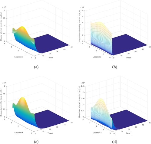
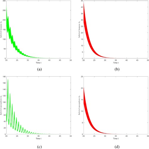
Figure 1. The evolution of infection compartments of humans and mosquitoes when and
. (a) The evolution of
. (b) Then evolution of
. (c) Then evolution of
. (d) Then evolution of
.
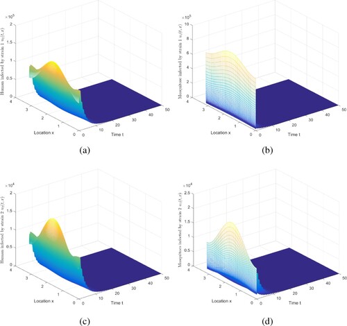
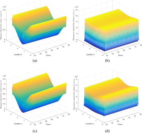
Figure 2. The evolution of infection compartments of humans and mosquitoes when and
. (a) The evolution of
. (b) The evolution of
. (c) The evolution of
. (d) The evolution of
.
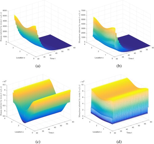
Figure 3. The evolution of infection compartments of humans and mosquitoes when and
. (a) The evolution of
. (b) Then evolution of
. (c) Then evolution of
. (d) Then evolution of
.
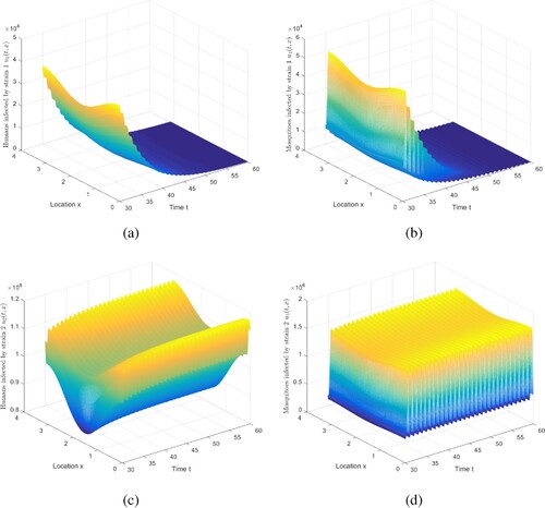
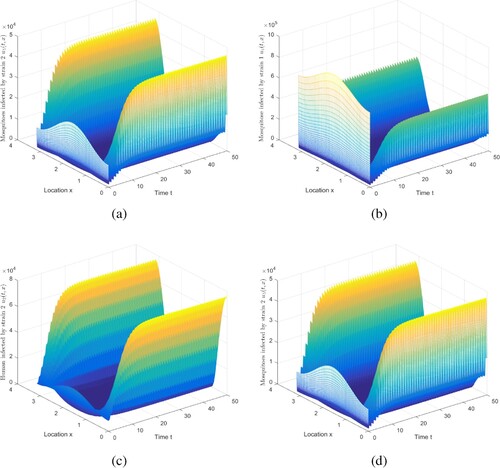
Figure 4. The evolution of infection compartments of humans and mosquitoes when and
. (a) The evolution of
. (b) The evolution of
. (c) The evolution of
. (d) The evolution of
.
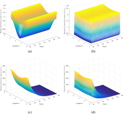
Figure 5. The evolution of infection compartments of humans and mosquitoes when and
. (a) The evolution of
. (b) The evolution of
. (c) The evolution of
. (d) The evolution of
.
6.1.1. Case 1 in Table 1
We choose ,
,
,
. Let
and
, where
,
, reflect the fact that people living in urban areas (around the centre) can enjoy added medical treatment (the number of physicians and hospitals, supply of medicines, state-of-the-art medical equipment) than people in rural area, resulting in a higher recovery rate around the centre, and maintaining the other parameters listed in Table . To compute
and
, the numerical scheme recently proposed in [Citation19, Lemma 2.5 and Remark 3.2] is used. For this set of parameters, we can numerically calculate
,
. Figure shows numerical plots of infected compartments following the initial data
Then Figure implies that two strains die out, which is coincident with Theorem 5.1. Infectious humans and mosquitoes go to 0, indicating that the disease will be eliminated under this set of parameters.
6.1.2. Case 2 and Case 3 in Table 1
Here, we simulate the result of Case 2 in Table , and then we can handle Case 3 similarly by adjusting the parameters. We choose ,
, where
,
,
,
,
,
,
,
. Figure shows that if
and
, strain 1 becomes extinct and strain 2 persists, which is consistent with Theorem 5.4. Note that we truncate the time interval by [30, 60]. Adjust the values of parameters befittingly to satisfy
and
, and the conclusion of Case 3 in Table is obtained. Details are not mentioned here.
6.1.3. Case 4 in Table 1
For Case 4 in Table , there are three results for and
. For the first conclusion, we choose
,
, where
,
,
,
,
,
, and maintain other parameters recorded in Table . Based on this set of parameters, numerically compute
and
. Figure indicates that strain 1 becomes extinct and strain 2 is persistent. Note that we truncate the time interval by [30, 60]. Because under this set of parameters, we assume that individuals and mosquitoes infected with strain 2 are more infectious and have a smaller recovery rate. Therefore, once this phenomenon occurs, there will be greater challenges to the control and eradication of malaria.
By adjusting the parameters, we can also get the result that strain 1 is persistent, and strain 2 is extinct under the condition of and
. We choose
,
, where
,
,
,
,
,
, and maintain other parameters recorded in Table . Then, compute
and
. Figure exhibits that strain 1 is persistent and strain 2 is extinct. Note that we truncate the time interval by [30, 60].
Next, the coexistence of two strains under the conditions of and
is simulated. We choose
,
, where
,
,
,
,
,
, and keep other parameters listed in Table . For this set of parameters, we can compute
and
. Figure shows that two strains can coexist, which is consistent with Theorem 5.7. Note that we truncate the time interval
to demonstrate the existence of periodic solution, in which two strains coexist.
6.2. The impact of diffusion
Except for and
, the other parameters are in accordance with in Case 1. When
and
in Case 1, then
and
, and the disease dies out. Whereas, if
and
, then
,
are exceeding 1, and the disease persists. As a consequence, the result is shown in Figure .
Figure 6. The evolution of infection compartments of humans and mosquitoes when and
. (a) The evolution of
. (b) The evolution of
. (c) The evolution of
. (d) The evolution of
.
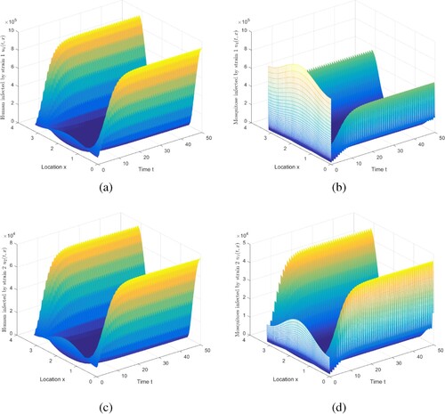
Figure shows some intriguing phenomena. In this case, malaria becomes extinct in urban areas, but persists in rural areas. It is caused by spatial heterogeneity. Because the urban environment is not apposite to mosquitoes to survive, there are relatively few mosquitoes, and there are more medical resources, the disease control in urban is relatively better. Compare with Figure , the movement will reduce disease spread risk, to a limited degree, which is consistent with the conclusion in [Citation40]. The implications include: (i) The presence of spread suggests that infected humans in rural areas can enjoy better treatment in cities. (ii) As stated in Ref. [Citation40], it is challenging for mosquitoes to collect blood meal in moving humans.
In order to understand the effect of human and mosquito movement on malaria transmission, under a set of the parameter values in Case 1, we do the following work:
(i) We assume that the diffusion coefficient of humans is , and the diffusion coefficient of mosquitoes is
(see Figure ). Trough calculation,
and
. Compared with the above
and
(Figure ), the diffusion of mosquitoes reduces the risk of disease transmission to some extent. Biologically, this may be due to the fact that there are more mosquitoes in rural areas, and infected mosquitoes move to urban areas. With the same bite rate, city has better medical conditions and a greater recovery rate, so the risk of malaria transmission will be decreased.
Figure 7. The evolution of infection compartments of humans and mosquitoes with and
. (a) The evolution of
. (b) The evolution of
. (c) The evolution of
. (d) The evolution of
.
(ii) We assume that the diffusion coefficient of humans is , but the diffusion coefficient of mosquitoes is
(see Figure ). Then
and
. Compared with the case of
and
(Figure ), humans diffusion reduces the risk of disease transmission. Biologically, it can be explained that the diffusion of humans gives them the opportunity to find a better medical environment, which will increase the recovery rate and reduce the risk of disease transmission. This may be due to the better medical conditions in the city, and the infected people will go to the city for treatment, which will increase the recovery rate and reduce the risk of disease transmission. Compared with
and
, humans diffusion has a greater impact on disease transmission. In summary, the risk of malaria transmission will be overestimated if the diffusion is ignored in the model analysis.
Figure 8. The evolution of infection compartments of humans and mosquitoes with and
. (a) The evolution of
. (b) The evolution of
. (c) The evolution of
. (d) The evolution of
.
6.3. The impact of medical resources on disease transmission
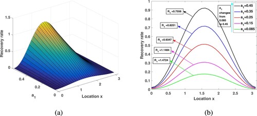
In this position, the influence of medical resources on malaria transmission is analysed from two aspects: (i) The impact of the amount of medical resources; (ii) For fixed medical resources, the influence of different allocation measures on malaria transmission. In this subsection, we take strain 1 as an example and draw conclusions about strain 2.
Since there are more medical resources in urban areas than in rural areas, people can get better medical services, and therefore have higher recovery rates. We already know that varies between
, here, take
to get the spatial distribution of the recovery rate in Figure . The corresponding medical resources in the whole region are
. In this paper, we use the recovery rate of the entire region
to represent medical resources. Choose
,
, and other parameters are consistent with those in Table . Under different medical resources, through calculation, the corresponding
is 1.4724, 1.1484, 0.9347, 0.8251, 0.7556, respectively. By observation, in a heterogeneous environment, increasing medical resources will not have a great impact on improving the recovery rate in rural areas. However, the analysis in Subsection 6.2 shows that, due to human diffusion, some patients in rural areas will go to the cities for medical treatment and enjoy better medical care, so the overall transmission risk is reduced.
Figure 9. Increasing medical resources in the environment of spatial heterogeneity and its influence on the .
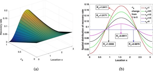
First of all, we hope to see whether maintaining a balanced distribution of urban and rural medical resources will help control the disease for a fixed recovery rate. When fixed medical resources, exploring the effect of different allocation on malaria spread. Fix and introduce a new parameter
into
, that is,
, where
, to measure the difference in medical resources allocation between urban and rural areas. As
, there is the largest gap between urban and rural medical resources, and the urban areas have the highest recovery rates. With the change of
from 1 to 0, medical resources are delivered to nearby rural areas, and the gap in medical conditions between rural and urban areas gradually is narrowed, and finally evenly distributed in space. Assume that the treatment capacity of the entire medical system is certain,
, and dose not vary with
. Select
,
, and other parameters are kept in Table . By calculation, when
takes
,
is 0.9879, 0.9911, 1.0006, 1.0171, 1.0411, respectively. Looking at Figure , the spatial heterogeneity of medical resources distribution increases the malaria spread risk, which demonstrates that the distribution of medical resources dose act a critical purpose in the pattern of malaria control. By calculation, if
, in order to make
less than 1, medical resources need at least 0.2205, but if
, the medical resources only need 0.1733, which can make
. In this way, we come to an interesting conclusion that under the condition of limited medical resources, narrowing the gap in the allocation of medical resources between rural and urban areas can better reduce the risk of malaria transmission.
Figure 10. For fixed medical resources, the spatial distribution of and the corresponding value of
.
6.4. The impact of seasonal changes in temperature and vector-bias on disease transmission
Here, we are interested in the impact of temperature-dependent EIP and vector-bias on the spread of disease. Now take single-strain subsystem (Equation10(10)
(10) ) as an example.
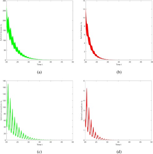
6.4.1. The role of vector-bias
To understand the influence of vector-bias on the size of malaria transmission, we make two comparison figures. The parameter value is consistent with the parameter value of Case 1, in this case, p = 0.8 and l = 0.6, i.e. , Figure (a,c), show the evolutions of infected mosquitoes and individuals at each position in
as time evolves. Adjust the values of p = 0.8 and l = 0.8, so that
, that is, there is no vector-bias effect, shown in Figure (b,d). Through observation and comparison, if vector-bias effect is not taken into account, the duration of disease extinction will be shortened, i.e. if there is no vector-bias effect, the risk of malaria transmission will be underestimated.
Figure 11. The evolution of infection compartments of humans and mosquitoes with different vector-bias parameter. Among them, green indicates that there is a vector-bias effect (), and red indicates that there is no vector-bias effect (
). (a) With vector-bias effect. (b) Without vector-bias effect. (c) With vector-bias effect. (d) Without vector-bias effect.
6.4.2. The impact of seasonal changes in temperature on disease transmission
To understand the influence of temperature-dependent EIP on malaria transmission, two comparative figures of evolution of infectious humans and mosquitoes are produced, ,
,
. The parameters are constant, that is, they are not affected by temperature, and the other parameter values are consistent with Case 1.
Figure reveals that if we do not consider seasonal changes in temperature when analysing the spread of malaria, the duration of disease extinction will be shortened, that is, the risk of disease transmission will be underestimated. This will lead to deviations in the prevention and control departments when formulating measures to control and eliminate malaria.
Figure 12. The evolution infection compartments of humans and mosquitoes with seasonal temperature changes and without seasonal temperature changes. Among them, red indicates that the parameters depend on temperature, and green indicates that the parameters do not depend on temperature.
7. Discussion
This paper proposes and analyses a reaction–diffusion malaria model with vector-bias effect and multi-strains in a periodic environment. With the purpose of exploring the dynamics, we first use the existing theory to derive ,
, and then introduce
(
). Using the comparison arguments and persistence theory of periodic semi-flow, we prove that malaria disease will be eliminated if
and
, and the strain i is extinct and the strain j is persistent if
(
). When
and
, there are three cases: (i) strain 1 is die out and strain 2 persists; (ii) strain 1 is persistent and strain 2 is extinct; (iii) the two strains coexist under the condition of
,
and exhibit spatial and seasonal fluctuations. This phenomenon is consistent with the multi-strain coexistence problem considered in Ref. [Citation30,Citation46], but they do not consider the periodic delay. Wu and Zhao [Citation40] propose a reaction–diffusion model of vector-borne disease with periodic delays to investigate the multiple effects of the temperature sensitivity of incubation periods, spatial heterogeneity, and the seasonality on disease transmission. However, they did not consider the case of multiple strains.
The numerical analysis is divided into four parts. First, the simulation results support the theoretical analysis. Second, the impact of diffusion on malaria transmission in a heterogeneous space is explored. Biologically, we figure out this spatial heterogeneity to be the difference between rural and urban regions. Simulation results show that under the condition of uneven distribution of medical resources, ignoring the diffusion of humans and mosquitoes, the risk of malaria transmission will be overestimated, which is consistent with the result in Ref. [Citation40,Citation47]. The implications include: (i) Infected humans in rural areas can seek better treatment in cities. (ii) it is challenging for mosquitoes to pick up a blood meal with moving humans. (iii) The impact of medical resources allocation on the spread of malaria is explored from two aspects: (a) increasing medical resources; (b) fixed medical resources, different allocation measures. Third, through research, we see that in the case of uneven distribution of medical resources, increasing medical resources has little impact on the spread of disease in rural areas, but it will reduce the risk of disease transmission in the entire region. Besides, when medical resources is limited, reducing the gap in the allocation of medical resources between rural and urban areas can further decrease the malaria spread risk, which is consistent with the result in Ref. [Citation40]. Therefore, when formulating measures to eliminate malaria, attention should be paid to the input of rural medical resources. Numerical results indicate that the risk of malaria may be underestimated if ignoring vector-bias effect or season. [Citation1] established a single strain ordinary differential equation model to study the effect of vector-bias on malaria transmission. The result taken by Abboubakar et al. [Citation1] in Figure shows that increasing vector-bias parameter decreases the equilibrium prevalence of infectious humans which is consistent with our conclusion.
In our study, there are some shortcomings that need to be improved. In the process of theoretical analysis, due to the complexity of periodic delays, we have not discussed all situations clearly. We have not solved the global stability of the positive periodic solution of this model. In malaria transmission model, few researchers have studied the influence of infection age and spatial diffusion on disease transmission. In fact, after malaria infection, the intensity of infectivity varies at different stages of infection. The time after infection is called the age of infection, affects the number of secondary infections. This important factor needs to be considered in the process of malaria transmission. These problems are very important for exploring the law of malaria transmission and formulating control measures. In future work, we hope to better explore them.
Acknowledgments
The authors are grateful for the support and useful comments provided by Professor Xiaoqiang Zhao (Memorial University of Newfoundland).
Disclosure statement
No potential conflict of interest was reported by the author(s).
Additional information
Funding
References
- H. Abboubakar, B. Buonomo, and N. Chitnis, Modelling the effects of malaria infection on mosquito biting behaviour and attractiveness of humans, Ric. Mat. 65(1) (2016), pp. 329–346.
- Z. Bai, R. Peng, and X.-Q. Zhao, A reaction–diffusion malaria model with seasonality and incubation period, J. Math. Biol. 77 (2018), pp. 201–228.
- H.J. Bremermann and H.R. Thieme, A competitive exclusion principle for pathogen virulence, J. Math. Biol. 27 (1989), pp. 179–190.
- R.S. Cantrell and C. Cosner, Spatial Ecology via Reaction–Diffusion Equations, John Wiley and Sons Ltd, Chichester, England, 2003.
- F. Chamchod and N.F. Britton, Analysis of a vector-bias model on malaria transmission, Bull. Math. Biol. 73(3) (2011), pp. 639–657.
- N. Chitnis, J.M. Hyman, and J.M. Cushing, Determining important parameters in the spread of malaria through the sensitivity analysis of a mathematical model, Bull. Math. Biol. 70(5) (2008), pp. 1272–1296.
- A.T. Ciota, A.C. Matacchiero, A.M. Kilpatrick, and L.D. Kramer, The effect of temperature on life history traits of Culex mosquitoes, J. Med. Entomol. 51(1) (2014), pp. 55–62.
- O. Diekmann, J.A.P. Heesterbeek, and J.A.J. Metz, On the definition and the computation of the basic reproduction ratio R0 in models for infectious-diseases in heterogeneous populations, J. Math. Biol. 28(4) (1990), pp. 365–382.
- D.A. Ewing, C.A. Cobbold, B.V. Purse, M.A. Nunn, and S.M. White, Modelling the effect of temperature on the seasonal population dynamics of temperate mosquitoes, J. Theor. Biol. 400 (2016), pp. 65–79.
- Z. Feng, Z. Qiu, Z. Sang, C. Lorenzo, and J. Glasser, Modeling the synergy between HSV-2 and HIV and potential impact of HSV-2 therapy, Math. Biosci. 245(2) (2013), pp. 171–187.
- J. Ge, K.I. Kim, Z. Lin, and H. Zhu, A SIS reaction–diffusion-advection model in a low-risk and high-risk domain, J. Differ. Equ. 259 (2013), pp. 5486–5509.
- M.A. Gregson, Communicable disease control in emergencies: a field manual, Ann. Internal Med. 146(7) (2007), pp. 544–544.
- T.J. Hagenaars, C.A. Donnelly, and N.M. Ferguson, Spatial heterogeneity and the persistence of infectious diseases, J. Theor. Biol. 229(3) (2004), pp. 349–359.
- P. Hess, Periodic-Parabolic Boundary Value Problems and Positivity, Longman Scientific and Technical, Harlow, UK, 1991.
- Y. Jin and X.-Q. Zhao, Spatial dynamics of a nonlocal periodic reaction–diffusion model with stage structure, SIAM J. Math. Anal. 40(6) (2009), pp. 2496–2516.
- P. Koch-Mesina and D. Daners, Abstract Evolution Equations, Periodic Problems and Applications, Longman Scientific and Technical, Harlow, UK, 1992.
- M. Kot, Elements of Mathematical Ecology, Cambridge University Press, Cambridge, UK, 2001.
- R. Lacroix, W. R Mukabana, L. C. Gouagna, J. C Koella, and T. Smith, Malaria infection increases attractiveness of humans to mosquitoes, PLoS Biol. 3(9) (2005), Article ID e298.
- X. Liang, L. Zhang, and X.-Q. Zhao, Basic reproduction ratios for periodic abstract functional differential equations (with application to a spatial model for Lyme disease), J. Dyn. Differ. Equ. 31 (2019), pp. 1247–1278.
- X. Liu, Y. Wang, and X.-Q. Zhao, Dynamics of a climate-based periodic Chikungunya model with incubation period, Appl. Math. Model. 80 (2020), pp. 151–168.
- Y. Lou and X.-Q. Zhao, A reaction–diffusion malaria model with incubation period in the vector population, J. Math. Biol. 62(4) (2011), pp. 543–568.
- Y. Lou and X.-Q. Zhao, A theoretical approach to understanding population dynamics with seasonal developmental durations, J. Nonlinear Sci. 27 (2017), pp. 573–603.
- G. Macdonald, The analysis of equilibrium in malaria, Trop. Dis. Bull. 49(9) (1952), pp. 813–829.
- P. Magal and X.-Q. Zhao, Global attractors and steady states for uniformly persistent dynamical systems, SIAM J. Math. Anal. 37(1) (2005), pp. 251–275.
- R.H. Martin and H.L. Smith, Abstract functional differential equations and reaction–diffusion systems, Trans. Am. Math. Soc. 321(1) (1990), pp. 1–44.
- E.T. Ngarakana-Gwasira, C.P. Bhunu, and E. Mashonjowa, Assessing the impact of temperature on malaria transmission dynamics, Afr. Mat. 25(4) (2014), pp. 1095–1112.
- R.M. Nisbet and W.S.C. Gurney, The systematic formulation of population models for insects with dynamically varying instar duration, Theor. Popul. Biol. 23(1) (1983), pp. 114–135.
- R. Ross, The Prevention of Malaria, John Murray, London, 1911.
- S. Ruan, D. Xiao, and J.C. Beier, On the delayed Ross–Macdonald model for malaria transmission, Bull. Math. Biol. 70(4) (2008), pp. 1098–1114.
- Y. Shi and H. Zhao, Analysis of a two-strain malaria transmission model with spatial heterogeneity and vector-bias, J. Math. Biol. 82(4) (2021), pp. 1-42.
- H.L. Smith, Monotone Dynamical Systems: An Introduction to the Theory of Competitive and Cooperative Systems, American Mathematical Society, Providence, 1995.
- W.J. Tabachnick, Challenges in predicting climate and environmental effects on vector-borne disease episystems in a changing world, J. Exp. Biol. 213 (2010), pp. 946–954.
- H.R. Thieme, Spectral bound and reproduction number for infinite-dimensional population structure and time heterogeneity, SIAM J. Appl. Math. 70 (2009), pp. 188–211.
- C. Vargas-De-León, Global analysis of a delayed vector-bias model for malaria transmission with incubation period in mosquitoes, Math. Biosci. Eng. 9(1) (2011), pp. 165–174.
- X. Wang and X.-Q. Zhao, A malaria transmission model with temperature-dependent incubation period, Bull. Math. Biol. 79 (2017), pp. 1155–1182.
- X. Wang and X.-Q. Zhao, A periodic vector-bias malaria model with incubation period, SIAM J. Appl. Math. 77(1) (2017), pp. 181–201.
- WHO, Available at: Malaria, http://www.who.int/ith/ith_country_list.pdf
- WHO, (2018). Availabl at: World Malaria Report, https://www.who.int/malaria/media/world-malaria-report-2018/zh/
- J. Wu, Theory and Applications of Partial Functional Differential Equations, Springer, New York, 1996.
- R. Wu and X.-Q. Zhao, A reaction–diffusion model of vector-borne disease with periodic delays, J. Nonlinear Sci. 29 (2019), pp. 29–64.
- Y. Xiao and X. Zou, Transmission dynamics for vector-borne diseases in a patchy environment, J. Math. Biol. 69(1) (2014), pp. 113–146.
- D. Xu and X.-Q. Zhao, Dynamics in a periodic competitive model with stage structure, J. Math. Anal. Appl. 311 (2005), pp. 417–438.
- L. Zhang, Z. Wang, and X.-Q. Zhao, Threshold dynamics of a time periodic reaction–diffusion epidemic model with latent periodic, J. Differ. Equ. 258(9) (2015), pp. 3011–3036.
- X.-Q. Zhao, Basic reproduction ratios for periodic compartmental models with time delay, J. Dyn. Differ. Equ. 29 (2017), pp. 67–82.
- X.-Q. Zhao, Dynamical Systems in Population Biology, Springer-Verlag, London, 2017.
- L. Zhao, Z.-C. Wang, and S. Ruan, Dynamics of a time-periodic two-strain SIS epidemic model with diffusion and latent period, Nonlinear Anal.: Real World Appl. 51 (2020), Article ID 102966.
- H. Zhao, Y. Shi, and X. Zhang, Dynamic analysis of a malaria reaction–diffusion model with periodic delays and vector bias, Math. Biosci. Eng. 19(3) (2022), pp. 2538–2574.
- T. Zheng, L.-F. Nie, Z. Teng, and Y. Luo, Competitive exclusion in a multi-strain malaria transmission model with incubation period, Chaos Solitons Fractals 131 (2020), Article ID 109545.
Appendices
Appendix 1. Derivation of (i = 1, 2)
Once again, is the number of female mosquitoes of development level infection
at time t and location x. If we consider the rate of change of the number of female mosquitoes in a given development level of infection interval
, we may write
or
where
represents the rate of the population change per unit level of infection development,
denotes the positive (left to right) ‘flux’ of individuals at the level of infection development q, time t and position x, and
is the diffusive flux.
is the vector element of surface. Dividing by
gives us
Use Gauss's divergence theorem to transform the third integral into a volume integral to simplify this equation,
Taking the limit as
approaches zero produces a conservation law for the density of individuals
(A1)
(A1) This causes Equation (EquationA1
(A1)
(A1) ) reducing to
Since it is for arbitrary Ω, this integral is zero, then
(A2)
(A2) For more clarity, the form of
needs to be discussed. According to Ref. [Citation17],
depends on the independent variables, the level of infection development, time and space. However, this is usually achieved through the dependent variable, population density. Here, let
. According to Fick's law and the hypothesis of the mosquito diffusion coefficient
, write the diffusive flux as
General balance Equation (EquationA2
(A2)
(A2) ) now reduces to
(A3)
(A3) where
is the Laplacian, i.e.
. So (EquationA3
(A3)
(A3) ) can write as
(A4)
(A4) To progress any more, we must say something about the flux of mosquitoes
. This is not a flux in space but a development level of infection. All mosquito infection levels develop, and then
Write Equation (EquationA4
(A4)
(A4) ) as
(A5)
(A5) Then by the same arguments as in Ref. [Citation40] and Ref. [Citation17], we can derive the expression of
(i = 1, 2) as
is the Green function associated with
, for
and
, subject to the Neumann boundary condition.
Appendix 2.
Proof of Lemma 4.5
Proof.
Similar to the proof of Lemma 4.4, on interval ,
, one can easily obtain that
,
for all
. Choose a large number
, where
,
and
, such that for each
,
is increasing in
, and
is increasing in
. Then, both
and
satisfy the followingsystem
Thus, for a given
, one has
(A6)
(A6) where
are the evolution operators associated with
and
subject to the Neumann boundary condition, respectively. Since
is increasing in
, it easily follows that
. We assume that
. Then there exists an
such that
. According to the second equation of (EquationA6
(A6)
(A6) ), we have
for all
. Note that if
, then
. It is easy to know that
for all
from the first equation of (EquationA6
(A6)
(A6) ). This shows that
for all
, therefore, the solution map
is strongly positive whenever
.
Appendix 3.
Proof of Theorem 5.2
Proof.
(a) In this case of , it follows from Lemmas 4.2 and 4.6 that
, and therefore
. Discuss the following system with parameter
(A7)
(A7) Denote
to be the unique solution of system (EquationA7
(A7)
(A7) ) for any
, with
for all
,
, where
Let
be the Poincaré map of system (EquationA7
(A7)
(A7) ), i.e.
,
, and make
to be the spectral radius of
. From the continuity of the principle eigenvalue about parameters, we know that
. Allow
to be small enough, one has
. Based on Lemma 4.7, there exists a positive ω-periodic function
such that
is a solution of system (EquationA7
(A7)
(A7) ), where
. For
fixed above, by the global attractivity of
of system (Equation12
(12)
(12) ) and the comparison principle, there must be an integer
large enough such that
and
Thus, as
, one has
(A8)
(A8) There exists some
, for any designated
, such that
Using (EquationA7
(A7)
(A7) ), (EquationA8
(A8)
(A8) ) and the comparison theorem for abstract functional differential equation [Citation25, Proposition 1], we get
Accordingly,
uniformly for
.
Using the theory of internal chain transitive sets [Citation45, Section 1.2], for ,
uniformly, where
is a globally attractive solution of system (Equation12
(12)
(12) ). Based on the above argument, it is easy to see that
meets a nonautonomous system, which is asymptotic to the periodic system (Equation12
(12)
(12) ).
Clearly, and D are solution map and Poincaré map associated with system (Equation10
(10)
(10) ) on
, respectively. Let
be the omega limit set of
for D. Since
and
uniformly for
, one has
. Here,
represents a function which is identical to 0, i.e.
,
. Following Lemma 5.2, one has
.
For any , let
be the solution of (Equation12
(12)
(12) ) with initial data
. A solution semi-flow of (Equation12
(12)
(12) ) on
described as
Set
. Following [Citation45, Lemma 1.2.1],
is an internal chain transitive set for D, and hence
is an internal chain transitive set for
. Define
by
for
. Due to
and
being globally attractive in
, we know
, where
is the stable set of
. By [Citation45, Theorem 1.2.1], one has
, which leads to
, thence,
(b) As
, Lemmas 4.2 and 4.6 indicate
, consequently,
. Let
and
For any
, Lemma 5.2 reveals that
and
,
,
. Thus knowing
,
. Lemma 5.1 evidences that
has a strong global attractor in
.
Set
and
to be the omega limit set of the orbit
. Denote
. Next, we prove that Q cannot form a cycle for D in
.
Claim 1. For any , the omega limit set
.
For any designated ,
,
. Then, either
or
, for each
. Furthermore, by contradiction and Lemma 5.2, it is obvious that for each
, either
or
. If
for all
, then Lemma 4.1 guarantees
uniformly for
. Thereby, the
equation in (Equation10
(10)
(10) ) meets
(A9)
(A9) where
. By the comparison principle, we have
uniformly for
. Suppose that
for some
, in the light of Lemma 5.2, we obtain
,
. Accordingly,
,
. From the
equation in (Equation10
(10)
(10) ), one has
uniformly for
. Consequently, the
equation in (Equation10
(10)
(10) ) abides by a nonautonomous system, which is asymptomatic to the periodic system (Equation12
(12)
(12) ). The theory of asymptomatically periodic system [Citation45, Section 3.2] implies that
uniformly for
. Therefore,
for any
, and Q cannot form a cycle for D in
.
Consider the following time-periodic parabolic system with parameter
(A10)
(A10) For any
, set
to be the unique solution of system (EquationA10
(A10)
(A10) ) with
for all
,
, where
Let
be the Poincaré map of system (EquationA10
(A10)
(A10) ), i.e.
,
. Make
to be the spectral radius of
. Since
, choose a sufficiently small
such that
For the above fixed
, according to the continuous dependence of the solution on the initial data, there must be a constant
such that for all
with
, which leads to
for all
. We now prove the following claim.
Claim 2. For any ,
.
Assuming contradictions, for some , one has
. So there is
such that
for all
. For each
, setting
with
and
, one has
(A11)
(A11) Following (EquationA11
(A11)
(A11) ) and Lemma 5.2, we can receive
for each
, and
. Thus, as
,
and
satisfy
(A12)
(A12) Based on
for all t>0 and
, there must be a constant
such that
where
is a positive ω-periodic function such that
is a solution of system (EquationA10
(A10)
(A10) ), and
. It follows from (EquationA12
(A12)
(A12) ) and the comparison theorem that
Obviously,
as
, i = 1, 3, which leads to a contradiction.
With the above claim, it is easy to obtain that Q is an isolated invariant set for D in , and
, where
is the stable set of Q for D. For any integer n with
,
is compact, it follows that D is compact, then D is asymptotically smooth on
. Moreover, by Lemma 5.1, we obtain that D has a global attractor on
. According to [Citation24, Theorem 3.7], D has a global attractor
in
. Based on the acyclicity theorem on uniform persistence for maps [Citation45, Theorem 1.3.1, Remark 1.3.1], then D is uniformly persistent with respect to
in the sense that there exists an
, such that
(A13)
(A13) Now we derive the practical persistence required. Following
, then
and
for any
. Set
. Obviously,
and
,
. Define a continuous function
by
Because
is a compact subset of
, we obtain that
. Consequently, there is an
such that
Furthermore, according to Lemma 5.2, there must be an
such that
The existence of a positive periodic steady state remains to be proved. By [Citation2, Lemma 8] and [Citation45, Theorem 3.5.1], for each t>0, the solution map
of system (Equation10
(10)
(10) ), is a κ-contraction with respect to an equivalent norm on
, where κ is Kuratowski measure of noncompactness. Define
and
For any
,
is
-uniformly persistent with
is easily attainable. It then follows from [Citation24, Theorem 4.5], as applied to
, that system (Equation10
(10)
(10) ) has an ω-periodic solution
with
. Let
,
and
, where
. Combing the uniqueness of solutions and Lemma 5.2, we have that
is periodic solution of system (Equation10
(10)
(10) ), and it is also strictly positive.
Appendix 4.
Proof of Lemma 5.2
Proof.
According to the comparison principle for cooperative systems, we have , and
for all t>0 and
. Moreover,
and
satisfy
where
,
,
are defined in Section 3. If there exists
, such that
and
, one has
and
,
, based on the strong maximum principle [Citation14, Proposition 13.1]. Set
to be the solution of
(A14)
(A14) Clearly,
is Hölder continuous and nonnegative nontrivial on
. By the comparison principle,
In addition, from [Citation43, Lemma 2.1], system (EquationA14
(A14)
(A14) ) admits a unique positive ω-periodic
, which is globally attractive. Then
uniformly for
. The proof is complete.
Appendix 5.
Parameter definition and value
Wang et al. [Citation36] have studied the seasonal factors that affect malaria transmission, including seasonal forced bite rate
(A15)
(A15) periodic mortality rate of mosquitoes
(A16)
(A16) periodic EIP
(A17)
(A17)
(A18)
(A18) and mosquitoes recruitment rate
(A19)
(A19) In addition, due to the assumption of vector-bias effect, and according to Ref. [Citation35], in the following simulations, we take p = 0.8 and l = 0.6.
In order to better understand the periodicity and biological significance of the above parameters, we make the following figures. Looking at Figure , the distribution and seasonal dynamics of mosquito populations are affected by climate change. Analysing Figure (a), the peak of mosquito bites happens during warm or rainy seasons (May to September). In a year, the death rate may be lower in spring and summer when the humidity and temperature are suitable for species growth, and higher in winter due to low temperature and dry weather. In addition, higher temperature can shorten the duration of EIP.
Figure A1. A small interval of development level of infection.
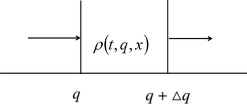
Figure A2. The parameters change with time. (a) Change of contact rate with time. (b) Change of EIP
with time. (c) Change of the death rate of mosquitoes
with time.
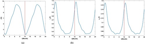
Table F1. Definition and value of parameters.