Optimal reduced-mixing for an SIS infectious-disease model

Abstract

Which reduced-mixing strategy maximizes economic output during a disease outbreak? To answer this question, we formulate an optimal-control problem that maximizes the difference between revenue, due to healthy individuals, and medical costs, associated with infective individuals, for SIS disease dynamics. The control variable is the level of mixing in the population, which influences both revenue and the spread of the disease. Using Pontryagin's maximum principle, we find a closed-form solution for our problem. We explore an example of our problem with parameters for the transmission of Staphylococcus aureus in dairy cows, and we perform sensitivity analyses to determine how model parameters affect optimal strategies. We find that less mixing is preferable when the transmission rate is high, the per-capita recovery rate is low, or when the revenue parameter is much smaller than the cost parameter.

Keywords:

• Optimal control
• infectious-disease modeling
• bovine mastitis
• social distancing

1. Introduction

Infectious-disease outbreaks are a growing problem. The rate at which diseases emerge or re-emerge is increasing [15,31,48,60,62] due to factors such as global travel, rural-to-urban migration, and climate change [2,4,62,64]. Examples of recent disease outbreaks include foot and mouth disease [37], African swine fever [19], olive quick decline syndrome [53], tomato brown rugose fruit virus [67], tuberculosis [45], Zika [43], SARS [17], swine flu or H1N1 [41], Ebola [33], and COVID-19 [17]. Many of these diseases have had severe economic consequences [5,36,37,53,61]. We clearly need to know how to respond to new outbreaks if and when they occur.

Ideally, we would like to minimize the duration of an outbreak, the cost of illness, or the cost of mitigation strategies. We may also wish to optimize some combination of these often-conflicting objectives. To achieve these goals, researchers often use optimal control theory to efficiently control dynamic disease systems [11,22,46,56–58,65]. In general, these systems consist of state variables, control variables, and state equations. The state variables often represent disease classes within a population, such as the number of susceptible (S), infective (I), or recovered (R) individuals, as functions of time. The control variables and the state equations govern the evolution of the state variables, and we want to choose the control variables so as to maximize or minimize specified objective functionals [38].

An especially important topic in the study of emerging infectious diseases is the use of optimal control theory to control mixing. The goal here is to design strategies that limit the number of contacts between susceptible and infectious individuals. For humans, strategies may include social-distancing measures such as limiting time spent in public spaces, isolating infectives, quarantining infected households, closing schools, and restricting large social gatherings [3,51,52]. For livestock, reduced-mixing strategies may include quarantining infected and exposed animals and shutting down facilities where animals are in close contact. For crops, reduced-mixing strategies may include using screenhouses, introducing barrier plants, or reducing planting density [16,29,32]. Many of these strategies do, however, have high economic costs [21,25,26,30,40,50].

To address these economic costs, many researchers have tried to balance economic output with the cost of infection, which can include death or the burden of disease on an individual or on medical and public health infrastructures. These researchers have frequently used complex multi-compartmental models, which they solve numerically, to minimize the size of an outbreak [6] or to minimize both the size and economic cost of an outbreak [8,39,58,59].

In this paper, we instead focus on finding simple, analytic optimal-mixing strategies for SIS disease dynamics. In an SIS model, individuals are either susceptible or infectious, and individuals who recover may then be reinfected. This model is used to study diseases that do not confer immunity after recovery, such as rotaviruses, sexually transmitted infections, and many bacterial infections [34]. Also, as noted by [14], SIS models are often appropriate for diseases that confer variant-specific immunity, such as when many variants are circulating in a population. Examples of SIS models, in practice, include models of Staphylococcus aureus in dairy cows [63], typhoid fever in humans [24], trachoma in humans [23], trypanosomiasis in Indonesian buffaloes [14], and gonorrhea in humans [12,28].

In Section 2, we introduce an optimal-control problem, with SIS disease dynamics, that will let us determine whether reduced mixing is economically beneficial. We assume that economic profit, be it for a farm or a company, is the revenue generated by healthy susceptibles minus the cost of sick infectives over the given time interval. The control variable is the level of mixing in the population, which can range from little or no mixing to high or full mixing. In particular, the ability to reduce mixing may be limited by economic constraints or by a lack of willingness to comply with guidelines, and the ability to mix may be limited by fear of spreading disease or the need to gather resources to restart production.

In Section 3, we determine closed-form optimal solutions and find that reducing mixing can improve economic output. We also study under which conditions a longer period of reduced mixing is more profitable. We find that the optimal reduced-mixing strategy is bang-bang and has at most one switch from the lowest possible level of mixing to the highest possible level of mixing.

In Section 4, we use parameters for the transmission of Staphylococcus aureus in dairy cows and compare our analytical solutions with numerical simulations. Then, in Section 5, we explore the effects of varying key parameters such as the minimum and maximum mixing levels, the revenue generated per susceptible per day, the cost per infective per day, and the time horizon. We also look at the effects of varying the infectiousness, recovery time, and the initial number of infected individuals on the optimal length of the reduced-mixing period. Finally, in Section 6, we summarize our results and discuss the limitations and future directions of our research.

2. Optimizing reduced-mixing for an SIS model

We wish to maximize economic output during an infectious-disease outbreak. In this section, we assume that our outbreak obeys SIS dynamics. The SIS model describes a population transitioning from a susceptible state to an infectious state and back [35]. These models are commonly used for studying diseases that do not confer immunity upon recovery [34].

The ordinary differential equations (ODEs) for the SIS model are (1) $\begin{array}{rl}\frac{\mathrm{d}S}{\mathrm{d}t}& =-a\left(t\right)\text{β}SI+\gamma I,\end{array}$(1) (2) $\begin{array}{rl}\frac{\mathrm{d}I}{\mathrm{d}t}& =a\left(t\right)\text{β}SI-\gamma I,\end{array}$(2) where $S\left(t\right)$ and $I\left(t\right)$ are state variables representing the number of susceptible and infectious individuals in the population. Some authors [27,34] use S and I for the fractions of a population that are susceptible or infectious. We instead follow [35] and many other authors, e.g., [9,10], in using these variables for the numbers of susceptibles and infectives.

In the above equations, the control variable $a\left(t\right)$ represents the level of mixing of the population at time t. The mixing level ranges between m, for the lowest possible level of mixing, and M, for the highest possible level of mixing. Both m and M can range between zero, for no mixing, and one, for full or normal levels of mixing. The parameter β is the transmission coefficient, or the rate of infection per susceptible per infective. The parameter γ represents the per-capita rate of recovery for infected individuals.

After adding Equations (1(1) $\begin{array}{rl}\frac{\mathrm{d}S}{\mathrm{d}t}& =-a\left(t\right)\text{β}SI+\gamma I,\end{array}$(1) ) and (2(2) $\begin{array}{rl}\frac{\mathrm{d}I}{\mathrm{d}t}& =a\left(t\right)\text{β}SI-\gamma I,\end{array}$(2) ), it quickly follows that S + I = N, where N is the total population size. We can, as a result, reduce Equations (1(1) $\begin{array}{rl}\frac{\mathrm{d}S}{\mathrm{d}t}& =-a\left(t\right)\text{β}SI+\gamma I,\end{array}$(1) ) and (2(2) $\begin{array}{rl}\frac{\mathrm{d}I}{\mathrm{d}t}& =a\left(t\right)\text{β}SI-\gamma I,\end{array}$(2) ) to a single state equation, (3) $\begin{array}{r}\frac{\mathrm{d}I}{\mathrm{d}t}=a\left(t\right)\text{β}(N-I)I-\gamma I,\end{array}$(3) with the initial condition $I\left(t\right)=I_0$, where $I_0<N$. Our state equation and control variable in this case are like those in [55]. We focus, however, on reducing general mixing rather than on solely quarantining infectives.

The objective functional that we will maximize is (4) $\underset{m\le a\left(t\right)\le M}{max}{\int }_0^{T}ra\left(t\right)[N-I(t\left)\right]-cI\left(t\right)\mathrm{d}t.$(4) The first term in the objective functional is the revenue generated by the active susceptible population, while the second term represents the cost generated by infected individuals. Higher activity increases revenue but also increases the spread of the disease.

The parameter r is the revenue generated per healthy susceptible per day, and the parameter c is the cost per sick infective per day. This cost is separate from (and in addition to) lost revenue or productivity. The parameter c typically includes medical or treatment costs. Both r and c are, by assumption, positive. T is the terminal time, also called the time horizon. It can be chosen based on factors such as vaccine development time or using economic or logistical criteria.

This formulation assumes that infective individuals do not contribute economically, but that they do interact with the population to the extent that the control variable, which limits mixing, permits. For humans, we assume, in other words, that infectives are too sick to work, but not too sick to interact with household members, health-care workers, and others. For livestock, we assume that sick animals cannot produce goods, but that they do still interact with other animals. For crops, we assume that infected plants cannot be sold but do contribute to the spread of a disease.

3. Analytical solutions

We will determine the analytical solutions to the optimal-control problem described in Section 2 using Pontryagin's maximum principle [44]. First, we need to define the control Hamiltonian, H. The Hamiltonian is (5) $\begin{array}{rl}H& =f(t,I,a)+\lambda g(t,I,a)\\ & =a\left(t\right)[N-I(t\left)\right][r+\lambda (t\left)\text{β}I\right(t\left)\right]-I\left(t\right)[c+\lambda (t\left)\gamma \right],\end{array}$(5) where $f(t,I,a)$ is the integrand of objective functional (4(4) $\underset{m\le a\left(t\right)\le M}{max}{\int }_0^{T}ra\left(t\right)[N-I(t\left)\right]-cI\left(t\right)\mathrm{d}t.$(4) ) and $g(t,I,a)$ is the right-hand side of state Equation (3(3) $\begin{array}{r}\frac{\mathrm{d}I}{\mathrm{d}t}=a\left(t\right)\text{β}(N-I)I-\gamma I,\end{array}$(3) ).

For the problem given by Equations (3(3) $\begin{array}{r}\frac{\mathrm{d}I}{\mathrm{d}t}=a\left(t\right)\text{β}(N-I)I-\gamma I,\end{array}$(3) ) and (4(4) $\underset{m\le a\left(t\right)\le M}{max}{\int }_0^{T}ra\left(t\right)[N-I(t\left)\right]-cI\left(t\right)\mathrm{d}t.$(4) ), the maximum principle tells us that, for the optimal trajectories $I^{\ast }\left(t\right)$ and $a^{\ast }\left(t\right)$, there exists a piecewise-differentiable adjoint variable, $\lambda \left(t\right)$, obeying the differential equation (6) $\begin{array}{rl}\dot{\lambda }\left(t\right)& =-\frac{\mathrm{\partial }H(t,I(t),a(t),\lambda (t\left)\right)}{\mathrm{\partial }I}\\ & =a[r-\lambda \text{β}(N-2I)]+c+\gamma \lambda \end{array}$(6) and the transversality condition $\lambda \left(T\right)=0$. The maximum principle also tells us that (7) $H(t,I^{\ast }(t),a(t),\lambda (t\left)\right)\le H(t,I^{\ast }(t),a^{\ast }(t),\lambda (t\left)\right)$(7) for all possible a at time t [7,38].

Before we find the analytical solution, it is helpful to note that we have defined an optimization problem with three variables: the state variable, $I\left(t\right)$, the control variable, $a\left(t\right)$, and the adjoint variable, $\lambda \left(t\right)$. In addition to maximization condition (7(7) $H(t,I^{\ast }(t),a(t),\lambda (t\left)\right)\le H(t,I^{\ast }(t),a^{\ast }(t),\lambda (t\left)\right)$(7) ), the problem is subject to two ODEs that describe the dynamics of the state and adjoint variables. We also have an initial condition for the state equation and a terminal condition for the adjoint equation. Therefore, the ODEs form a two-point boundary value problem. In general, we want to solve the state equation forwards in time and the adjoint equation backwards in time.

Now, we can begin to solve the problem. First, we observe that the Hamiltonian is linear in the control variable, (8) $H=a\varphi \left(t\right)-(c+\lambda \gamma )I,$(8) where (9) $\varphi =(N-I)(r+\lambda \text{β}I)$(9) is known as the switching function.

The above linearity implies that the form of the optimal control that maximizes the Hamiltonian is bang-bang. If the switching function is either positive or negative, the optimal control is (10) $\begin{array}{r}a\left(t\right)=\{\begin{array}{ll}m,& \varphi \left(t\right)<0,\\ M,& \varphi \left(t\right)>0.\end{array}\end{array}$(10) A switch occurs when $\varphi =0$ or when (11) $\lambda =-\frac{r}{\text{β}I}.$(11) In addition, cases may arise where the optimal-control model has a singular solution. This occurs if $\varphi \left(t\right)=0$ over an entire interval. To determine if a singular solution exists for our problem, we set the derivative of λ, obtained from switching condition (11(11) $\lambda =-\frac{r}{\text{β}I}.$(11) ), equal to Equation (6(6) $\begin{array}{rl}\dot{\lambda }\left(t\right)& =-\frac{\mathrm{\partial }H(t,I(t),a(t),\lambda (t\left)\right)}{\mathrm{\partial }I}\\ & =a[r-\lambda \text{β}(N-2I)]+c+\gamma \lambda \end{array}$(6) ) at the time of the switch. From this, we find that a singular solution is only possible for c = 0. Since c is positive, this precludes the possibility of a singular solution for our problem.

The next step is to solve the state and adjoint equations using what we have learned about the control. To do this, we will assume that at most one switch occurs, which we will demonstrate later. Also, the transversality condition for the adjoint equation tells us that $\lambda \left(T\right)=0$, so that $\varphi \left(T\right)=r(N-I)$ is positive, in light of Equation (3(3) $\begin{array}{r}\frac{\mathrm{d}I}{\mathrm{d}t}=a\left(t\right)\text{β}(N-I)I-\gamma I,\end{array}$(3) ) and our assumption that $I_0<N$. We now know, from Equation (10(10) $\begin{array}{r}a\left(t\right)=\{\begin{array}{ll}m,& \varphi \left(t\right)<0,\\ M,& \varphi \left(t\right)>0.\end{array}\end{array}$(10) ), that $a\left(T\right)=M$. In other words, the solution to the optimal-control problem must be at the highest level of mixing at the final time. This implies that if a switch occurs, the switch will be from the lowest level of mixing, a = m, to the highest level of mixing, a = M. If no switch occurs, the population is always at the highest level of mixing.

If we assume that at most one switch occurs, we can find an analytical solution to the generalized optimal-control model. Before the switch occurs at $t=t_1$, we know that a = m. Using this and the initial condition, $I\left(0\right)=I_0$, we solve the state equation for times $t\le t_1$ to get (12) $I\left(t\right)=\frac{{\delta }_m{I}_0}{m\text{β}{I}_0+({\delta }_m-m\text{β}{I}_0)e^{-{\delta }_{m}t}},$(12) where ${\delta }_m=mN\text{β}-\gamma$.

Similarly, we can solve the state equation at times $t\ge t_1$ using the conditions $I\left(t_1\right)=I_1$ and a = M for $t\ge t_1$. The solution to the state equation after the switch is (13) $I\left(t\right)=\frac{{\delta }_M{I}_1}{M\text{β}{I}_1+({\delta }_M-M\text{β}{I}_1)e^{-{\delta }_M(t-t_1)}},$(13) where ${\delta }_M=MN\text{β}-\gamma$. By evaluating Equation (12(12) $I\left(t\right)=\frac{{\delta }_m{I}_0}{m\text{β}{I}_0+({\delta }_m-m\text{β}{I}_0)e^{-{\delta }_{m}t}},$(12) ) at time $t_1$, we find $I_1$, which is used in Equation (13(13) $I\left(t\right)=\frac{{\delta }_M{I}_1}{M\text{β}{I}_1+({\delta }_M-M\text{β}{I}_1)e^{-{\delta }_M(t-t_1)}},$(13) ).

To solve the adjoint equation, we again find the solution in two parts. Since we have the transversality condition, $\lambda \left(T\right)=0$, we will solve the adjoint equation backwards in time. First, we will determine the solution to the adjoint equation after the switch. When $t>t_1$, we know that a = M, and the adjoint equation is (14) $\dot{\lambda }\left(t\right)+[{\delta }_M-2M\text{β}I(t\left)\right]\lambda \left(t\right)=Mr+c.$(14) Using an integrating factor and the transversality condition, we find that the solution after the switch is (15) $\lambda \left(t\right)=\frac{(Mr+c)[1-e^{{\delta }_M(T-t)}]u\left(t\right)}{{\delta }_{M}u\left(T\right)},$(15) where (16) $u\left(t\right)=({\delta }_M-M\text{β}{I}_1)+M\text{β}{I}_1{e}^{{\delta }_M(t-t_1)}.$(16) Before the switch, we know that $t<t_1$ and a = m. With this information, we can solve the adjoint equation before the switch. Using an integrating factor, and the condition that the solution must equal Equation (15(15) $\lambda \left(t\right)=\frac{(Mr+c)[1-e^{{\delta }_M(T-t)}]u\left(t\right)}{{\delta }_{M}u\left(T\right)},$(15) ) at time $t_1$, we find that the solution to the adjoint equation before the switch is (17) $\lambda \left(t\right)=\frac{e^{-{\delta }_{m}t}v\left(t\right)}{m\text{β}{I}_0{\delta }_m}[\frac{cv\left(t\right)}{v\left(t_1\right)}-(mr+c\left)\right],$(17) where (18) $v\left(t\right)=({\delta }_m-m\text{β}{I}_0)+m\text{β}{I}_0{e}^{{\delta }_{m}t}.$(18) By setting Equation (15(15) $\lambda \left(t\right)=\frac{(Mr+c)[1-e^{{\delta }_M(T-t)}]u\left(t\right)}{{\delta }_{M}u\left(T\right)},$(15) ) for the adjoint variable equal to switching condition (11(11) $\lambda =-\frac{r}{\text{β}I}.$(11) ), we find the ratio of the revenue and cost parameters as a function of the switching time, (19) $\frac{r}{c}=\frac{{\delta }_m{I}_0\text{β}[e^{{\delta }_M(T-t_1)}-1]}{{\delta }_M[m\text{β}{I}_0+({\delta }_m-m\text{β}{I}_0\left)e^{-{\delta }_m{t}_1}\right]},$(19) This allows us to numerically solve for the switching time. The effect of the ratio of the revenue and cost parameters on the switching time will be explored numerically in Section 5.1.1.

To prove that at most one switch occurs, we show that a second switch cannot occur before $t_1$. This means that we must have (20) $\lambda \left(t\right)<-\frac{r}{\text{β}I\left(t\right)}$(20) for all $t<t_1$. Plugging in solutions (17(17) $\lambda \left(t\right)=\frac{e^{-{\delta }_{m}t}v\left(t\right)}{m\text{β}{I}_0{\delta }_m}[\frac{cv\left(t\right)}{v\left(t_1\right)}-(mr+c\left)\right],$(17) ) and (12(12) $I\left(t\right)=\frac{{\delta }_m{I}_0}{m\text{β}{I}_0+({\delta }_m-m\text{β}{I}_0)e^{-{\delta }_{m}t}},$(12) ) for the adjoint and state equations before the switch at $t=t_1$, Equation (20(20) $\lambda \left(t\right)<-\frac{r}{\text{β}I\left(t\right)}$(20) ) becomes (21) $\frac{e^{-{\delta }_{m}t}v\left(t\right)}{m\text{β}{I}_0{\delta }_m}[\frac{cv\left(t\right)}{v\left(t_1\right)}-(mr+c\left)\right]<-\frac{r{e}^{-{\delta }_{m}t}v\left(t\right)}{\text{β}{\delta }_m{I}_0},$(21) which reduces to $v\left(t\right)<v\left(t_1\right)$, where $v\left(t\right)$ is defined in Equation (18(18) $v\left(t\right)=({\delta }_m-m\text{β}{I}_0)+m\text{β}{I}_0{e}^{{\delta }_{m}t}.$(18) ). Since for $0<t<t_1$ equation $v\left(t\right)<v\left(t_1\right)$ is true, we know that we can have at most one switch.

Figure 1 shows a typical ($\lambda ,I$) phase portrait, on both sides of the switching function. This figure provides further evidence that, for various terminal times, only one switch is possible.

Figure 1. Phase portrait of the optimal-control problem. The parameters used in this example are given in Table 1 with the exception of $I_0$, which we set to 499 individuals. In this figure, we see the behavior of λ, the adjoint variable (solid curves) and the value of the switching function (dashed curve) versus I, the number of infective individuals. Each of the solid lines is from an evaluation of the optimal-control model for a different terminal time. In this figure, we can see that the adjoint variable crosses the switching function at most once for each simulation. The thin solid line shows the phase portrait of the case study in Section 4.

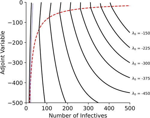
Table 1. Parameters used for numerical verification.

Parameter	Value	Meaning
β	${\displaystyle \frac{0.0232}{N}}$ (indiv·day)${}^{-1}$	Transmission coefficient
γ	$\frac{1}{110}$ day${}^{-1}$	Per-capita recovery rate
T	90 days	Time horizon
r	0.39 ${\displaystyle \frac{\mathrm{U}\mathrm{S}\mathrm{\$}}{\mathrm{i}\mathrm{n}\mathrm{d}\mathrm{i}\mathrm{v}\cdot \mathrm{d}\mathrm{a}\mathrm{y}}}$	Revenue per susceptible per day
c	6.83 ${\displaystyle \frac{\mathrm{U}\mathrm{S}\mathrm{\$}}{\mathrm{i}\mathrm{n}\mathrm{d}\mathrm{i}\mathrm{v}\cdot \mathrm{d}\mathrm{a}\mathrm{y}}}$	Cost per infective per day
m	0.2	Minimum mixing level
M	0.9	Maximum mixing level
$I_0$	0.05N individuals	Initial number of infectives
N	500 individuals	Total population size

Sources: Disease parameters are estimated from [63]. Revenue and cost parameters are estimated from [49].

A special case of the above SIS system occurs when $\gamma =0$. Now, infected individuals do not recover. In this case, our outbreak obeys a simple epidemic, or SI, model [1]. This model is frequently used to describe highly-infectious diseases that are not serious [1,18] or to study the initial (pre-recovery) stages of many other diseases [10]. The solution to the optimal-control problem for the SI case can be found by letting $\gamma =0$ in the above solutions. For example, the ratio of the revenue and the cost parameters as a function of the switching time for the SI system is now just (22) $\frac{r}{c}=\frac{[e^{MN\text{β}(T-t_1)}-1]I_0}{M[(N-I_0)e^{-mN\text{β}{t}_1}+I_0]}.$(22)

4. Case study: bovine mastitis

As an example, we consider the transmission of Staphylococcus aureus genotype B (GTB) in Swiss communal dairy herds [63]. S. aureus GTB is a contagious pathogen that commonly causes mastitis in dairy cows. Mastitis, an inflammation of the mammary gland, leads to economic loss in the dairy industry due to reduced yield and poor milk quality. Mastitis can be categorized as clinical or subclinical. In cases of clinical mastitis, abnormalities are visible and can include watery milk with flakes or clots, a red and swollen udder, or fever. In cases of subclinical mastitis, which is more prevalent, abnormalities are not visually detectable and, therefore, cases of subclinical mastitis are often undetected.

Both classes of mastitis decrease milk production during and after infection, but subclinical mastitis accounts for more financial loss than clinical mastitis due to its prevalence. This financial loss is, however, difficult to quantify [13,49]. We will, therefore, use the economics associated with clinical mastitis to determine revenue and cost parameters, while keeping in mind that clinical mastitis is more costly (than subclinical mastitis) on a per-case basis.

In this example, revenue comes from milk produced by the dairy cows, and cost includes the cost of veterinary care, diagnostics, labor, therapeutics, future production loss, and future reproductive loss. These parameters were estimated from [49]. It is important to note that if infected cows are treated with antibiotics during the lactation period, the milk produced is discarded due to contamination. The treatment of subclinical mastitis with antibiotics is not generally cost effective. For highly contagious pathogens like S. aureus, however, treatment is still recommended [47]. Reduced-mixing strategies are also useful for preventing the spread of S. aureus and include quarantining cows with mastitis and milking cows with mastitis on separate machines or after uninfected cows [66].

As subclinical mastitis cases often go undetected, it may be beneficial to treat cows that are more likely to have subclinical mastitis, such as those with higher somatic cell counts (SCC), as infected. Thus, when the level of mixing is low, more cows are quarantined or milked separately. We also assume that they are treated with antibiotics. Treatment costs and costs due to future production loss are only applied to infectives as we are assuming a higher cost of treatment associated with clinical mastitis, and only infectives will have future production losses.

We use a time horizon of 90 days because the communal pasture-based dairy operations, in our example, occur in the 2 to 3 months of the summer when cows are brought together at higher altitudes where they share pastures, milking equipment, and housing facilities. As the mean duration for intramammary infections is 110 days, an outbreak during this time can be significant [63]. We adapted the transmission coefficient and the per-capita recovery rate for our simulation of mastitis from [63]. In their model, the transmission coefficient is estimated as $\text{β}N=0.0232$ per day, so to adapt their parameter to our model, we divide by N. In [63], transmission is assumed to be cow-to-cow. Also, S represents susceptible cows, and I represents infected cows.

The parameters used to model the dynamics of S. aureus GTB transmission are in Table 1. The values of the parameters m and M are unknown, so we assume the values m = 0.2 and M = 0.9. We assume m = 0.2 as the minimum mixing level as it is unlikely that mixing between dairy cows can be completely eliminated due to spatial limitations at housing facilities and human error in milking practices that may lead to exposure to pathogens. We assume M = 0.9 as recommended milking practices will reduce mixing to some extent. We will see how different choices for m and M affect the results of our problem in Section 5.1.2.

To numerically solve our optimal-control problem we chose to explore freely available, optimal-control toolkits, including the dsoa package [20]. From the available options, we found dsoa to be the easiest to implement, and it was able to converge for all tested cases. This package transforms the optimal-control problem into a nonlinear programming problem that can be solved using sequential quadratic programming.

Figure 2 shows that with the parameter values for S. aureus GTB transmission given in Table 1 and the SIS state equations, the results from using dsoa and the analytical solutions are the same. In this case, the optimal solution is to switch to a higher level of mixing about halfway through the simulation. At the time of the switch, which is after 44 days, about 4% of the population is infected, and, at the terminal time, about 6% of the population is infected. These dynamics are reasonable, because subclinical mastitis is a mild infection. Thus, when low levels of infection are present, the cost of care and loss of productivity are not too high.

Figure 2. Analytical results and numerical results for the general SIS model. This figure shows that for the parameters given in Table 1, the results from using dsoa and the analytical solutions are the same. Figure (A) shows that the activity level, a, switches after about 44 days. Figure (B) shows that the infective population, I, decreases before the switch, and then increases after the switch.

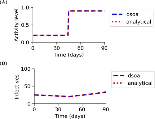
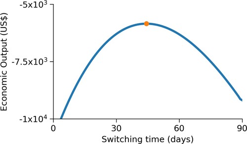
Figure 3 shows that the switching time determined in this solution maximized the economic output relative to other possible switching times.

Figure 3. Verification of results for the optimal switching time. For the parameters given in Table 1, we vary $t_1$ from 0 days to T days and calculate the value of the objective functional. The solution for optimal switching time is shown as the dot. For the general SIS model, the maximum economic output is achieved at the solution for the optimal switching time, at about 44 days.

5. Sensitivity of results to model parameters

In Section 5.1.1, we will determine how changes in the ratio of the revenue and cost parameters change the switching time from that of the baseline simulations. We will see that, for the SIS model, reducing mixing is economically beneficial in many cases. In Section 5.1.2, we will vary the minimum and maximum mixing levels for the population and find that increasing either increases the switching time. In Section 5.1.3, we will vary the terminal time, T, and find that the switching time increases with the time horizon. In Section 5.2, we will vary the transmission coefficient as well as the per-capita recovery rate to see how the implementation of mitigation strategies affects the switching time. We also vary $I_0$ to determine how the initial number of infectives affects the optimal switching time. In all of Section 5, we use analytic formula (19(19) $\frac{r}{c}=\frac{{\delta }_m{I}_0\text{β}[e^{{\delta }_M(T-t_1)}-1]}{{\delta }_M[m\text{β}{I}_0+({\delta }_m-m\text{β}{I}_0\left)e^{-{\delta }_m{t}_1}\right]},$(19) ) for the ratio of the revenue and cost parameters from the SIS model to determine how switching times vary with model parameters. In Figure 4, we verify these results numerically using dsoa.

Figure 4. Switching time as a function of the ratio of the revenue and cost parameters. In this figure, we see that the switching time decreases as the revenue parameter increases relative to the cost parameter. This plot is for the SIS model with the parameters given in Table 1. In this example, the optimal mixing strategy greatly depends on the value of the revenue parameter. The solid curve corresponds to Equation (19(19) $\frac{r}{c}=\frac{{\delta }_m{I}_0\text{β}[e^{{\delta }_M(T-t_1)}-1]}{{\delta }_M[m\text{β}{I}_0+({\delta }_m-m\text{β}{I}_0\left)e^{-{\delta }_m{t}_1}\right]},$(19) ) while the circles are points where the switching time was computed numerically, using dsoa.

5.1. Sensitivity with respect to optimal-control parameters

First, we would like to see how changes in optimal-control parameter values affect the optimal switching time. If these changes are significant, it indicates that correctly estimating the revenue and cost parameters, minimum and maximum mixing levels, and the time horizon not only adds to our understanding of the disease but is also important for determining the best reduced-mixing strategy.

5.1.1. Effects of varying the revenue and cost parameters

One of the most important components of our model is the switching time, or when the population should change from a lower mixing level to a higher mixing level. Since we want to explore the optimal switching time from an economic perspective, we first look at how the ratio of the revenue and cost parameters affects the switch.

The effect of the ratio of the revenue and cost parameters on the switching time when the SIS model is used can be seen in Figure 4. We can see that as the revenue parameter, r, increases relative to the cost parameter, c, the switching time decreases. When r is much smaller than c, the switch happens later. When r is approximately 0.2 times c, a switch no longer occurs and the population remains at the higher mixing level the entire time. This tells us that, for a mild illness like in our example, mixing should be reduced only if the cost associated with a sick infective is significantly greater than the potential revenue.

5.1.2. Effects of varying M and m

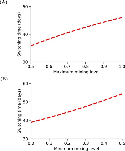
For the SIS model, we defined m to be the minimum mixing level and M to be the maximum mixing level. The values of these parameters limit the intensity of the reduced-mixing strategy. Figure 5 shows us that increasing M causes an increase in the switching time. This increase is about 10 days. We also see that increasing m increases the switching time. In this example, there is a greater difference of about 15 days as m increases. Therefore, changes in the lowest and highest possible levels of mixing could result in a significant difference in the amount of time spent at the lowest level of mixing.

Figure 5. Changes in switching time, $t_1$, due to changes in activity levels. In (A), we increase the maximum mixing level, M, from 0.5 to 1 while holding m = 0.2 constant, and in

(B), we increase the minimum mixing level, m, from 0.01 to 0.5 while holding M = 0.9 constant. In both cases, we see that the switching time increases as the highest or lowest possible level of mixing increases.

5.1.3. Effects of varying T

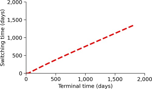
The last optimal-control parameter we vary is T, the time horizon of the simulation. This parameter is an important component of the model and can represent the time for a vaccine to be developed, the time for an infectious disease to run through the population, or a fiscal quarter or year. For our example, T was determined by the amount of time that communal pasture-based dairy operations are typically used. We can see, in Figure 6, the switching time increases monotonically with the terminal time.

Figure 6. Changes in switching time, $t_1$, due to changes in the time horizon. This figure shows how the switching time changes depending on the terminal time of the simulation, T. We see that as the terminal time increases, the switching time also increases.

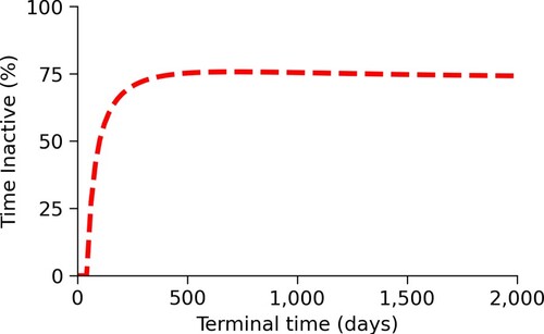
In Figure 7, we see that the proportion of time spent at the minimum mixing level initially increases as the terminal time T increases, but eventually, begins to decrease. For larger T, about 75% of the time is spent at the least active mixing level.

Figure 7. Changes in the proportion of time spent at the minimum mixing level due to changes in the time horizon. This figure shows that the proportion of time spent at the minimum mixing level initially increases quickly as the terminal time, T, increases. At around T=200 days, this increase slows down. At about T=650 days, the proportion of time spent at the minimum mixing level begins to slowly decrease.

5.2. Sensitivity with respect to disease parameters

Next, we would like to see how changes in parameter values relating to the disease under study affect the optimal switching time for the mixing level. If these changes are significant, it may indicate that promoting mitigation strategies other than reduced mixing could be economically beneficial.

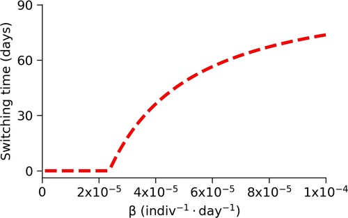
5.2.1. Effects of varying β

The first parameter we will look at is β, the transmission coefficient. In Figure 8, we vary β and find that decreasing the transmission coefficient means that mixing levels can be raised sooner, as expected. Since the value of β estimated from [63] is around $0.463\times {10}^{-4}(\mathrm{i}\mathrm{n}\mathrm{d}\mathrm{i}\mathrm{v}\cdot \mathrm{d}\mathrm{a}\mathrm{y}{)}^{-1}$, using mitigation strategies that further reduce transmission may be effective.

Figure 8. Changes in switching time, $t_1$, due to changes in β. We see that the switching time decreases quickly when we decrease the transmission coefficient, β, from the baseline value.

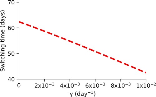
5.2.2. Effects of varying γ

Another parameter that affects the spread of a disease is γ, the per-capita rate of recovery. As we increase γ, infected individuals recover sooner and reenter the susceptible pool faster. Figure 9 shows that, as we increase γ, the optimal switching time decreases. Therefore, decreasing the time to recover by developing effective treatment strategies is a beneficial mitigation strategy.

Figure 9. Changes in switching time, $t_1$, due to changes in γ. We see that as the per-capita recovery rate, γ, increases from $1.0\times {10}^{-6}{\mathrm{d}\mathrm{a}\mathrm{y}}^{-1}$ to $1.0\times {10}^{-2}{\mathrm{d}\mathrm{a}\mathrm{y}}^{-1}$, the optimal switching time decreases from about 62 days to 42 days.

5.2.3. Effects of varying $I_0$

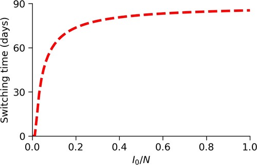
Lastly, it is common for a disease to spread through a significant proportion of a population before mitigation strategies are implemented. Therefore, we determine how varying the initial number of infected individuals changes the optimal switching time. Figure 10 shows that if a greater proportion of the population is infected before reduced mixing strategies are implemented, mixing levels should be reduced for longer.

Figure 10. Changes in switching time, $t_1$, due to changes in $I_0$. We see that as the initial number of infectives, $I_0$, increases from 0.001N individuals to 1.0N individuals, the optimal switching time increases quickly from 0 days (always active) to 85 days.

5.3. Sensitivity of the objective functional

Although the switching time is our key output and thus, the focus of our analysis, we also explore the effects of changes in parameter values on the objective functional. The figures showing these sensitivity analyses are included in the Supplementary Material. In general, the changes in the objective functional with respect to the disease parameters are as expected. Changes in the optimal control parameters can cause payoff to both increase and decrease.

6. Discussion

In this study, we formulated an optimal-control problem for maximizing economic output during an infectious-disease outbreak. We studied a problem that obeys SIS dynamics, and we allowed the level of mixing in the population to range from the lowest possible level of mixing to the highest possible level of mixing.

We determined that the optimal solution used bang-bang controls. This meant that the population was either at its highest level of mixing or its lowest level of mixing at any point in time. We also found that there was at most one switch and that the population had to be at the highest level of mixing at the time horizon. This meant that there was either one switch from low mixing to high mixing or the population remained at the higher level for all times.

We were able to determine analytical solutions for our optimal-control problem, but we were not able to solve for the switching time explicitly. We were, however, able to determine the ratio of the revenue and cost parameters as a function of the switching time. From this, we found that if the ratio of the revenue and cost parameters was small, the population remained at the lower mixing level for longer. As the ratio increased, the switching time occurred sooner. This result emphasizes the importance of correctly identifying the revenue and cost parameters when working with real-world examples.

Next, we studied S. aureus GTB transmission using both numerical methods and our analytical solutions. We saw that the economic output was maximized when mixing was reduced for about half of the simulation. Furthermore, for our example, we found that while mixing was reduced, the outbreak was controlled and that once the switch occurred, the number of cases began to increase. We again emphasize that we studied a mild disease. For a potentially fatal disease, the cost parameter should be chosen to properly account for loss of life.

Finally, we analyzed how changes in parameter values affected the optimal switching time. For our example, we found that the optimal switching time decreased as the ratio of the revenue and cost parameters increased. Also, we found that when the revenue parameter was 0.2 times the cost parameter, no switch would occur. The optimal switching time increased as the values of the minimum and maximum mixing levels increased. This effect was stronger for the minimum mixing level. Also, the switching time increased with the time horizon. For our disease parameters, we saw that as the transmission coefficient increased, the switching time rapidly increased towards the terminal time, and the switching time significantly decreased as the per-capita rate of recovery increased. The results of the sensitivity analysis indicate that it is beneficial to employ further mitigation strategies such as improving treatment options or vaccinations. Another parameter that had a strong effect on the switching time was $I_0$, the initial infected population. Since the prevalence of S. aureus infections in a herd can be high, this is an important value to consider when implementing reduced-mixing control strategies.

An important component of this work is that we were able to determine closed-form analytic solutions for the optimal-control problem of maximizing economic output during an outbreak. These solutions, however, are for a simple disease model that assumes a constant population size, does not consider a discount term in the objective functional, and lacks classes such as exposed, vaccinated, or deceased. When performing a similar analysis on infectious diseases with more complex dynamics, it will be much more difficult to obtain closed-form solutions. Future work may include incorporating these more complex dynamics into our optimal-control problem and working with real-world data.

An assumption of our optimal-control problem that may be limiting is the assumption that infected individuals mix with the general population, but do not produce revenue. If isolation is not an option, mixing with the the general population may still occur. We assumed that individuals do not produce revenue when sick as they may be unable to work or to produce usable goods.

If infected individuals can be asymptomatic or can still be productive when symptoms are mild, we can include a parameter, $0\le \sigma \le 1$, that represents disease severity. If $\sigma =1$, the disease is very severe, and if $\sigma =0$, the disease is completely asymptomatic. We can then write the revenue produced by infected individuals as (23) $\underset{m\le a\left(t\right)\le M}{max}{\int }_0^{T}ra\left(t\right)[N-I(t\left)\right]+a\left(t\right)r(1-\sigma )I\left(t\right)-cI\left(t\right)\mathrm{d}t.$(23) In this paper, we assumed $\sigma =1$.

We have recently begun analyzing optimal-control problems using objective functional (23(23) $\underset{m\le a\left(t\right)\le M}{max}{\int }_0^{T}ra\left(t\right)[N-I(t\left)\right]+a\left(t\right)r(1-\sigma )I\left(t\right)-cI\left(t\right)\mathrm{d}t.$(23) ) with various levels of disease severity. So far, we have found that the optimal control is still bang-bang. In this case, however, we have found instances where multiple, coexisting extremals are able to satisfy Pontryagin's maximum principle. Depending on the values of σ and $I_0$, some of these solutions have two switches. Theoretical studies suggest that optimal-control problems can routinely possess coexisting extremals [42,54]. These have, however, rarely, if ever, been reported in numerical optimal-control studies of diseases.

In this study, we focused on determining how a population should behave during an outbreak in order to maximize economic output. The population size we used is on a business or farm level. This problem can be scaled up to represent larger populations, such as a region or country, or scaled down to represent even smaller communities. The scale of the problem can be changed by changing parameters like the population size, the revenue parameter, and the cost parameter. A population of any size, however, is not homogeneous in risk of infection and in the consequences of infection. For example, an individual who is able to work from home may behave differently during an epidemic than an individual who must work in-person. Moreover, a large dairy farm in good financial standing may be able to use different reduced-mixing strategies than a smaller dairy farm. Therefore, an interesting follow-up question to this research is what an individual's optimal strategy might be during an infectious-disease outbreak.

Funding 

The author(s) reported there is no funding associated with the work featured in this article.

Acknowledgments

We would like to thank the anonymous reviewers and the editor for their helpful comments.

Disclosure statement

No potential conflict of interest was reported by the author(s).

References

- N.T.J. Bailey, The Mathematical Theory of Epidemics, Charles Griffin and Co. Ltd., London, 1957.
- R.E. Baker, A.S. Mahmud, I.F.M.M. Rajeev, F. Rasambainarivo, B.L. Rice, S. Takahashi, A.J. Tatem, C.E. Wagner, L.F. Wang, A. Wesolowski, and C.J.E. Metcalf, Infectious disease in an era of global change, Nat. Rev. Microbiol. 20 (2021), pp. 193–205.
- N.G. Becker, Modeling to Inform Infectious Disease Control, Chapman and Hall/CRC, Boca Raton, 2015.
- J. Bedford, J. Farrar, C. Ihekweazu, G. Kang, M. Koopmans, and J. Nkengasong, A new twenty-first century science for effective epidemic response, Nature 575 (2019), pp. 130–136.
- P. Beutels, N. Jia, Q.Y. Zhou, R. Smith, W.C. Cao, and S.J. de Vlas, The economic impact of SARS in Beijing, China, Trop. Med. Int. Health. 14 (2009), pp. 85–91.
- P.A. Bliman and M. Duprez, How best can finite-time social distancing reduce epidemic final size? J. Theoret. Biol. 511 (2021), p. 110557.
- L. Bolzoni, E. Bonacini, C. Soresina, and M. Groppi, Time-optimal control strategies in SIR epidemic models, Math. Biosci. 292 (2017), pp. 86–96.
- M.L. Brandeau, Allocating resources to control infectious diseases, in Operations Research and Health Care, International Series in Operations Research and Management Science, Vol. 70, M.L. Brandeau, F. Sainfort, and W.P. Pierskalla, eds., Chap. 17, Springer, Boston, MA, 2005, pp. 443–464.
- F. Brauer, C. Castillo-Chavez, and Z. Feng, Mathematical Models in Epidemiology, Springer, New York, 2019.
- N.F. Britton, Essential Mathematical Biology, Springer, London, 2003.
- E.H. Bussell, C.E. Dangerfield, C.A. Gilligan, and N.J. Cunniffe, Applying optimal control theory to complex epidemiological models to inform real-world disease management, Philos. Trans. Roy. Soc. B 374 (2019), p. 20180284.
- C. Castillo-Chavez, W. Huang, and J. Li, Competitive exclusion in gonorrhea models and other sexually transmitted diseases, SIAM J. Appl. Math. 56 (1996), pp. 494–508.
- W.N. Cheng and S.G. Han, Bovine mastitis: risk factors, therapeutic strategies, and alternative treatments – a review, Asian-Australas. J. Anim. Sci. 33 (2020), pp. 1699–1713.
- P.G. Coen, A.G. Luckins, H.C. Davison, and M.E.J. Woolhouse, Trypanosoma evansi in Indonesian buffaloes: evaluation of simple models of natural immunity to infection, Epidemiol. Infect. 126 (2001), pp. 111–118.
- P. Corredor-Moreno and D.G.O. Saunders, Expecting the unexpected: factors influencing the emergence of fungal and oomycete plant pathogens, New Phytol. 225 (2020), pp. 118–125.
- N.J. Cunniffe, F.F. Laranjeira, F.M. Neri, R.E. DeSimone, and C.A. Gilligan, Cost-effective control of plant disease when epidemiological knowledge is incomplete: modelling Bahia bark scaling of citrus, PLOS Comput. Biol. 10 (2014), p. e1003753.
- V.G. da Costa, M.L. Moreli, and M.V. Saivish, The emergence of SARS, MERS and novel SARS-2 coronaviruses in the 21st century, Arch. Virol. 165 (2020), pp. 1517–1526.
- D.J. Daley and J. Gani, Epidemic Modelling: An Introduction, Cambridge University Press, Cambridge, 1999.
- L.K. Dixon, H. Sun, and H. Roberts, African swine fever, Antiviral Res. 165 (2019), pp. 34–41.
- B.C. Fabien, Dsoa: the implementation of a dynamic system optimization algorithm, Optimal Control Appl. Methods 31 (2010), pp. 231–247.
- E.P. Fenichel, C. Castillo-Chavez, M.G. Ceddia, G. Chowell, P.A.G. Parra, G.J. Hickling, G. Holloway, R. Horan, B. Morin, C. Perrings, M. Springborn, L. Velazquez, and C. Villalobos, Adaptive human behavior in epidemiological models, Proc. Natl. Acad. Sci. USA 108 (2011), pp. 6306–6311.
- H. Gaff and E. Schaefer, Optimal control applied to vaccination and treatment strategies for various epidemiological models, Math. Biosci. Eng. 6 (2009), pp. 469–492.
- M. Gambhir, M.G. Basáñez, M.J. Burton, A.W. Solomon, R.L. Bailey, M.J. Holland, I.M.Blake, C.A. Donnelly, I. Jabr, D.C. Mabey, and N.C. Grassly, The development of an age-structured model for trachoma transmission dynamics, pathogenesis and control, PLoS Negl. Trop. Dis. 3 (2009), p. e462.
- J. González-Guzmán, An epidemiological model for direct and indirect transmission of typhoid fever, Math. Biosci. 96 (1989), pp. 33–46.
- T. Halasa, K. Huijps, O. Østerås, and H. Hogeveen, Economic effects of bovine mastitis and mastitis management: a review, Vet. Q. 29 (2007), pp. 18–31.
- S.E. Heath, The impact of epizootics on livelihoods, J. Appl. Anim. Welf. Sci. 11 (2008), pp. 98–111.
- H.W. Hethcote, Three basic epidemiological models, in Applied Mathematical Ecology, S.A. Levin, T.G. Hallam, and L.J. Gross, eds., Springer, Berlin, Heidelberg, 1989, pp. 119–144.
- H. Hethcote and J. Yorke, Gonorrhea transmission dynamics and control, Lect. Notes Biomath. 56 (1984), pp. 18–24.
- C.R.R. Hooks and A. Fereres, Protecting crops from non-persistently aphid-transmitted viruses: a review on the use of barrier plants as a management tool, Virus Res. 120 (2006), pp. 1–16.
- A.D. James and J. Rushton, The economics of foot and mouth disease, Rev. Sci. Tech. 21 (2002), pp. 637–644.
- K.E. Jones, N.G. Patel, M.A. Levy, A. Storeygard, D. Balk, J.L. Gittleman, and P. Daszak, Global trends in emerging infectious diseases, Nature 451 (2008), pp. 990–993.
- R.A.C. Jones, Using epidemiological information to develop effective integrated virus disease management strategies, Virus Res. 100 (2004), pp. 5–30.
- S. Kalra, D. Kelkar, S.C. Galwankar, T.J. Papadimos, S.P. Stawicki, B. Arquilla, B.A. Hoey, R.P.Sharpe, D. Sabol, and J.A. Jahre, The emergence of ebola as a global health security threat: from ‘lessons learned’ to coordinated multilateral containment efforts, J. Glob. Infect. Dis. 6 (2014), pp. 164–177.
- M.J. Keeling and P. Rohani, Modeling Infectious Diseases in Humans and Animals, Princeton University Press, Princeton, 2008.
- W.O. Kermack and A.G. McKendrick, A contribution to the mathematical theory of epidemics, Proc. R. Soc. Lond. A 115 (1927), pp. 700–721.
- C. Klap, N. Luria, E. Smith, E. Bakelman, E. Belausov, O. Laskar, O. Lachman, A. Gal-On, and A.Dombrovsky, The potential risk of plant-virus disease initiation by infected tomatoes, Plants 9 (2020), p. 623.
- T.J.D. Knight-Jones and J. Rushton, The economic impacts of foot and mouth disease – what are they, how big are they and where do they occur? Prev. Vet. Med. 112 (2013), pp. 161–173.
- S. Lenhart and J.T. Workman, Optimal Control Applied to Biological Models, Chapman and Hall/CRC, Boca Raton, 2007.
- F. Lin, K. Muthuraman, and M. Lawley, An optimal control theory approach to non-pharmaceutical interventions, BMC Infect. Dis. 10 (2010), pp. 32.
- R. Mazzucco, U. Dieckmann, and J.A.J. Metz, Epidemiological, evolutionary, and economic determinants of eradication tails, J. Theoret. Biol. 405 (2016), pp. 58–65.
- G. Neumann, T. Noda, and Y. Kawaoka, Emergence and pandemic potential of swine-origin H1N1 influenza virus, Nature 459 (2009), pp. 931–939.
- C. Offen and S. Ober-Blöbaum, Bifurcation preserving discretisations of optimal control problems, IFAC-PapersOnLine 54 (2021), pp. 334–339.
- T.C. Pierson and M.S. Diamond, The emergence of Zika virus and its new clinical syndromes, Nature 560 (2018), pp. 573–581.
- L.S. Pontryagin, V.G. Boltyanskii, R.V. Gamkrelidze, and E.F. Mishchenko, The Mathematical Theory of Optimal Processes, John Wiley & Sons, New York, 1962.
- J.D. Porter and K.P. McAdam, The re-emergence of tuberculosis, Annu. Rev. Public Health 15 (1994), pp. 303–323.
- W.J.M. Probert, K. Shea, C.J. Fonnesbeck, M.C. Runge, T.E. Carpenter, S. Dürr, M.G. Garner, N.Harvey, M.A. Stevenson, C.T. Webb, M. Werkman, M.J. Tildesley, and M.J. Ferrari, Decision-making for foot-and-mouth disease control: objectives matter, Epidemics 15 (2016), pp. 10–19.
- S. Pyörälä, Treatment of mastitis during lactation, Ir. Vet. J. 62 (2009), p. 40.
- J.B. Ristaino, P.K. Anderson, D.P. Bebber, K.A. Brauman, N.J. Cunniffe, N.V. Fedoroff, C. Finegold, K.A. Garrett, C.A. Gilligan, C.M. Jones, M.D. Martin, G.K. MacDonald, P. Neenan, A. Records, D.G.Schmale, L. Tateosian, and Q. Wei, The persistent threat of emerging plant disease pandemics to global food security, Proc. Natl. Acad. Sci. USA 118 (2021), p. e2022239118.
- E. Rollin, K.C. Dhuyvetter, and M.W. Overton, The cost of clinical mastitis in the first 30 days of lactation: an economic modeling tool, Prev. Vet. Med. 122 (2015), pp. 257–264.
- J. Rushton, P.K. Thornton, and M.J. Otte, Methods of economic impact assessment, Rev. Sci. Tech.18 (1999), pp. 315–342.
- S. Saha, G.P. Samanta, and J.J. Nieto, Epidemic model of COVID-19 outbreak by inducing behavioural response in population, Nonlinear Dyn. 102 (2020), pp. 455–487.
- S. Saha, G.P. Samanta, and J.J. Nieto, Impact of optimal vaccination and social distancing on COVID-19 pandemic, Math. Comput. Simul. 200 (2022), pp. 285–314.
- K. Schneider, W. van der Werf, M. Cendoya, M. Mourits, J.A. Navas-Cortés, A. Vicent, and A.O.Lansink, Impact of Xylella fastidiosa subspecies pauca in European olives, Proc. Natl. Acad. Sci. USA117 (2020), pp. 9250–9259.
- S.Y. Serovaiskii, Counterexamples in Optimal Control Theory, De Gruyter, Berlin, Boston, 2011.
- S.P. Sethi, Optimal quarantine programmes for controlling an epidemic spread, J. Oper. Res. Soc. 29 (1978), pp. 265–268.
- S. Sharma, A. Mondal, A.K. Pal, and G.P. Samanta, Stability analysis and optimal control of avian influenza virus a with time delays, Int. J. Dyn. Control 6 (2018), pp. 1351–1366.
- S. Sharma and G.P. Samanta, Analysis of a chlamydia epidemic model, J. Biol. Syst. 22 (2014), pp. 713–744.
- O. Sharomi and T. Malik, Optimal control in epidemiology, Ann. Oper. Res. 251 (2017), pp. 55–71.
- E. Shim, Optimal strategies of social distancing and vaccination against seasonal influenza, Math. Biosci. Eng. 10 (2013), pp. 1615–1634.
- K.F. Smith, M. Goldberg, S. Rosenthal, L. Carlson, J. Chen, C. Chen, and S. Ramachandran, Global rise in human infectious disease outbreaks, J. R. Soc. Interface 11 (2014), p. 20140950.
- P.J. Sánchez-Cordón, M. Montoya, A.L. Reis, and L.K. Dixon, African swine fever: a re-emerging viral disease threatening the global pig industry, Vet. J. 233 (2018), pp. 41–48.
- F.M. Tomley and M.W. Shirley, Livestock infectious diseases and zoonoses, Philos. Trans. R. Soc. Lond., B, Biol. Sci. 364 (2009), pp. 2637–2642.
- B.H. van den Borne, H.U. Graber, V. Voelk, C. Sartori, A. Steiner, M.C. Haerdi-Landerer, and M.Bodmer, A longitudinal study on transmission of staphylococcus aureus genotype B in Swiss communal dairy herds, Prev. Vet. Med. 136 (2017), pp. 65–68.
- R.A. Weiss and A.J. McMichael, Social and environmental risk factors in the emergence of infectious diseases, Nat. Med. 10 (2004), pp. S70–6.
- K. Wickwire, Mathematical models for the control of pests and infectious diseases: a survey, Theor. Popul. Biol. 11 (1977), pp. 182–238.
- D.J. Wilson, R.N. Gonzalez, and P.M. Sears, Segregation or use of separate milking units for cows infected with staphylococcus aureus: effects on prevalence of infection and bulk tank somatic cell count, J. Dairy Sci. 78 (1995), pp. 2083–2085.
- S. Zhang, J.S. Griffiths, G. Marchand, M.A. Bernards, and A. Wang, Tomato brown rugose fruit virus: an emerging and rapidly spreading plant RNA virus that threatens tomato production worldwide, Mol. Plant Pathol. 23 (2022), pp. 1262–1277.