A contact tracing SIR model for randomly mixed populations

Abstract

Contact tracing is an important intervention measure to control infectious diseases. We present a new approach that borrows the edge dynamics idea from network models to track contacts included in a compartmental SIR model for an epidemic spreading in a randomly mixed population. Unlike network models, our approach does not require statistical information of the contact network, data that are usually not readily available. The model resulting from this new approach allows us to study the effect of contact tracing and isolation of diagnosed patients on the control reproduction number and number of infected individuals. We estimate the effects of tracing coverage and capacity on the effectiveness of contact tracing. Our approach can be extended to more realistic models that incorporate latent and asymptomatic compartments.

Keywords:

• Compartmental disease model
• control reproduction number
• pair dynamics
• tracing coverage
• tracing capacity

1. Introduction

The introduction of a novel or rare transmissible pathogen into a susceptible population requires strong measures to control or prevent ongoing transmission. Recent examples include Ebola virus, the novel coronavirus causing severe acute respiratory syndrome (SARS), and the novel coronavirus SARS-CoV-2 causing coronavirus disease (COVID-19). Depending on the pathogen, these measures include pharmaceutical interventions (e.g. vaccination and antivirals) or non-pharmaceutical interventions (e.g. social distancing, mask-wearing, ventilation, business and school closures, and contact tracing). Specifically, contact tracing is a crucial public health intervention strategy for emerging and re-emerging infectious diseases to contain and prevent the further spread of the disease [16, 27]. Following the testing and isolation of a positively diagnosed infectious case, contact tracing is initiated: contacts of the diagnosed case are identified for quarantine and subsequent testing and isolation are undertaken as required. The isolation of infectious individuals during their infectious period is crucial for inhibiting further transmission. Studies have shown that contact tracing can be effective in reducing the control reproduction number ${\mathcal{R}}_c$ of SARS-CoV-2, delaying the epidemic peak, and decreasing the epidemic growth rate, particularly in the presence of other non-pharmaceutical interventions; however, contact tracing on its own may not be able to adequately control an epidemic [6, 10–12, 15, 22].

There are challenges and limitations that can impact the effectiveness of contact tracing measures. In the initial stages of an emerging outbreak, proper laboratory diagnostics may not be readily available and must be developed before being able to correctly diagnose infected patients [4, 34]. As well, case definitions, testing criteria, isolation procedures, and other public health interventions may vary over time in terms of their implementation [28, 34].

Contact tracing effectiveness is dependent on the proportion of transmission occurring from individuals in a pre-symptomatic or asymptomatic stage of disease as well as the number of secondary infections resulting from one infectious individual [6, 10]. For example, if a pathogen such as SARS-CoV-2 can be transmitted during a pre-symptomatic stage or from a fully asymptomatic infected individual [32] but guidelines for testing and isolation of infectious cases are based on symptomatic criteria alone, subsequent contact tracing activities may not capture a large fraction of infectious individuals that are contributing to the growing number of community-based infections in the population; thus, the epidemic may not be contained in this scenario [12]. Additionally, the evolution of pathogen characteristics over time can lead to changes in transmission capabilities and disease presentation. For example, the transmissibility and infectiousness of SARS-CoV-2 variants over the course of the COVID-19 pandemic have varied greatly [5, 23]. As infections increase, there may also be challenges in maintaining appropriate and sustainable resources and capacity levels. Laboratories may be hindered in their ability to undertake timely and accurate testing and contact tracers may become overwhelmed in attempting to identify contacts in a timely fashion [3].

Mathematical models can be used to examine the impact of contact tracing and testing on disease dynamics in terms of the magnitude and duration of transmission of an infectious pathogen in a population [8, 22, 24]. One approach is the use of compartmental models. Those that assume a random mixing population, such as the Kermack–McKendrick susceptible-infected-removed (SIR) model and their extensions, have been widely used to study disease dynamics [2, 19, 26, 33]. However, while some of these models incorporate contact tracing they are not precise because they do not track the contacts of patients, which is crucial in understanding contact tracing [18, 31, 33]. In fact, these models assume that a constant fraction of new infections will be traced; however, realistically this fraction increases with the number of traced patients. Other powerful approaches that mathematically model contact tracing are stochastic models, e.g. [15, 17, 21]. These models have been used to study the effect of contact tracing on the reduction of secondary infections (the reproduction number). However, it can be difficult to use stochastic models to study the dynamics of epidemics. Similarly, contact networks are used to study contact tracing because they keep track of neighbours [7, 11, 13, 20]. However, applying contact networks to disease dynamics requires a detailed understanding of the underlying network structure, such as the degree distribution (the distribution of the number of neighbours of a random node) [1, 9], clustering (the fraction of edges in a triangle) [7, 13, 20], degree correlation (whether nodes with many neighbours are likely to connect to each other) [13, 14], and other information on network topology [25, 29]. This network information is not usually easily available. Additionally, while agent-based models can be useful, they require the utilization of many parameters and computational capacity [26].

Instead, we borrow the idea of tracing the states of nodes and their contacts from contact network models to develop a new compartmental model for contact tracing. In this model, we keep track of the states of the patient and the infector together in a pair. This novel approach allows us to determine the rate that patients are contact traced. Our new model is introduced in Section 2. For validation, in Section 3, we introduce an agent-based model for contact tracing of an SIR epidemic, which is used to compare the simulations with the solutions of our model. In Section 4, the control reproduction number is calculated, and the model dependence on the contact tracing parameters is discussed. The effect of tracing capacity is considered in Section 5, with concluding remarks given in Section 6.

2. The compartmental SIR contact tracing model

We consider susceptible-infected-recovered (SIR) epidemic spread in a randomly mixed population that is subject to testing and contact tracing. The population is divided into the susceptible (S), infectious (I), diagnosed (T for tested positive), contact tracing initiated (X), and recovered and not diagnosed (R) classes. We assume that voluntary testing is initiated by infectious symptomatic individuals and thus we ignore asymptomatic and pre-symptomatic disease states. In addition, we assume that the diagnosed patients (T) and contact traced individuals (X) are fully isolated, and do not transmit disease. We assume that disease deaths are negligible, and are thus not considered here. We also ignore the population dynamics, so that the population size N remains constant. Assuming a randomly mixed population, T is typically a small fraction of the total population, and the number of contact traced (and quarantined) susceptible individuals is also a small fraction of the population. Therefore, these quarantined susceptible individuals have a negligible effect on disease dynamics. Thus, we ignore the contact tracing and quarantining of susceptible individuals. We also assume that contact tracing has no effect on a T, X or R contact.

2.1. Tree of transmission

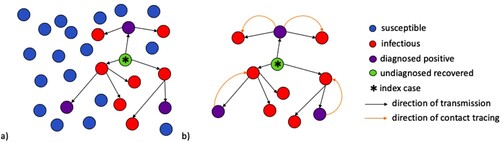
We consider disease transmission in a randomly mixed population; specifically, the tree of transmission in such a population. Figure 1 provides a visualization of the chain of infections occurring from the introduction of an infectious individual (or node) in a population of susceptible individuals (or nodes). The direction of the arrows in Figure 1(a) shows the direction of transmission, or, who-infected-who. The purple nodes reflect those who have been infected and positively diagnosed. We can ignore the remaining susceptible nodes and examine the remaining tree of transmission and apply contact tracing (Figure 1(b)). Notice that each individual node that has been infected is part of a pair of nodes. Here, the orange arrows reflect the direction of contact tracing that has been initiated from the positively diagnosed node. We now want to study this tree of transmission when diagnosis and contact tracing occur.

Figure 1. (a) A population of randomly mixed nodes. The arrows between the nodes denote the chain of transmission within the population following the introduction of an initial infectious node (*). Purple nodes represent infectious nodes that have been tested and diagnosed positive. The red nodes are infectious but undiagnosed. The green node represents recovery of an infectious node that has not been diagnosed. (b) A tree of transmission resulting from interactions between infectious and susceptible nodes. The orange arcs represent the direction of contact tracing triggered from a positively diagnosed node.

2.2. Model development

To model contact tracing, we keep track of contacts that caused infections. These contacts form a tree of infections, where the nodes are the patients, and arcs represent who-infected-who. The infection process generates this tree dynamically, while the contact tracing operates on the tree. An edge on the tree is labelled as $[A\leftarrow B]$, representing a node of class A that was infected by a node currently in class B where $A,B\in \{I,T,X,R\}$, e.g. $[I\leftarrow I]$, $[I\leftarrow T]$, $[T\leftarrow I]$, etc. Here, the direction of the arrow denotes the direction of transmission. A diagnosed patient (T) initiates contact tracing (and becomes X) at a rate θ, and their I contacts are traced with probability p and become diagnosed (T). Thus, the $[I\leftarrow T]$ and $[T\leftarrow I]$ pairs become $[T\leftarrow X]$ and $[X\leftarrow T]$, respectively, at a rate $\theta p$. This process then propagates to all I neighbours of the newly diagnosed node.

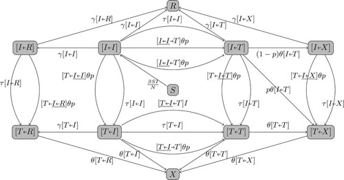
Figure 2 shows the flowchart of the population dynamics. As in a standard SIR model, the susceptible individuals (S) are infected and become infectious patients according to $S^{\prime }=-\text{β}\frac{SI}{N},$where β is the transmission rate, and N is the total population size. A patient (I) may:

• recover and become R at a rate γ; or,

• be diagnosed positive and become T at a rate τ; or,

• be traced and also become T either in:

  • an $[I\leftarrow T]$ pair if their infector is diagnosed (T); or,

  • in a $[T\leftarrow I]$ pair if one of the contacts they infected is T.

Figure 2. Flowchart of SIR model with testing and tracing (Population Dynamics).

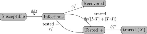
We assume that a T individual triggers contact tracing at a rate θ and becomes X. We also assume that a fraction p of the contacts (independent of their state) of a T individual is captured by contact tracing. This fraction p is called the coverage probability. Then, $\begin{array}{rl}{I}^{\prime }& =\text{β}\frac{SI}{N}-\gamma I-\tau I-\theta p\left(\right[I\leftarrow T]+[T\leftarrow I\left]\right),\\ T^{\prime }& =\tau I+\theta p\left(\right[I\leftarrow T]+[T\leftarrow I\left]\right)-\theta T,\\ X^{\prime }& =\theta T,\\ R^{\prime }& =\gamma I.\end{array}$

To model the dynamics of the pairs $[I\leftarrow T]$ and $[T\leftarrow I]$ (Figure 3), we start with the dynamics of an $[I\leftarrow I]$ pair that is formed when a susceptible individual is infected. Both $[I\leftarrow T]$ and $[T\leftarrow I]$ pairs come from an $[I\leftarrow I]$ pair. In an $[I\leftarrow I]$ pair, the first I is the new patient and the second is the infector. There are several possibilities for how the state of an $[I\leftarrow I]$ pair changes:

• the patient recovers at a rate γ and enters R; or,

• the infector recovers at a rate γ and the pair becomes $[I\leftarrow R]$; or,

• the patient is voluntarily tested and diagnosed at a rate τ and the pair becomes $[T\leftarrow I]$ (while the patient enters T); or,

• the infector is tested at a rate τ and the pair becomes $[I\leftarrow T]$; or,

• the patient or the infector is contact-traced (described below).

Figure 3. Flowchart of Pair Dynamics.

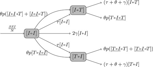
The infectee in an $[I\leftarrow I]$ pair may be contact traced from one of their secondary infections, which happens in a triple interaction $[T\leftarrow \underset{\_}{I\leftarrow I}]$ (the underline represents the original $[I\leftarrow I]$ pair). Similarly, the infector may be traced from their infector in triples $[\underset{\_}{I\leftarrow I}\leftarrow T]$, or from another of their secondary infections in $[\underset{\_}{I\leftarrow I}\to T]$. Each of these triple interactions occurs at a rate $\theta p$ (because the patient is captured by contact tracing with a probability p).

Thus, $[I\leftarrow I{]}^{\prime }=\text{β}\frac{SI}{N}-(2\gamma +2\tau \left)\right[I\leftarrow I]-\theta p([T\leftarrow \underset{\_}{I\leftarrow I}]+[\underset{\_}{I\leftarrow I}\leftarrow T]+[\underset{\_}{I\leftarrow I}\to T]).$We also track the dynamics of the triple interactions $[T\leftarrow \underset{\_}{I\leftarrow I}]$, $[\underset{\_}{I\leftarrow I}\leftarrow T]$ and $[\underset{\_}{I\leftarrow I}\to T]$. Their dynamics further depend on the interactions of four individuals. Eventually, the full interaction dynamics give an infinite-dimensional system. Instead, we use a closure method that has commonly been used in network models [30]. For example, a $[T\leftarrow \underset{\_}{I\leftarrow I}]$ triple is a $[T\leftarrow I]$ pair followed by an $[I\leftarrow I]$ pair. Thus, the number of $[T\leftarrow \underset{\_}{I\leftarrow I}]$ triples is the product of the number of $[T\leftarrow I]$ pairs and the average number of $[I\leftarrow I]$ pairs where the infector of the $[T\leftarrow I]$ pair is a patient. From the random mixing assumption, the average number of $[I\leftarrow I]$ pairs following an I can be approximated as $[I\leftarrow I]/I$. Thus, $[T\leftarrow \underset{\_}{I\leftarrow I}]\approx [T\leftarrow I]\frac{[I\leftarrow I]}{I}.$Similarly, $[\underset{\_}{I\leftarrow I}\leftarrow T]\approx [I\leftarrow I]\frac{[I\leftarrow T]}{I}.$The number of $[\underset{\_}{I\leftarrow I}\to T]$ triples is the product of the number of $[I\leftarrow I]$ pairs and the average number of $[T\leftarrow I]$ pairs when the infector of the $[I\leftarrow I]$ pair has infected the T in the $[T\leftarrow I]$ pair. That is, $[\underset{\_}{I\leftarrow I}\to T]\approx [I\leftarrow I]\frac{[T\leftarrow I]}{I}.$For the dynamics of the $[I\leftarrow T]$ pair, they come from $[I\leftarrow I]$ pairs as stated above. The patient may recover and become R at a rate γ, or may become $[T\leftarrow T]$ if the patient is either tested and diagnosed with a rate τ or contact traced. In the last case, the contact tracing may be initiated by the infector (and then the pair becomes either $[T\leftarrow X]$ with a probability p if the patient is successfully traced, or $[I\leftarrow X]$ otherwise), or initiated by another T infected by the patient in a $[T\leftarrow \underset{\_}{I\leftarrow T}]$ triple interaction. And thus, $\begin{array}{rl}[I\leftarrow T{]}^{\prime }& =\tau [I\leftarrow I]+\theta p\left(\right[\underset{\_}{I\leftarrow I}\to T]+[\underset{\_}{I\leftarrow I}\leftarrow T\left]\right)-(\gamma +\tau +\theta )[I\leftarrow I]\\ & -\theta p[T\leftarrow \underset{\_}{I\leftarrow T}],\end{array}$where $[T\leftarrow \underset{\_}{I\leftarrow T}]=[T\leftarrow I]\frac{[I\leftarrow T]}{I}.$Finally, a $[T\leftarrow I]$ pair also comes from an $[I\leftarrow I]$ pair, and may become $[T\leftarrow R]$ if the infector recovers, or $[T\leftarrow T]$ if the infector either tests positive or is traced (from either the T patient in the pair, or a T infector in a $[\underset{\_}{T\leftarrow I}\leftarrow T]$ triple, or another T contact in a $[\underset{\_}{T\leftarrow I}\to T]$ triple. Thus, $\begin{array}{rl}[T\leftarrow I{]}^{\prime }& =\tau [I\leftarrow I]+\theta p[T\leftarrow \underset{\_}{I\leftarrow I}]-(\gamma +\tau +\theta )[T\leftarrow I]-\theta p\left(\right[\underset{\_}{T\leftarrow I}\leftarrow T]\\ & +[\underset{\_}{T\leftarrow I}\to T]),\end{array}$where $[\underset{\_}{T\leftarrow I}\leftarrow T]=[T\leftarrow I]\frac{[I\leftarrow T]}{I}=[T\leftarrow \underset{\_}{I\leftarrow T}],[\underset{\_}{T\leftarrow I}\to T]=[T\leftarrow I]\frac{[T\leftarrow I]}{I}.$Therefore, the system can be written as below: (1a) $\begin{array}{rl}{S}^{\prime }& =-\text{β}S\frac{I}{N},\end{array}$(1a) (1b) $\begin{array}{rl}{I}^{\prime }& =\text{β}S\frac{I}{N}-(\gamma +\tau )I-\theta p\left(\right[I\leftarrow T]+[T\leftarrow I\left]\right),\end{array}$(1b) (1c) $\begin{array}{rl}[I\leftarrow I{]}^{\prime }& =\text{β}S\frac{I}{N}-2(\gamma +\tau )[I\leftarrow I]-\theta p\frac{2[T\leftarrow I]+[I\leftarrow T]}{I}[I\leftarrow I],\end{array}$(1c) (1d) $\begin{array}{rl}[I\leftarrow T{]}^{\prime }& =\tau [I\leftarrow I]+\theta p\frac{[I\leftarrow T]+[T\leftarrow I]}{I}[I\leftarrow I]-(\gamma +\tau +\theta )[I\leftarrow T]\\ & -\theta p\frac{[T\leftarrow I][I\leftarrow T]}{I},\end{array}$(1d) (1e) $\begin{array}{rl}[T\leftarrow I{]}^{\prime }& =\tau [I\leftarrow I]+\theta p\frac{[T\leftarrow I][I\leftarrow I]}{I}-(\gamma +\tau +\theta )[T\leftarrow I]\\ & -\theta p\frac{[T\leftarrow I]+[I\leftarrow T]}{I}[T\leftarrow I],\end{array}$(1e) (1f) $\begin{array}{rl}{T}^{\prime }& =\tau I+\theta p\left(\right[I\leftarrow T]+[T\leftarrow I\left]\right)-\theta T,\end{array}$(1f) (1g) $\begin{array}{rl}{X}^{\prime }& =\theta T,\end{array}$(1g) (1h) $\begin{array}{rl}{R}^{\prime }& =\gamma I.\end{array}$(1h) Figure A1 in Appendix 1 gives the flowchart of the model tracking all pairs for which the patient is an I or T. The I and T populations are $I=[I\leftarrow I]+[I\leftarrow T]+[I\leftarrow X]+[I\leftarrow R]$ and $T=[T\leftarrow I]+[T\leftarrow T]+[T\leftarrow X]+[T\leftarrow R]$.

3. Model verification

To verify that the model is a good description of the contact tracing process, we constructed an agent-based simulation model for a contact tracing process in a randomly mixed population and showed that the ensemble average of the agent-based simulation agrees with the solutions of model (1a(1a) $\begin{array}{rl}{S}^{\prime }& =-\text{β}S\frac{I}{N},\end{array}$(1a) ).

Consider a population with N individuals. Initially, $I_0$ individuals are randomly selected and labelled infectious (I), while others are labelled susceptible (S). Each infectious individual maintains a list of contacts (that is initially empty). Upon becoming infectious, the individual is assigned four events. The event times are calculated as the current time (of becoming infectious) plus a waiting time. The events are

• a transmission event with a waiting time randomly drawn from an exponential distribution with a rate β;

• a recovery event with a waiting time (i.e. the infectious period) randomly drawn from a probability distribution with a density $f_I\left(t\right)$;

• a test event with a waiting time randomly drawn from a probability distribution with a density $f_T\left(t\right)$.

• a contact tracing event with waiting time randomly drawn from a probability distribution with a density $f_X\left(t\right)$.

Note that only infectious individuals have events attached. The earliest event of all individuals is determined and the corresponding infectious individual is noted. The current time is then set to the next event time. The states are adjusted according to the following algorithm:

• If it is a transmission event, then a contact is randomly chosen assuming individuals are uniformly distributed in the population. If the contact is susceptible, then the contact becomes infectious. To implement contact tracing, the contact is added to the list of contacts of the infectious individual. The infectious individual is also added to the contact list of the contact. A new contact event with an i.i.d. waiting time is assigned to the infectious individual.

• If it is a recovery event (at the end of the infectious period), the individual is labelled recovered, and the contact list and all remaining events attached to this individual are cleared. A recovered individual obtains lifetime immunity and will not be infected again.

• If it is a test event, then the infectious individual is relabeled diagnosed (T). A contact tracing event with a waiting time drawn from the distribution $f_X\left(t\right)$ is assigned to the diagnosed individual.

• If it is a contact tracing event, each contact in their contact list is traced. If the contact is infectious, then the contact becomes diagnosed with a probability p (i.e. the contact tracing coverage probability). Otherwise, the contact remains intact. The contact tracing process is recursively applied to the contacts. After all the contacts are traced, the contact list and all remaining events attached to this individual are cleared. Thus, we do not keep track of recovery of diagnosed individuals in this process, and diagnosed individuals are fully isolated and do not further infect others.

The earliest event has now been handled. We then inspect the next event. This process is repeated until no event remains, or a designated time is reached in the simulation.

To compare with our compartmental SIR contact tracing model, the infectious period density $f_I\left(t\right)$ is assumed exponential with rate γ, the test waiting time density $f_T\left(t\right)$ is assumed exponential with rate τ, and the contact tracing waiting time density $f_X\left(t\right)$ is assumed exponential with rate θ.

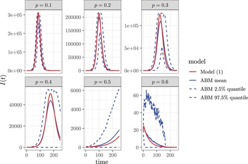
Figure 4 shows the comparison of $I\left(t\right)$ numerically solved from the compartmental SIR contact tracing model (Equation (1a(1a) $\begin{array}{rl}{S}^{\prime }& =-\text{β}S\frac{I}{N},\end{array}$(1a) )-(1h)) with the ensemble average of 100 runs of agent-based simulations with identical parameter values and initial conditions. The numerical solutions of our model agree well with the agent-based simulations, especially in the initial exponential growth phase. Although our model is motivated by the COVID-19 pandemic, it is an oversimplification, and the parameter values are chosen only as a reasonable illustration of results. Time is a continuous variable. The number of infectious individuals is counted at the end of each time step in the simulation.

Figure 4. The comparison of $I\left(t\right)$ numerically solved from our contact tracing model (1a(1a) $\begin{array}{rl}{S}^{\prime }& =-\text{β}S\frac{I}{N},\end{array}$(1a) )-(1h) with the ensemble average of 100 runs of agent-based simulations with identical parameter values and initial conditions. The parameter values are $N=5\times {10}^6$, $\text{β}=0.4$, $\gamma =0.1$, $\tau =0.15$, $\theta =10$, $I\left(0\right)=20$, and the coverage tracing probability (or probability of diagnosis) is $p=0.1,0.2,\dots 0.6$.

4. Model analysis

In this section, we calculate the control reproduction number ${\mathcal{R}}_c$ for the compartmental SIR contact tracing model, and analyse how it depends on the contact tracing parameters.

4.1. Disease-free state and control reproduction number

Without disease (i.e. I = 0), the fractions $[T\leftarrow I]/I$ and $[I\leftarrow T]/I$ are not defined. We change the variables to avoid this problem. Let $u=\frac{[I\leftarrow I]}{I},v=\frac{[I\leftarrow T]}{I},w=\frac{[T\leftarrow I]}{I},$then this system can be rewritten as (2a) $\begin{array}{rl}{S}^{\prime }& =\text{β}S\frac{I}{N}\end{array}$(2a) (2b) $\begin{array}{rl}{I}^{\prime }& =\text{β}S\frac{I}{N}-(\gamma +\tau )I-\theta p(v+w)I,\end{array}$(2b) (2c) $\begin{array}{rl}{u}^{\prime }& =\text{β}\frac{S}{N}(1-u)-(\tau +\gamma )u-\theta puw,\end{array}$(2c) (2d) $\begin{array}{rl}{v}^{\prime }& =\tau u+\theta pu(v+w)-(\text{β}+\theta )v+\theta p{v}^2,\end{array}$(2d) (2e) $\begin{array}{rl}{w}^{\prime }& =\tau u-(\text{β}+\theta )w+\theta puw.\end{array}$(2e) For this system, the set $\{S=N,I=0\}$ is invariant. In addition, $\mathcal{H}=\left\{\right(N,0,u,v,w)\in {\mathbb{R}}_{+}^5,u+v\le 1\}$is also invariant, because $[I\leftarrow I]+[I\leftarrow T]\le I$. To analyse the system at the disease-free state, we restrict the system to the invariant set $\mathcal{H}$.

A disease-free equilibrium $(N,0,u^{\ast },v^{\ast },w^{\ast })$ must satisfy the following conditions. From (2c(2c) $\begin{array}{rl}{u}^{\prime }& =\text{β}\frac{S}{N}(1-u)-(\tau +\gamma )u-\theta puw,\end{array}$(2c) ), (3) $u^{\ast }=\frac{\text{β}}{\text{β}+\tau +\gamma +\theta p{w}^{\ast }},$(3) Substituting this into (2e(2e) $\begin{array}{rl}{w}^{\prime }& =\tau u-(\text{β}+\theta )w+\theta puw.\end{array}$(2e) ) gives (4) $G\left(w^{\ast }\right):=(\text{β}+\theta )\theta p{w}^{\ast 2}+\left[\right(\text{β}+\theta \left)\right(\text{β}+\tau +\gamma )-\text{β}\theta p]w^{\ast }-\text{β}\tau =0.$(4) From (2d(2d) $\begin{array}{rl}{v}^{\prime }& =\tau u+\theta pu(v+w)-(\text{β}+\theta )v+\theta p{v}^2,\end{array}$(2d) ), (5) $F\left(v^{\ast }\right):=\theta p{v}^{\ast 2}+(\theta p{u}^{\ast }-\text{β}-\theta )v^{\ast }+\theta p{u}^{\ast }{w}^{\ast }+\tau u^{\ast }=0.$(5) We show in Appendix 2 that this system has a unique biologically meaningful disease-free equilibrium (DFE) that is globally asymptotically stable in the disease-free invariant set $\mathcal{H}$. Hence, we can calculate the control reproduction number by linearizing at this DFE. Note that the u, v and w equations decouple from the linearization, the behaviour of the linearized system only depends on $I^{\prime }=[\text{β}-\gamma -\tau -\theta p(v^{\ast }+w^{\ast }\left)\right]I.$Thus, the control reproduction number is (6) ${\mathcal{R}}_c=\frac{\text{β}}{\gamma +\tau +\theta p(v^{\ast }+w^{\ast })}.$(6) Here the denominator is the rate that an infectious individual leaves class I by recovery, testing, or contact tracing. Thus, ${\mathcal{R}}_c$ is the number of secondary infections caused by a typical infectious individual in a population where contact tracing and isolation of infectious individuals are implemented. Note that, at the beginning of the epidemic, no one is diagnosed yet, i.e. T = 0, and thus v = w = 0. Therefore, before any patient is diagnosed and the contact tracing starts, the basic reproduction number is (7) ${\mathcal{R}}_0=\frac{\text{β}}{\gamma +\tau }.$(7) However, $v\left(t\right)$ and $w\left(t\right)$ quickly approach $v^{\ast }$ and $w^{\ast }$, respectively, while ${\mathcal{R}}_c$ becomes the value defined in (6(6) ${\mathcal{R}}_c=\frac{\text{β}}{\gamma +\tau +\theta p(v^{\ast }+w^{\ast })}.$(6) ).

4.2. Dependency of ${\mathcal{R}}_c$ on model parameters

Because $v^{\ast }$ and $w^{\ast }$ depend on all of the model parameters, the control reproduction number ${\mathcal{R}}_c$ also depends on all model parameters.

We prove in Appendix 3 that $v^{\ast }$ and $w^{\ast }$ are increasing functions of the contact tracing coverage probability p and the testing rate τ for ${\mathcal{R}}_c>1$. That is, the control reproduction number ${\mathcal{R}}_c$ is a decreasing function of p and τ. This is because testing and tracing increase the number of tested contacts with an infectious individual (i.e. the number of $[I\leftarrow T]$ and $[T\leftarrow I]$ pairs), and thus $v^{\ast }$ and $w^{\ast }$ increase with p and τ.

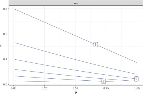
To investigate the sensitivity of ${\mathcal{R}}_c$ to coverage tracing probability p and the testing probability τ, we plot the control reproduction number as a function of p and τ in Figure 5. This contour plot shows that ${\mathcal{R}}_c$ decreases with both p and τ. In this figure, the level curves have a negative slope with a magnitude less than 1. This means that a small increase in τ has the same effect on ${\mathcal{R}}_c$ as a large increase in p. Thus, ${\mathcal{R}}_c$ is more sensitive to τ than to p. In addition, the magnitude of the slope increases as τ increases for each fixed p; thus, the sensitivity to p increases with τ. This is because more tests trigger more contact tracing, and thus make tracing more effective.

Figure 5. The contour plot of ${\mathcal{R}}_c$ as a function of the contact tracing coverage probability p and the testing rate τ. Here $\text{β}=0.4$, $\gamma =0.1$, $\theta =1$.

The dependence of ${\mathcal{R}}_c$ on the tracing rate θ and the transmission rate β is difficult to study analytically. We illustrate these dependencies using numerical simulations. Figure 6 illustrates that ${\mathcal{R}}_c$ is a decreasing function of θ, because $\theta v^{\ast }$ and $\theta w^{\ast }$ are increasing functions of θ. This is because increasing θ speeds up contact tracing, and thus more contacts are traced. 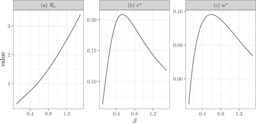Note that, as θ approaches ∞, $\theta v^{\ast }$, $\theta w^{\ast }$ and ${\mathcal{R}}_c$ have limits. Figure 7 shows that ${\mathcal{R}}_c$ is an increasing function of β. Interestingly, the average number of diagnosed infectors $v^{\ast }$ and the average number of diagnosed secondary infections $w^{\ast }$ are unimodal functions of β. The reason for this is not intuitive. We suspect that a moderate increase in β leads to more secondary infections, thus, increasing the average number of infectors and infectees that are diagnosed; while this increase also speeds up contact tracing and thus removes more infectors than infectees for very large β. Note that here, we use p = 1 to show that even if the contact tracing coverage is 1, ${\mathcal{R}}_c$ may still be above 1 when θ is small or when β is large.

Figure 6. The dependence of the control reproduction number ${\mathcal{R}}_c$, $\theta v^{\ast }$, and $\theta w^{\ast }$ on the tracing rate θ. Here $\gamma =0.1$, $\tau =0.15$, p = 1, $\text{β}=0.4$. Specifically, (b) reflects the contact tracing rate initiated from the infector and (c) reflects the rate initiated from an infectee. This figure also shows that contact tracing is more likely to originate from an infector as $\theta v^{\ast }>\theta w^{\ast }$.

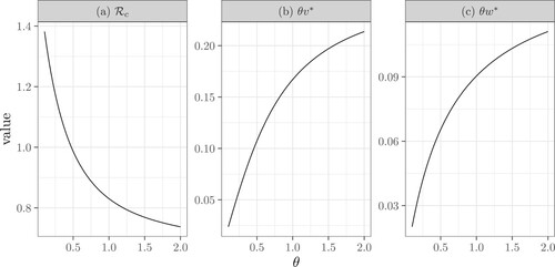
Figure 7. The dependence of the control reproduction number ${\mathcal{R}}_c$, the fraction of diagnosed infectors ($v^{\ast }$), and the average number of diagnosed secondary infections ($w^{\ast }$) on the transmission rate β. Here $\gamma =0.1$, $\tau =0.15$, p = 1, $\theta =1$.

5. The effect of tracing capacity on ${\mathcal{R}}_c$

In the compartmental SIR contact tracing model, the total contact tracing rate in the population is $\theta T$. When the diagnosed population T is large, the contact tracing capacity becomes a limiting factor. To understand the effect of contact tracing capacity on the effectiveness of contact tracing, we model the per capita contact tracing rate θ as a decreasing function of T, so that $\theta T$ is a saturating function of T. Specifically, (8) $\theta =\frac{{\theta }_0}{1+\frac{{\theta }_0}{{\theta }_{\mathrm{\infty }}}T},$(8) where ${\theta }_0$ is the per capita tracing rate with units 1/time when T is small, and ${\displaystyle {\theta }_{\mathrm{\infty }}=\underset{T\to \mathrm{\infty }}{lim}\theta T}$ is the tracing capacity with units person$/$time.

At the disease-free equilibrium, T = 0 and $\theta ={\theta }_0$, the control reproduction number defined in (6(6) ${\mathcal{R}}_c=\frac{\text{β}}{\gamma +\tau +\theta p(v^{\ast }+w^{\ast })}.$(6) ) becomes ${\mathcal{R}}_c=\frac{\text{β}}{\gamma +\tau +{\theta }_{0}p(v^{\ast }+w^{\ast })}.$On the other hand, as $T\to \mathrm{\infty }$, $\theta \to 0$, and ${\mathcal{R}}_c$ becomes ${\mathcal{R}}_0$ in (7(7) ${\mathcal{R}}_0=\frac{\text{β}}{\gamma +\tau }.$(7) ). 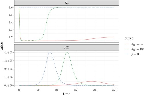Thus, when the number of diagnosed patients T is large so that the tracing reaches capacity, ${\mathcal{R}}_c$ becomes the same as without contact tracing. Figure 8 illustrates this effect. Note that the ${\mathcal{R}}_c$ starts as the basic reproduction number ${\mathcal{R}}_0$ because no patient has been diagnosed. Then ${\mathcal{R}}_c$ quickly reduces to the value given in Equation (6(6) ${\mathcal{R}}_c=\frac{\text{β}}{\gamma +\tau +\theta p(v^{\ast }+w^{\ast })}.$(6) ), and if contact tracing reaches capacity ${\mathcal{R}}_c$ increases and may approach ${\mathcal{R}}_0$ again. This may happen long before the epidemic reaches its peak. As well, we can see that the implementation of contact tracing delays the peak of the epidemic as shown in the comparison between the curves in both panels of Figure 8 where p = 0 (no contact tracing) and the tracing capacity ${\theta }_{\mathrm{\infty }}=100$. The most significant impact, however, is the inhibition of the growth of ${\mathcal{R}}_c$ and the associated delay and restriction of the epidemic peak when the tracing capacity ${\theta }_{\mathrm{\infty }}\to \mathrm{\infty }$.

Figure 8. The change in the control reproduction number (${\mathcal{R}}_c$, shown in the top panel), and the number of infectious individuals (I, shown in the bottom panel) as a function of time. The blue dashed curve with p = 0 reflects the case where contact tracing does not occur. Comparatively, the green dashed curve shows the case where: p = 0.4 and ${\theta }_{\mathrm{\infty }}=100$. Finally, the red curve shows the case where p = 0.3 and ${\theta }_{\mathrm{\infty }}=\mathrm{\infty }$. Here, the remaining fixed values and parameters are: $N=5\times {10}^6$, $\text{β}=0.4$, $\tau =0.15$, $\gamma =0.1$, ${\theta }_0=10$.

6. Concluding remarks

Our novel approach for modelling contact tracing of an infectious disease (Section 2) combines the convenience of a randomly mixed population with the precise tracking of the contacts in a network model. Thus to apply this model, detailed population contact information is not required.

Our analysis shows that the reproduction number ${\mathcal{R}}_c$ decreases as the contact tracing coverage probability p increases (Appendix 3). This is to be expected because as the fraction of individuals identified for testing and isolation increases, the remaining unidentified fraction of individuals that contribute to transmission decreases. We also find that when there is a large transmission rate β, contact tracing alone may not control the disease (Figure 7); thus, additional public health measures to decrease the transmission rate will need to be implemented in order for contact tracing to be effective. These findings are in alignment with other study results mentioned previously [6, 10, 12, 15, 22, 33]. We also find that ${\mathcal{R}}_c$ is more sensitive to the testing rate τ than to coverage probability p (Figure 5). Specifically, when testing rate is increased, ${\mathcal{R}}_c$ becomes more sensitive to the coverage probability. Thus, increasing testing coverage allows the effectiveness of contact tracing to also increase.

While this model only considers symptomatic infections and symptomatic testing, we can assess the impact of transmission from asymptomatic and pre-symptomatic infected individuals on the ability of contact tracing to effectively control the disease. When symptomatic testing is the primary method for identifying positive cases, this ultimately reduces the fraction of all infectious individuals (symptomatic, pre-symptomatic, and asymptomatic) who are tested, diagnosed, and isolated. This is represented by a reduced testing rate τ, which thereby decreases the contact tracing coverage p. Thus, the reduction of the fraction of individuals tested reduces the effectiveness of contact tracing. This finding was also reported in [12].

We also show that at the initial phase of the epidemic and thus when T is small, contact tracing can reduce ${\mathcal{R}}_c$, and this also agrees with [12]. However, as T increases and becomes large, contact tracing becomes saturated due to limited resources to effectively trace all contacts following positive diagnosis (keeping all other parameters fixed). Thus, ${\mathcal{R}}_c$ quickly increases back to ${\mathcal{R}}_0$ (Figure 8). Note that this only occurs when tracing capacity ${\theta }_{\mathrm{\infty }}\ll \mathrm{\infty }$, and this reversal may occur much earlier than the actual epidemic peak. Overall, contact tracing is most effective during the initial exponential growth phase of the epidemic in all scenarios. We show that when all other parameters remained fixed, (i.e. no additional interventions applied to reduce the transmission rate β) and ${\theta }_{\mathrm{\infty }}\ll \mathrm{\infty }$, contact tracing reaches capacity and has limited effectiveness prior to the main peak of the epidemic. However, when the tracing capacity ${\theta }_{\mathrm{\infty }}$ approaches ∞, the epidemic peak is not only delayed, but significantly suppressed. Note that these results implicitly assume a positive diagnosis rate, i.e. $\tau >0$.

As this is a simple SIR model that has been extended to include both testing and contact tracing, it does not accurately reflect the reality of many infectious diseases that do have pre-symptomatic or asymptomatic transmission. However, this model can be extended to incorporate exposed, asymptomatic, and pre-symptomatic compartments as well as differing testing and isolation policies. With these extensions, this model may be fit to case count data to estimate the contact tracing coverage p and other parameters, and these parameter values used to evaluate the effect of contact tracing on the control reproduction number and epidemic final size. Further, the implementation of non-pharmaceutical interventions, vaccination, and treatment measures can also be included in the model. It is not clear how these extensions would affect our conclusions if incorporated; this is left for future work. In the case of SARS-CoV-2, the differences in variant transmissibility and detection should also be considered with regard to contact tracing effectiveness. Because saturation of contact tracing and testing capacity and resources have been shown to impact the effectiveness of contact tracing activities, it would be useful to incorporate cost–benefit and cost-effectiveness analyses to this model to help further inform public health interventions and policies in responding to current and future epidemics of concern. It may be that if resources for contact tracing become scarce, public health should shift to more effective mitigation strategies.

Acknowledgments

We thank the anonymous reviewers for their constructive comments and suggestions.

Disclosure statement

No potential conflict of interest was reported by the authors.

Additional information

Funding

This research is funded by: Michael Smith Foundation for Health Research and the Victoria Hospitals Foundation (LC), Canadian Institutes for Health Research (JM), Natural Sciences and Engineering Research Council (NSERC) Discovery Grants (LC, JM, PvdD), and NSERC Undergraduate Student Research Award (SB).

Appendices

Appendix 1. Flowchart of the full pair dynamics

The flowchart in Figure 3 includes only the dynamics of the pairs $[I\leftarrow I]$, $[I\leftarrow T]$ and $[T\leftarrow I]$. The pairs $[I\leftarrow X]$, $[I\leftarrow R]$, $[T\leftarrow T]$, $[T\leftarrow X]$ and $[T\leftarrow R]$ are not tracked in that flowchart, even though they are valid states. In Figure A1, we give the full flowchart for all these pairs. The equations in (1a(1a) $\begin{array}{rl}{S}^{\prime }& =-\text{β}S\frac{I}{N},\end{array}$(1a) ) can be read from this flowchart with the relationships $I=[I\leftarrow I]+[I\leftarrow T]+[I\leftarrow X]+[I\leftarrow R]$ and $T=[T\leftarrow I]+[T\leftarrow T]+[T\leftarrow X]+[T\leftarrow R]$.

Figure A1. The full flowchart of the pair dynamics for Model (1a(1a) $\begin{array}{rl}{S}^{\prime }& =-\text{β}S\frac{I}{N},\end{array}$(1a) )-(1h).

Appendix 2

Uniqueness and stability of disease-free equilibrium

Here we show that the system (2a(2a) $\begin{array}{rl}{S}^{\prime }& =\text{β}S\frac{I}{N}\end{array}$(2a) )-(2e) has a unique biologically meaningful disease-free equilibrium (DFE) that is globally asymptotically stable in the disease-free invariant set $\mathcal{H}$.

Equation (4(4) $G\left(w^{\ast }\right):=(\text{β}+\theta )\theta p{w}^{\ast 2}+\left[\right(\text{β}+\theta \left)\right(\text{β}+\tau +\gamma )-\text{β}\theta p]w^{\ast }-\text{β}\tau =0.$(4) ) gives a unique positive root $w^{\ast }$. We will show that equation (5(5) $F\left(v^{\ast }\right):=\theta p{v}^{\ast 2}+(\theta p{u}^{\ast }-\text{β}-\theta )v^{\ast }+\theta p{u}^{\ast }{w}^{\ast }+\tau u^{\ast }=0.$(5) ) has two positive roots, and only one is in the invariant region $\mathcal{H}$ (i.e. biologically meaningful). This is true if (A1) $F(1-u^{\ast })=\tau u^{\ast }+\theta p{u}^{\ast }{w}^{\ast }+(\theta p{u}^{\ast }-\text{β}-\theta )(1-u^{\ast })+\theta p(1-u^{\ast }{)}^2<0,$(A1) and thus the larger root satisfies $v^{\ast }>1-u^{\ast }$ and is outside of $\mathcal{H}$, while the smaller root satisfies $v^{\ast }<1-u^{\ast }$ and is inside $\mathcal{H}$. To show that (A1(A1) $F(1-u^{\ast })=\tau u^{\ast }+\theta p{u}^{\ast }{w}^{\ast }+(\theta p{u}^{\ast }-\text{β}-\theta )(1-u^{\ast })+\theta p(1-u^{\ast }{)}^2<0,$(A1) ) is true, note that from (2e(2e) $\begin{array}{rl}{w}^{\prime }& =\tau u-(\text{β}+\theta )w+\theta puw.\end{array}$(2e) ), $\tau u^{\ast }+\theta p{u}^{\ast }{w}^{\ast }=(\text{β}+\theta )w^{\ast }.$In addition, adding (2c(2c) $\begin{array}{rl}{u}^{\prime }& =\text{β}\frac{S}{N}(1-u)-(\tau +\gamma )u-\theta puw,\end{array}$(2c) ) and (2e(2e) $\begin{array}{rl}{w}^{\prime }& =\tau u-(\text{β}+\theta )w+\theta puw.\end{array}$(2e) ) gives, $\text{β}-\text{β}{u}^{\ast }-\gamma u^{\ast }=(\text{β}+\theta )w^{\ast }.$The above two equations give (A2) $\tau u^{\ast }+\theta p{u}^{\ast }{w}^{\ast }=\text{β}-\text{β}{u}^{\ast }-\gamma u^{\ast }.$(A2) Thus, $\begin{array}{rl}F(1-u^{\ast })& =\text{β}-\text{β}{u}^{\ast }-\gamma u^{\ast }+\theta p(1-u^{\ast })-(\text{β}+\theta )(1-u^{\ast }),\\ & =-\gamma u^{\ast }-\theta (1-p)(1-u^{\ast })<0.\end{array}$This implies that there is a unique biologically meaningful disease-free equilibrium $(N,0,u^{\ast },v^{\ast },w^{\ast })$ in $\mathcal{H}$.

To study the stability of the DFE, we linearize this model about the DFE $(N,0,u^{\ast },v^{\ast },w^{\ast })$, and restrict to the invariant set $\mathcal{H}$. The dynamics of the linearized system is only determined by the equations of I, u, v and w. From (2c(2c) $\begin{array}{rl}{u}^{\prime }& =\text{β}\frac{S}{N}(1-u)-(\tau +\gamma )u-\theta puw,\end{array}$(2c) )–(2e(2e) $\begin{array}{rl}{w}^{\prime }& =\tau u-(\text{β}+\theta )w+\theta puw.\end{array}$(2e) ), (A3a) $\begin{array}{rl}{u}^{\prime }& =\text{β}-\text{β}u-(\tau +\gamma )u-\theta puw:=f(u,w),\end{array}$(A3a) (A3b) $\begin{array}{rl}{v}^{\prime }& =\tau u+\theta pu(v+w)-(\text{β}+\theta )v+\theta p{v}^2,\end{array}$(A3b) (A3c) $\begin{array}{rl}{w}^{\prime }& =\tau u-(\text{β}+\theta )w+\theta puw:=g(u,w).\end{array}$(A3c) Note that u and w are independent of v. We thus first study (A3a(A3a) $\begin{array}{rl}{u}^{\prime }& =\text{β}-\text{β}u-(\tau +\gamma )u-\theta puw:=f(u,w),\end{array}$(A3a) ) and (A3c(A3c) $\begin{array}{rl}{w}^{\prime }& =\tau u-(\text{β}+\theta )w+\theta puw:=g(u,w).\end{array}$(A3c) ). At the positive equilibrium point $(u^{\ast },w^{\ast })$ where $0\le u^{\ast }\le 1$, the Jacobian of the $(u,w)$ system is $J=\left[\begin{array}{cc}-(\text{β}+\tau +\gamma +\theta p{w}^{\ast })& -\theta p{u}^{\ast }\\ \tau +\theta p{w}^{\ast }& \theta p{u}^{\ast }-(\text{β}+\theta )\end{array}\right].$The trace $tr\left(J\right)=-(\text{β}+\tau +\gamma +\theta p{w}^{\ast })+\theta p{u}^{\ast }-(\text{β}+\theta )<0,$and the determinant $det\left(J\right)=(\text{β}+\theta )(\text{β}+\tau +\gamma +\theta p{w}^{\ast })-(\text{β}+\gamma )\theta p{u}^{\ast }>0.$Hence, this DFE is locally asymptotically stable.

We use the Bendixon criterion to show the global stability of the DFE. Because $p\le 1$ and $u\le 1$, $\frac{\mathrm{\partial }f}{\mathrm{\partial }u}+\frac{\mathrm{\partial }g}{\mathrm{\partial }w}=-(\text{β}+\tau +\gamma +\theta pw)-(\text{β}+\theta )+\theta pu<0,$and thus the $(u,w)$ system has no periodic solution in the invariant set $\mathcal{H}$. Thus, in $\mathcal{H}$, all solutions satisfy $u\left(t\right)\to u^{\ast }$ and $w\left(t\right)\to w^{\ast }$ as $t\to \mathrm{\infty }$. To study the behaviour of $v\left(t\right)$, substitute $(u^{\ast },w^{\ast })$ into the equation for v: $v^{\prime }=\tau u^{\ast }+\theta p{u}^{\ast }{w}^{\ast }+(\theta p{u}^{\ast }-\text{β}-\theta )v+\theta p{v}^2.$Note that $v^{\ast }$ is the smaller root of $F\left(v\right)=0$, $F^{\prime }\left(v^{\ast }\right)<0$, and thus $v^{\ast }$ is locally asymptotically stable. Because this is a one-dimensional autonomous equation, all solutions in the invariant set $\mathcal{H}$ approach the biologically meaningful DFE $(N,0,u^{\ast },v^{\ast },w^{\ast })$.

Appendix 3

The dependence of ${\mathcal{R}}_c$ on p and τ

Here we prove that ${\mathcal{R}}_c$ is a decreasing function of the tracing coverage p and the testing rate τ. To show the dependence on p, we calculate $\mathrm{\partial }{w}^{\ast }/\mathrm{\partial }p$ from equation (4(4) $G\left(w^{\ast }\right):=(\text{β}+\theta )\theta p{w}^{\ast 2}+\left[\right(\text{β}+\theta \left)\right(\text{β}+\tau +\gamma )-\text{β}\theta p]w^{\ast }-\text{β}\tau =0.$(4) ). $\frac{\mathrm{\partial }{w}^{\ast }}{\mathrm{\partial }p}=-\frac{\mathrm{\partial }G/\mathrm{\partial }p}{\mathrm{\partial }G/\mathrm{\partial }{w}^{\ast }},$where $\mathrm{\partial }G/\mathrm{\partial }p=(\text{β}+\theta )\theta w^{\ast }(w^{\ast }-\frac{\text{β}}{\text{β}+\theta }),$and $\mathrm{\partial }G/\mathrm{\partial }{w}^{\ast }>0$ (because G has a positive root and a negative root, thus $w^{\ast }$ is the larger root of (4(4) $G\left(w^{\ast }\right):=(\text{β}+\theta )\theta p{w}^{\ast 2}+\left[\right(\text{β}+\theta \left)\right(\text{β}+\tau +\gamma )-\text{β}\theta p]w^{\ast }-\text{β}\tau =0.$(4) )). To determine the sign of $\mathrm{\partial }G/\mathrm{\partial }p$, we need to calculate the sign of $w^{\ast }-\frac{\text{β}}{\text{β}+\theta }$. Consider $\begin{array}{rl}G\left(\frac{\text{β}}{\text{β}+\theta }\right)& =(\text{β}+\theta )\theta p{\left(\frac{\text{β}}{\text{β}+\theta }\right)}^2+\left[\right(\text{β}+\theta \left)\right(\text{β}+\tau +\gamma )-\text{β}\theta p]\frac{\text{β}}{\text{β}+\theta }-\text{β}\tau \\ & =\text{β}(\text{β}+\gamma )>0,\end{array}$and ${\frac{\mathrm{\partial }G}{\mathrm{\partial }{w}^{\ast }}|}_{\frac{\text{β}}{\text{β}+\theta }}=\theta p\text{β}+(\text{β}+\theta )(\text{β}+\tau +\gamma )>0.$Thus, $\text{β}/(\text{β}+\theta )>w^{\ast }$. Hence, $\mathrm{\partial }G/\mathrm{\partial }p<0$, giving $\frac{\mathrm{\partial }{w}^{\ast }}{\mathrm{\partial }p}>0,$ therefore, the value of $w^{\ast }$ increases as p increases.

Similarly, we calculate $\mathrm{\partial }{v}^{\ast }/\mathrm{\partial }p$ from (5(5) $F\left(v^{\ast }\right):=\theta p{v}^{\ast 2}+(\theta p{u}^{\ast }-\text{β}-\theta )v^{\ast }+\theta p{u}^{\ast }{w}^{\ast }+\tau u^{\ast }=0.$(5) ). Equation (A3c(A3c) $\begin{array}{rl}{w}^{\prime }& =\tau u-(\text{β}+\theta )w+\theta puw:=g(u,w).\end{array}$(A3c) ) gives $\theta p{u}^{\ast }{w}^{\ast }+\tau u^{\ast }=(\text{β}+\theta )w^{\ast }.$Substituting this into (5(5) $F\left(v^{\ast }\right):=\theta p{v}^{\ast 2}+(\theta p{u}^{\ast }-\text{β}-\theta )v^{\ast }+\theta p{u}^{\ast }{w}^{\ast }+\tau u^{\ast }=0.$(5) ) gives (A4) $F=\theta p{v}^{\ast 2}+(\theta p{u}^{\ast }-\text{β}-\theta )v^{\ast }+(\text{β}+\theta )w^{\ast }=0.$(A4) Thus, taking the total derivative of F gives $\frac{\mathrm{\partial }{v}^{\ast }}{\mathrm{\partial }p}=-\frac{\frac{\mathrm{\partial }F}{\mathrm{\partial }{u}^{\ast }}\frac{\mathrm{\partial }{u}^{\ast }}{\mathrm{\partial }p}+\frac{\mathrm{\partial }F}{\mathrm{\partial }{w}^{\ast }}\frac{\mathrm{\partial }{w}^{\ast }}{\mathrm{\partial }p}+\frac{\mathrm{\partial }F}{\mathrm{\partial }p}}{\mathrm{\partial }F/\mathrm{\partial }{v}^{\ast }}.$Here, $\frac{\mathrm{\partial }F}{\mathrm{\partial }p}=\theta (v^{\ast }{)}^2+\theta u^{\ast }{v}^{\ast },\frac{\mathrm{\partial }F}{\mathrm{\partial }{u}^{\ast }}=\theta p{v}^{\ast },\frac{\mathrm{\partial }F}{\mathrm{\partial }{w}^{\ast }}=\text{β}+\theta ,$and $\mathrm{\partial }F/\mathrm{\partial }{v}^{\ast }<0$ (because $v^{\ast }$ is the smaller root of (A4(A4) $F=\theta p{v}^{\ast 2}+(\theta p{u}^{\ast }-\text{β}-\theta )v^{\ast }+(\text{β}+\theta )w^{\ast }=0.$(A4) )). The sign of $\mathrm{\partial }{v}^{\ast }/\mathrm{\partial }p$ is determined by the sign of its numerator. From (3(3) $u^{\ast }=\frac{\text{β}}{\text{β}+\tau +\gamma +\theta p{w}^{\ast }},$(3) ), $\begin{array}{rl}\frac{\mathrm{\partial }{u}^{\ast }}{\mathrm{\partial }p}& =-\frac{\text{β}\theta p}{(\text{β}+\tau +\gamma +\theta p{w}^{\ast }{)}^2}\frac{\mathrm{\partial }{w}^{\ast }}{\mathrm{\partial }p}-\frac{\text{β}\theta w^{\ast }}{(\text{β}+\tau +\gamma +\theta p{w}^{\ast }{)}^2}\\ & =-\frac{\theta p{u}^{\ast }}{\text{β}+\tau +\gamma +\theta p{w}^{\ast }}\frac{\mathrm{\partial }{w}^{\ast }}{\mathrm{\partial }p}-\frac{\theta w^{\ast }{u}^{\ast }}{\text{β}+\tau +\gamma +\theta p{w}^{\ast }}.\end{array}$Thus, $\begin{array}{rl}& \frac{\mathrm{\partial }F}{\mathrm{\partial }{u}^{\ast }}\frac{\mathrm{\partial }{u}^{\ast }}{\mathrm{\partial }p}+\frac{\mathrm{\partial }F}{\mathrm{\partial }{w}^{\ast }}\frac{\mathrm{\partial }{w}^{\ast }}{\mathrm{\partial }p}+\frac{\mathrm{\partial }F}{\mathrm{\partial }p}=-\frac{(\theta p{)}^2{v}^{\ast }{u}^{\ast }}{\text{β}+\tau +\gamma +\theta p{w}^{\ast }}\frac{\mathrm{\partial }{w}^{\ast }}{\mathrm{\partial }p}-\frac{{\theta }^{2}p{v}^{\ast }{w}^{\ast }{u}^{\ast }}{\text{β}+\tau +\gamma +\theta p{w}^{\ast }}\\ & +(\text{β}+\theta )\frac{\mathrm{\partial }{w}^{\ast }}{\mathrm{\partial }p}+\theta (v^{\ast }{)}^2+\theta u^{\ast }{v}^{\ast }.\end{array}$Note that, (A5) $-\frac{(\theta p{)}^2{v}^{\ast }{u}^{\ast }}{\text{β}+\tau +\gamma +\theta p{w}^{\ast }}\frac{\mathrm{\partial }{w}^{\ast }}{\mathrm{\partial }p}+\theta \frac{\mathrm{\partial }{w}^{\ast }}{\mathrm{\partial }p}=\frac{\text{β}+\tau +\gamma +\theta p{w}^{\ast }-\theta p^2{u}^{\ast }{v}^{\ast }}{\text{β}+\tau +\gamma +\theta p{w}^{\ast }}\theta \frac{\mathrm{\partial }{w}^{\ast }}{\mathrm{\partial }p}>0$(A5) in the case of ${\mathcal{R}}_c>1$, i.e. $\text{β}>\gamma +\tau +\theta p(u^{\ast }+v^{\ast })$. In addition, $\frac{{\theta }^{2}p{u}^{\ast }{v}^{\ast }{w}^{\ast }}{\text{β}+\tau +\gamma +\theta p{w}^{\ast }}\le \theta u^{\ast }{v}^{\ast },$and thus $\frac{\mathrm{\partial }F}{\mathrm{\partial }{u}^{\ast }}\frac{\mathrm{\partial }{u}^{\ast }}{\mathrm{\partial }p}+\frac{\mathrm{\partial }F}{\mathrm{\partial }{w}^{\ast }}\frac{\mathrm{\partial }{w}^{\ast }}{\mathrm{\partial }p}+\frac{\mathrm{\partial }F}{\mathrm{\partial }p}>0.$This gives $\mathrm{\partial }{v}^{\ast }/\mathrm{\partial }p>0$. Therefore, if ${\mathcal{R}}_c>1$, both $v^{\ast }$ and $w^{\ast }$ are increasing functions of p. Thus, $\frac{\mathrm{\partial }{\mathcal{R}}_c}{\mathrm{\partial }p}<0.$We use a similar approach to prove that ${\mathcal{R}}_c$ is a decreasing function of τ for $R_c>1$. From Equation (4(4) $G\left(w^{\ast }\right):=(\text{β}+\theta )\theta p{w}^{\ast 2}+\left[\right(\text{β}+\theta \left)\right(\text{β}+\tau +\gamma )-\text{β}\theta p]w^{\ast }-\text{β}\tau =0.$(4) ), $\frac{\mathrm{\partial }{w}^{\ast }}{\mathrm{\partial }\tau }=-\frac{\mathrm{\partial }G/\mathrm{\partial }\tau }{\mathrm{\partial }G/\mathrm{\partial }{w}^{\ast }},$where $\mathrm{\partial }G/\mathrm{\partial }\tau =(\text{β}+\theta )w^{\ast }-\text{β},$and $\mathrm{\partial }G/\mathrm{\partial }{w}^{\ast }>0$. Because $\text{β}/(\text{β}+\theta )>w^{\ast }$, $\mathrm{\partial }G/\mathrm{\partial }\tau <0$. Thus, $\frac{\mathrm{\partial }{w}^{\ast }}{\mathrm{\partial }\tau }=-\frac{\mathrm{\partial }G/\mathrm{\partial }\tau }{\mathrm{\partial }G/\mathrm{\partial }{w}^{\ast }}>0.$To calculate $\mathrm{\partial }{v}^{\ast }/\mathrm{\partial }p$, we rewrite (5(5) $F\left(v^{\ast }\right):=\theta p{v}^{\ast 2}+(\theta p{u}^{\ast }-\text{β}-\theta )v^{\ast }+\theta p{u}^{\ast }{w}^{\ast }+\tau u^{\ast }=0.$(5) ). From (A2(A2) $\tau u^{\ast }+\theta p{u}^{\ast }{w}^{\ast }=\text{β}-\text{β}{u}^{\ast }-\gamma u^{\ast }.$(A2) ), $F=\theta p{v}^{\ast 2}+(\theta p{u}^{\ast }-\text{β}-\theta )v^{\ast }+\text{β}-\text{β}{u}^{\ast }-\gamma u^{\ast }=0.$Thus, $\frac{\mathrm{\partial }{v}^{\ast }}{\mathrm{\partial }\tau }=-\frac{\frac{\mathrm{\partial }F}{\mathrm{\partial }{u}^{\ast }}\frac{\mathrm{\partial }{u}^{\ast }}{\mathrm{\partial }\tau }}{\mathrm{\partial }F/\mathrm{\partial }{v}^{\ast }}.$Here, $\frac{\mathrm{\partial }F}{\mathrm{\partial }{u}^{\ast }}=\theta p{v}^{\ast }-\text{β}-\gamma ,\mathrm{\partial }F/\mathrm{\partial }{v}^{\ast }<0.$To determine the sign of $\mathrm{\partial }{v}^{\ast }/\mathrm{\partial }\tau$, we calculate the sign of its numerator. From (3(3) $u^{\ast }=\frac{\text{β}}{\text{β}+\tau +\gamma +\theta p{w}^{\ast }},$(3) ), $\begin{array}{rl}\frac{\mathrm{\partial }{u}^{\ast }}{\mathrm{\partial }\tau }& =-\frac{\text{β}\theta p}{(\text{β}+\tau +\gamma +\theta p{w}^{\ast }{)}^2}\frac{\mathrm{\partial }{w}^{\ast }}{\mathrm{\partial }\tau }-\frac{\text{β}}{(\text{β}+\tau +\gamma +\theta p{w}^{\ast }{)}^2}\\ & =-\frac{\theta p{u}^{\ast }}{\text{β}+\tau +\gamma +\theta p{w}^{\ast }}\frac{\mathrm{\partial }{w}^{\ast }}{\mathrm{\partial }\tau }-\frac{u^{\ast }}{\text{β}+\tau +\gamma +\theta p{w}^{\ast }}.\end{array}$Thus, $\frac{\mathrm{\partial }F}{\mathrm{\partial }{u}^{\ast }}\frac{\mathrm{\partial }{u}^{\ast }}{\mathrm{\partial }\tau }=(\text{β}+\gamma -\theta p{v}^{\ast })[\frac{\theta p{u}^{\ast }}{\text{β}+\tau +\gamma +\theta p{w}^{\ast }}\frac{\mathrm{\partial }{w}^{\ast }}{\mathrm{\partial }\tau }+\frac{u^{\ast }}{\text{β}+\tau +\gamma +\theta p{w}^{\ast }}].$In the case of ${\mathcal{R}}_c>1$ ( i.e. $\text{β}>\gamma +\tau +\theta p(u^{\ast }+v^{\ast })$), $\frac{\mathrm{\partial }F}{\mathrm{\partial }{u}^{\ast }}\frac{\mathrm{\partial }{u}^{\ast }}{\mathrm{\partial }\tau }>0.$Thus, $\frac{\mathrm{\partial }{v}^{\ast }}{\mathrm{\partial }\tau }>0$. Hence, if ${\mathcal{R}}_c>1$, $v^{\ast }$ and $w^{\ast }$ are increasing functions of τ. Thus $\frac{\mathrm{\partial }{\mathcal{R}}_c}{\mathrm{\partial }\tau }<0.$

References

- G.M. Ames, D.B. George, C.P. Hampson, A.R. Kanarek, C.D. McBee, and D.R. Lockwood, et al. Using network properties to predict disease dynamics on human contact networks, Proc. Biol. Sci. 278(1724) (2011), pp. 3544–3550. Available at https://www.ncbi.nlm.nih.gov/pmc/articles/PMC3189367/.
- F. Brauer, Compartmental Models in Epidemiology, in Mathematical Epidemiology, Mathematical Biosciences Subseries. Springer, 2008, pp. 19–78.
- Canadian Broadcasting Corporation (CBC), B.C.'s contact tracing and testing at maximum capacity, health officials say | CBC News; 2021. Available at https://www.cbc.ca/news/canada/british-columbia/covid-briefing-dec24-1.6297668.
- Centers for Disease Control and Prevention (CDC), CDC Diagnostic Tests for COVID-19; 2021. Available at https://www.cdc.gov/coronavirus/2019-ncov/lab/testing.html.
- A. Fontanet, B. Autran, B. Lina, M.P. Kieny, S.S.A. Karim, and D. Sridhar, SARS-CoV-2 variants and ending the COVID-19 pandemic, Lancet 397(10278) (2021), pp. 952–954.
- C. Fraser, S. Riley, R.M. Anderson, and N.M. Ferguson, Factors that make an infectious disease outbreak controllable, Proc. Natl. Acad. Sci. U.S.A. 101(16) (2004), pp. 6146–6151. Available at https://www.ncbi.nlm.nih.gov/pmc/articles/PMC395937/.
- D.M. Green and I.Z. Kiss, Large-scale properties of clustered networks: Implications for disease dynamics, J. Biol. Dynam. 4(5) (2010), pp. 431–445. doi: 10.1080/17513758.2010.487158.
- A.B. Gumel, E.A. Iboi, C.N. Ngonghala, and E.H. Elbasha, A primer on using mathematics to understand COVID-19 dynamics: Modeling, analysis and simulations, Infect. Dis. Model. 6 (2020), pp. 148–168. Available at https://www.ncbi.nlm.nih.gov/pmc/articles/PMC7786036/.
- D.J. Haw, R. Pung, J.M. Read, and S. Riley, Strong spatial embedding of social networks generates nonstandard epidemic dynamics independent of degree distribution and clustering, Proc. Natl. Acad. Sci. 117(38) (2020), pp. 23636–23642. doi: 10.1073/pnas.1910181117.
- J. Hellewell, S. Abbott, A. Gimma, N.I. Bosse, C.I. Jarvis, and T.W. Russell, et al. Feasibility of controlling COVID-19 outbreaks by isolation of cases and contacts, Lancet. Glob. Health. 8(4) (2020), pp. e488–e496. Available at https://linkinghub.elsevier.com/retrieve/pii/S2214109X20300747.
- R. Huerta and L.S. Tsimring, Contact tracing and epidemics control in social networks, Phys. Rev. E. 66(5) (2002), pp. 056115. doi: 10.1103/PhysRevE.66.056115.
- M.A. Johansson, T.M. Quandelacy, S. Kada, P.V. Prasad, M. Steele, and J.T. Brooks, et al. SARS-CoV-2 transmission from people without COVID-19 symptoms, JAMA Netw. Open. 4(1) (2021), pp. e2035057.doi: 10.1001/jamanetworkopen.2020.35057.
- M.J. Keeling, The effects of local spatial structure on epidemiological invasions, Proc. Biol. Sci. 266(1421) (1999), pp. 859–867. Available at https://www.ncbi.nlm.nih.gov/pmc/articles/PMC1689913/.
- M.J. Keeling and D.A. Rand, Spatial correlations and local fluctuations in host-parasite models, in From Finite to Infinite Dimensional Dynamical Systems, J. Robinson and P. A. Glendinning, eds., Springer, 2001, pp. 5–57.
- M.E. Kretzschmar, G. Rozhnova, and M. van Boven, Isolation and contact tracing can tip the scale to containment of COVID-19 in populations with social distancing, Front. Phys. 8 (2021). doi: 10.3389/fphy.2020.622485.
- K.O. Kwok, A. Tang, V.W.I. Wei, W.H. Park, E.K. Yeoh, and S. Riley, Epidemic models of contact tracing: systematic review of transmission studies of severe acute respiratory syndrome and Middle East respiratory syndrome, Comput. Struct. Biotechnol. J. 17 (2019), pp. 186–194. Available at https://www.sciencedirect.com/science/article/pii/S2001037018301703.
- A. Lambert, A mathematical assessment of the efficiency of quarantining and contact tracing in curbing the COVID-19 epidemic, Math. Model. Nat. Phenom. 16 (2021), pp. 53. Available at https://www.mmnp-journal.org/articles/mmnp/abs/2021/01/mmnp200298/mmnp200298.html.
- M. Lipsitch, T. Cohen, and B. Cooper, et al. Transmission dynamics and control of severe acute respiratory syndrome, Science 300 (5627) (2003), pp. 1966–1970.
- D. Lunz, G. Batt, and J. Ruess, To quarantine, or not to quarantine: A theoretical framework for disease control via contact tracing, Epidemics 34 (2021), pp. 100428. Available at https://www.sciencedirect.com/science/article/pii/S1755436520300475.
- J.C. Miller, Percolation and epidemics in random clustered networks, Phys. Rev. E. 80(2) (2009), pp. 020901. doi: 10.1103/PhysRevE.80.020901
- I. Nåsell, The quasi-stationary distribution of the closed endemic sis model, Adv. Appl. Prob. 28(3) (1996), pp. 895–932. Available at https://www.cambridge.org/core/journals/advances-in-applied-probability/article/abs/quasistationary-distribution-of-the-closed-endemic-sis-model/C2EAD1B7436261EC9336216592D2C31A.
- B. Nussbaumer-Streit, V. Mayr, A.I. Dobrescu, A. Chapman, E. Persad, and I. Klerings, et al. Quarantine alone or in combination with other public health measures to control COVID?19: A rapid review, Cochrane Database Syst. Rev. 2020(9) (2020), pp. CD013574. Available at https://www.ncbi.nlm.nih.gov/pmc/articles/PMC8133397/.
- S.P. Otto, T. Day, J. Arino, C. Colijn, J. Dushoff, and M. Li, et al. The origins and potential future of SARS-CoV-2 variants of concern in the evolving COVID-19 pandemic, Curr. Biol. 31(14) (2021), pp. R918–R929. Available at https://www.ncbi.nlm.nih.gov/pmc/articles/PMC8220957/.
- C.E. Overton, H.B.Stage, S. Ahmad, J. Curran-Sebastian, P. Dark, and R. Das, et al. Using statistics and mathematical modelling to understand infectious disease outbreaks: COVID-19 as an example, Infect. Dis. Model. 5 (2020), pp. 409–441. Available at https://www.ncbi.nlm.nih.gov/pmc/articles/PMC7334973/.
- M.S. Shkarayev, I. Tunc, and L.B. Shaw, Epidemics with temporary link deactivation in scale-free networks, J. Phys. A. Math. Theor. 47(45) (2014), pp. 455006. Available at https://www.ncbi.nlm.nih.gov/pmc/articles/PMC4238289/.
- S. Sturniolo, W. Waites, T. Colbourn, D. Manheim, and J. Panovska-Griffiths, Testing, tracing and isolation in compartmental models, PLOS. Comput. Biol. 17(3) (2021), pp. e1008633. doi: 10.1371/journal.pcbi.1008633.
- K.C. Swanson, C. Altare, C.S. Wesseh, T. Nyenswah, T. Ahmed, and N. Eyal, et al. Contact tracing performance during the ebola epidemic in Liberia, 2014-2015, PLOS. Neglect. Trop. D. 12(9) (2018), pp. e0006762. doi: 10.1371/journal.pntd.0006762.
- T.K. Tsang, P. Wu, Y. Lin, E.H.Y. Lau, G.M. Leung, and B.J. Cowling, Effect of changing case definitions for COVID-19 on the epidemic curve and transmission parameters in Mainland China: A modelling study, Lancet. Publ. Health. 5(5) (2020), pp. e289–e296. Available at https://www.thelancet.com/journals/lanpub/article/PIIS2468-2667(20)30089-X/fulltext.
- I. Tunc, L. Shaw, and M. Shkarayev, Epidemics in adaptive social networks with temporary link deactivation, J. Stat. Phys. 151(1-2) (2013), pp. 355–366. Available at https://scholarworks.wm.edu/aspubs/1669.
- E. Volz, SIR dynamics in random networks with heterogeneous connectivity, J. Math. Biol. 56(3) (2008), pp. 293–310. Available at https://pubmed.ncbi.nlm.nih.gov/17668212/.
- H.J. Wearing, P. Rohani, and M.J. Keeling, Appropriate models for the management of infectious diseases, PLoS. Med. 2 (7) (2005), pp. e174.
- World Health Organization (WHO), Coronavirus disease 2019 (COVID-19) – Situation Report -73; 2020. Available at https://apps.who.int/iris/bitstream/handle/10665/331686/nCoVsitrep02Apr2020-eng.pdf?sequence=1&isAllowed=y.
- J. Wu, B. Tang, N.L. Bragazzi, K. Nah, and Z. McCarthy, Quantifying the role of social distancing, personal protection and case detection in mitigating COVID-19 outbreak in Ontario, Canada, J. Math. Ind. 10(1) (2020), pp. 15. Available at https://www.ncbi.nlm.nih.gov/pmc/articles/PMC7249976/.
- R.A. Zayed, D. Omran, and A.A. Zayed, COVID-19 clinical and laboratory diagnosis overview, J. Egypt. Public Health Assoc. 96(1) (2021), pp. 25. doi: 10.1186/s42506-021-00087-w.