The effects of evolution on the stability of competing species

Abstract

Based on evolutionary game theory and Darwinian evolution, we propose and study discrete-time competition models of two species where at least one species has an evolving trait that affects their intra-specific, but not their inter-specific competition coefficients. By using perturbation theory, and the theory of the limiting equations of non-autonomous discrete dynamical systems, we obtain global stability results. Our theoretical results indicate that evolution may promote and/or suppress the stability of the coexistence equilibrium depending on the environment. This relies crucially on the speed of evolution and on how the intra-specific competition coefficient depends on the evolving trait. In general, equilibrium destabilization occurs when $\alpha >2$, when the speed of evolution is sufficiently slow. In this case, we conclude that evolution selects against complex dynamics. However, when evolution proceeds at a faster pace, destabilization can occur when $\alpha <2$. In this case, if the competition coefficient is highly sensitive to changes in the trait v, destabilization and complex dynamics occur. Moreover, destabilization may lead to either a period-doubling bifurcation, as in the non-evolutionary Ricker equation, or to a Neimark-Sacker bifurcation.

Keywords:

• Competition models
• evolutionary dynamics
• traits
• local stability
• asymptotically autonomous
• global stability

1. Introduction

Evolution is the physical, genetic, or behavioural change in populations of biological organisms over time. Evolution's more significant manifestations result from natural selection, a process that engineers biological systems. Understanding an evolutionary design has its roots in Darwin's three postulates (Darwin [12], Sober [28]). According to Lewontin [15], these postulates are:

• Postulate 1 (Variability). Like tends to beget like, and there is heritable variation in traits associated with each type of organism,

• Postulate 2 (Differential fitness). Among organisms, there is a struggle for existence,

• Postulate 3 (Heritability). Heritable traits influence the struggle for existence.

The strategy/postulate that there is a struggle for existence among organisms may be simulated using population dynamics models. Such models contain many parameters, such as growth rates, resources uptake rates, predation rates, and carrying capacities. These parameters, in turn, depend on the strategies (i.e. heritable traits) used by various species in the population.

Based on Darwinian theory [12], evolutionary game theory (EGT) is founded on three axioms: variation in trait values, fitness differences, and inheritance. An evolutionary game consists of players, rules, strategies, payoffs, and solutions. In this setting, players are phenotypes who are defined by phenotypic traits. A strategy is defined as a set of values of the adaptive traits, payoffs consist of fitness, and the solution concept results in indefinite persistence of a unique set of strategies. Evolutionary games differ from classical games in some fundamental features. Classical games focus on strategies that optimize players payoffs. Evolutionary games focus on strategies that persist through time. Through births and deaths, players come and go. But their strategies pass on from generation to generation (Vincent and Brown [6]).

Most of the published papers on evolutionary dynamics deal with the dynamics of single species. See for instance Cushing [8, 10] and Karima et al. [19]. There are, however, few papers in the mathematical biology literature that investigate evolutionary competition models and we will mention here those papers that are relevant to our paper. In the paper by Ackleh et al. [1], the authors investigated the dynamics of a Leslie-Gower competition model of two-species in which only one of the species is subject to evolutionary adaptations. The paper by Rael et al. [21] also deals with the evolutionary dynamics of a Leslie-Gower competition model of two-species but most of the study was based on extensive numerical simulations of the evolutionary model. It should be noted that the Leslie-Gower model is monotone and hence one can apply Smith's theory [25, 26] to show global stability.

In this paper, we consider a more mathematically challenging model, namely, the Ricker competition model, which it is monotone only for certain values of the parameters. We investigate both cases when the Ricker model is monotone and when it is not monotone. Moreover, we investigate the case where both species are subject to evolutionary adaptations of their intra-specific (but not their inter-specific) competition coefficients. The paper is organized as follow. In Section 2, we introduce the evolutionary competition model of the Ricker type, where we follow the basic ideas introduced in Ref. [8] and [19]. In Section 3, we investigate the local stability of our models. In Section 4, we show that the Competition Exclusion Principle holds under some conditions on the parameters of the model. In Section 5, we present a general theory on global stability based on perturbation theory and the limiting equations of non-autonomous systems.

2. Evolutionary models

2.1. Single-species evolutionary models

Consider the single species model with no evolution (1) $x(t+1)=r(x(t))x(t),$(1) where $r(x)$ is the density-dependent, per capita population growth rate. As a per capita rate, $r(x)$ is an individual's contribution to the population growth rate in a population with density x. In (1(1) $x(t+1)=r(x(t))x(t),$(1) ) all individuals are treated identically. In this paper we instead differentiate individuals by means of a phenotype trait of the individual, denoted by v, that is subject to evolutionary change over time. Under the axioms of Darwinian evolution (Postulates 1-3), the method of evolutionary game theory [6] provides a dynamic model for the population density and the population's mean phenotype trait, denoted by u. This methodology assumes the trait has a Gaussian distribution with fixed variance throughout the population at all times and this distribution is uniquely determined by the population mean trait u. We make the common assumption that fitness is the exponential growth rate, so that $\ln (r(x,v,u))$ is the fitness of an individual with trait v in a population with density x and mean trait u.

This methodology asserts that population and mean trait dynamics are governed by the equations (2) $\{\begin{array}{l}x(t+1)=r(x(t),v,u(t))x(t){|}_{v=u(t)}\\ u(t+1)=u(t)+{\sigma }^2{\displaystyle \frac{\mathrm{\partial }\ln (r(x(t),v,u(t)))}{\mathrm{\partial }v}}{|}_{v=u(t)}\end{array},$(2) where ${\sigma }^2\ge 0$ is called the speed of evolution (which is proportional to the constant variance of the individual trait v). The trait equation is often called Lande's equation or Fisher's equation and says that the change in mean trait is proportional to the fitness gradient, with fitness taken to be $\ln r$.

Next, we provide some examples to illustrate the effect of evolution on the dynamics of species. The first example is the evolutionary (Darwinian) Ricker model which is based on the Ricker model (3) $x(t+1)=bx(t)\exp (-cx).$(3) In the evolutionary version of this model, we assume that the growth rate b is a function of v alone, since it is the density-independent rate of an individual with trait v. The competition coefficient c, on the other hand, is dependent on the individual's trait v as well as the traits of other individuals with whom it competes, as represented by the mean trait u. Thus we assume $b=b(v),c=c(v,u).$Hence, the density-dependent fertility rate is given by (4) $r(x,v,u)=b(v)\exp (-c(v,u)x).$(4) Here we will assume that there is a trait at which inherent fertility rate has a maximum, denoted by $b_0$, and we choose that the trait to be the reference point for v. In addition, we assume that $b(v)$ is distributed in a Gaussian fashion around its maximum at v = 0 $b(v)=b_0{e}^{-\frac{v^2}{2}}.$Hence, the evolutionary model becomes $\{\begin{array}{l}x(t+1)=b_{0}x(t)e^{-\frac{v^2}{2}-c(v,u(t))x(t)}{|}_{v=u(t)}\\ u(t+1)=u(t)+{\sigma }^2(-u(t)-{\displaystyle \frac{\mathrm{\partial }c(v,u(t))}{\mathrm{\partial }v}}{|}_{v=u(t)})x(t)\end{array}.$To further specify the model, we place assumptions on $c(v,u)$. A common assumption that is made concerning trait dependency of competition coefficients in Darwinian models is that they are functions of the difference v−u. In other words, the competition that an individual experience depends on how different its trait v is from the typical individual in the population, as represented by the mean trait u. We make this assumption here and write $c(z)=c(v-u(t))$, where the function $c(z)$ is continuously differentiable for all values of its argument z. Thus when $v=u(t)$, $c(v-u)=c(0)=c_0$.

Under these assumptions, we have the model (5) $\{\begin{array}{l}x(t+1)=b_{0}x(t)e^{-\frac{u^2}{2}-c(v-u(t))x(t)}{|}_{v=u(t}\\ u(t+1)=u(t)+{\sigma }^2(-u(t)-{\displaystyle \frac{\mathrm{\partial }c(z)}{\mathrm{\partial }z}}{|}_{z=0})x(t)\end{array},$(5) i.e. (6) $\{\begin{array}{l}x(t+1)=b_{0}x(t)e^{-\frac{u^2}{2}-c_{0}x(t)}\\ u(t+1)=(1-{\sigma }^2)u(t)-c_1{\sigma }^{2}x(t)\end{array},$(6) where $c_1:=\frac{d}{dz}c(z){|}_{z=0}$, and $c_0=c(0)=c(v-u(t)){|}_{v=u(t)}$.

The coefficient $c_1$ is the sensitivity of the competition $c(z)$ to changes in the difference z = v−u at v = u. If $c_1\ne 0$, then $c_1$ measures the difference between the competition intensities experienced by individuals that have the population mean trait and those whose traits are slightly different from the mean. For example, if $c_1>0$, then an individual that inherits a trait slightly larger (smaller) than the mean u will experience increased (decreased) intraspecific competition. These interpretations can also hold, of course, if $c_1<0$, that is an individual that inherits a trait slightly smaller (larger) than the mean u will experience increased (decreased) intraspecific competition. Now $c_1$ maybe equal 0 and the ecological reason for this assumption is that it is often assumed in evolutionary game theory models that an individual experiences maximum competition when its trait equals the population mean, i.e. the competition coefficient c is maximized when v = u.

In this case a commonly used model for $c(z)$ is a Gaussian type distribution $c(z)=\exp (-\frac{z^2}{2w^2})$ (with variance $w^2$) in which we obtain the decoupled model equations (7) $\{\begin{array}{l}x(t+1)=b_{0}x(t)e^{-\frac{u^2}{2}-c_{0}x(t)}\\ u(t+1)=(1-{\sigma }^2)u(t)\end{array}.$(7) In contrast, if, for example, $c(z)=\exp (c_{1}z)$, then competition intensity either decreases as v decreases or increases from the mean u, depending on the sign of $c_1$. We refer to this type of competition coefficient $c(z)$ when $c_1\ne 0$ as hierarchical.

Remark 2.1

Note that we often replace $b_0$ by $e^{\alpha }$, where $\alpha >0$, so the inherent fertility equation is written as (8) $x(t+1)=x(t)e^{\alpha -\frac{u^2}{2}-c_{0}x(t)}.$(8) Hence, the evolutionary Ricker model (6(6) $\{\begin{array}{l}x(t+1)=b_{0}x(t)e^{-\frac{u^2}{2}-c_{0}x(t)}\\ u(t+1)=(1-{\sigma }^2)u(t)-c_1{\sigma }^{2}x(t)\end{array},$(6) ) becomes (9) $\{\begin{array}{l}x(t+1)=x(t)e^{\alpha -u^2(t)/2-c_{0}x(t)}\\ u(t+1)=(1-{\sigma }^2)u(t)-{\sigma }^2{c}_{1}x(t)\end{array}.$(9) In this paper, we use this type of model.

2.2. Multi-species evolutionary models

Next, we consider the Ricker competition model of two species with evolution. Recall that the Ricker competition model without evolution is given by (10) $\{\begin{array}{l}x(t+1)=ax(t)e^{-c_{11}x(t)-c_{12}y(t)}\\ y(t+1)=by(t)e^{-c_{21}x(t)-c_{22}y(t)}\end{array},$(10) where a and b are the growth rates of species x and y, respectively, and $c_{ij}$ are the intraspecific (for i = j) or the interspecific ($i\ne j$) competition coefficients. A complete study of local stability of the equilibrium points as well as the bifurcation scenario may be found in Ref. [17]. Results on the global stability of the survival equilibrium point may be found in Refs. [5, 25, 26] using monotonicity theory, in Refs. [4, 22–24] using singularity theory and in the paper [3] using a Liapunov function.

Now we extend the single-species evolutionary Ricker model to the two-species evolutionary Ricker model (11) $\{\begin{array}{l}x(t+1)=a(v_1)x(t)e^{-c_{11}(v_1-u_1(t))x(t)-c_{12}y(t)}{|}_{\begin{array}{c}{v}_1=u_1(t)\end{array}}\\ y(t+1)=b(v_2)y(t)e^{-c_{21}x(t)-c_{22}(v_2-u_2(t))y(t)}{|}_{\begin{array}{c}{v}_2=u_2(t)\end{array}}\\ u_1(t+1)=u_1(t)+{\sigma }_1^2{\displaystyle \frac{\mathrm{\partial }\ln r_1(x(t),y(t),v_1,u_1(t))}{\mathrm{\partial }{v}_1}}{|}_{\begin{array}{c}{v}_1=u_1(t)\end{array}}\\ u_2(t+1)=u_2(t)+{\sigma }_2^2{\displaystyle \frac{\mathrm{\partial }\ln r_2(x(t),y(t),v_2,u_2(t))}{\mathrm{\partial }{v}_2}}{|}_{\begin{array}{c}{v}_2=u_2(t)\end{array}}\end{array},$(11) where $r_1(x(t),y(t),v_1,u_1(t))=a(v_1)e^{-c_{11}(v_1-u_1(t))x(t)-c_{12}y(t)}$and $r_2(x(t),y(t),v_2,u_2(t))=b(v_2)e^{-c_{21}x(t)-c_{22}(v_2-u_2(t))y(t)}.$(See [19] for more details).

In this model, we assume that the coefficients $c_{12}$ and $c_{21}$ do not depend on the traits $u_1$ and/or $u_2$. This is clearly a restriction on the model. We also assume there is a trait at which inherent fertility rate of species x has a maximum, denoted by $a_0$, and we choose $v_1=0$ to be the reference point for $v_1$. In addition, we assume that $a(v_1)$ is distributed in a Gaussian fashion around its maximum at $v_1=0$ $a(v_1)=a_0{e}^{-\frac{v_1^2}{2}}.$Making similar assumptions for species y, we get $b(v_2)=b_0{e}^{-\frac{v_2^2}{2}}.$Since no scales for the traits are specified, it follows that one can choose scales so that the standard deviations of the birth rate distributions are equal to 1.

We denote $\ln (a_0)$ by α with $\alpha >0$ and $\ln (b_0)$ by β with $\beta >0$ to obtain the following Darwinian system (12) $\{\begin{array}{l}x(t+1)=x(t)e^{\alpha -u_1^2(t)/2-c_{11}(0)x(t)-c_{12}y(t)}\\ y(t+1)=y(t)e^{\beta -u_2^2/2-c_{21}x(t)-c_{22}(0)y(t)}\\ u_1(t+1)=(1-{\sigma }_1^2)u_1(t)-{\sigma }_1^2{c}_{1}x(t)\\ u_2(t+1)=(1-{\sigma }_2^2)u_2(t)-{\sigma }_2^2{c}_{2}y(t)\end{array},$(12) where $a_0=e^{\alpha }$ and $b_0=e^{\beta }$ are the density-free birth rates of individuals with traits $v_1=0$ and $v_2=0$, respectively. Notice that this assumption doesn't lose any generality because one can assume any reference point for the traits. The competition parameters $c_{ij}$ are positive, the speed of evolution ${\sigma }_i^2$ of each species is positive and the parameters of the sensitivity of the competition $c_i$ are real numbers.

The next sections are devoted to studying the local and the global dynamics of system (12(12) $\{\begin{array}{l}x(t+1)=x(t)e^{\alpha -u_1^2(t)/2-c_{11}(0)x(t)-c_{12}y(t)}\\ y(t+1)=y(t)e^{\beta -u_2^2/2-c_{21}x(t)-c_{22}(0)y(t)}\\ u_1(t+1)=(1-{\sigma }_1^2)u_1(t)-{\sigma }_1^2{c}_{1}x(t)\\ u_2(t+1)=(1-{\sigma }_2^2)u_2(t)-{\sigma }_2^2{c}_{2}y(t)\end{array},$(12) ), and a special case when one of the two species has no evolution. For instance, if species y has no evolution, then we obtain the following model. (13) $\{\begin{array}{l}x(t+1)=x(t)e^{\alpha -u^2(t)/2-c_{11}(0)x(t)-c_{12}y(t)}\\ y(t+1)=y(t)e^{\beta -c_{21}x(t)-c_{22}(0)y(t)}\\ u(t+1)=(1-{\sigma }^2)u(t)-{\sigma }^2{c}_{1}x(t)\end{array}.$(13)

3. Local and global stability of the non-evolutionary model

In this section we briefly review the local and global stability of the equilibrium points of the classical Ricker competition model [3, 17] (14) $\{\begin{array}{l}x(t+1)=x(t)e^{\alpha -c_{11}x(t)-c_{12}y(t)}\\ y(t+1)=y(t)e^{\beta -c_{21}x(t)-c_{22}y(t)}\end{array}.$(14) Note that model (14(14) $\{\begin{array}{l}x(t+1)=x(t)e^{\alpha -c_{11}x(t)-c_{12}y(t)}\\ y(t+1)=y(t)e^{\beta -c_{21}x(t)-c_{22}y(t)}\end{array}.$(14) ) has an unstable extinction equilibrium point ${\mathbf{E}}_0^{\ast }=(0,0)$, two exclusion equilibrium points on the axes given by ${\mathbf{E}}_x^{\ast }=(\alpha /c_{11},0)$ and ${\mathbf{E}}_y^{\ast }=(0,\beta /c_{22})$ and a survival equilibrium point in the first quadrant given by ${\mathbf{E}}^{\ast }=(\frac{c_{22}\alpha -c_{12}\beta }{c_{11}{c}_{22}-c_{12}{c}_{21}},\frac{c_{11}\beta -c_{21}\alpha }{c_{11}{c}_{22}-c_{12}{c}_{21}})$, whenever $c_{22}\alpha >c_{12}\beta$, $c_{11}\beta >c_{21}\alpha$ and $c_{11}{c}_{22}>c_{12}{c}_{21}$. On the other hand, if $c_{11}{c}_{22}=c_{12}{c}_{21}$ the model degenerates and there are no survival equilibrium points. Moreover, if $c_{11}{c}_{22}<c_{12}{c}_{21}$ with $c_{22}\alpha >c_{12}\beta$, $c_{11}\beta >c_{21}\alpha$, there are no survival (positive) equilibrium points. This corresponds to a situation where interspecific competition between the two species is greater than their self-limitation and only one species can survive.

The equilibrium point ${\mathbf{E}}_x^{\ast }$ is locally asymptotically stable when $0<\alpha \le 2$ and $\beta <c_{21}\alpha /c_{11}$ and it is unstable when $\alpha >2$ or $\beta \ge c_{21}\alpha /c_{11}$. When $\alpha =2$ and $\beta <c_{21}\alpha /c_{11}$ occurs a period-doubling bifurcation with α as a bifurcation parameter. The exclusion equilibrium point ${\mathbf{E}}_x^{\ast }$ loses stability and a locally asymptotically stable $2-$ periodic exclusion cycle on the $x-$axis is born. The scenario of period-doubling bifurcation continues leading to chaos, with α as a bifurcation parameter. Similar analysis may be seen for the exclusion equilibrium point ${\mathbf{E}}_y^{\ast }$ in the $y-$axis.

The survival equilibrium point ${\mathbf{E}}^{\ast }$ is locally asymptotically stable (by linearization) whenever the following relations are satisfied $\alpha >0,\beta >0,\frac{c_{12}}{c_{22}}<\frac{\alpha }{\beta }<\frac{c_{11}}{c_{21}},$and $((\beta -2)c_{11}-\alpha c_{21})(c_{12}\beta -(\alpha -2)c_{22})+4c_{21}{c}_{12}\le 0.$If for $\alpha >0$ and $\beta >0$ we have $\beta c_{11}<\alpha c_{21}$ or $\beta c_{12}<\alpha c_{22}$ or $((\beta -2)c_{11}-\alpha c_{21})(c_{12}\beta -(\alpha -2)c_{22})+4c_{21}{c}_{12}\ge 0.$then the equilibrium point ${\mathbf{E}}^{\ast }$ is unstable.

When $\beta c_{11}>\alpha c_{21}$ and $\beta c_{12}<\alpha c_{22}$, and $(\alpha ,\beta )$ lies on the hyperbola given by $((\beta -2)c_{11}-\alpha c_{21})(c_{12}\beta -(\alpha -2)c_{22})+4c_{21}{c}_{12}=0$in the $\alpha -\beta$ plane, a period-doubling bifurcation occurs. The equilibrium point ${\mathbf{E}}^{\ast }$ becomes unstable and a locally asymptotically stable $2-$periodic cycle is born in the interior of the first quadrant. The period doubling route-to-chaos occurs with respect to the parameters α and β.

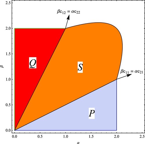
The stability regions, in the parameter space $\alpha -\beta$ bifurcation diagram, of the equilibrium points are depicted in Figure 1. In region $\mathbf{P}$ the exclusion equilibrium point on the x-axis is locally asymptotically stable having a period-doubling bifurcation at $\alpha =2$ and $\beta c_{11}<\alpha c_{21}$, with α as a bifurcation parameter. In region $\mathbf{Q}$ the exclusion equilibrium point on the y-axis is locally asymptotically stable, having a period-doubling bifurcation at $\beta =2$ and $\beta c_{12}>\alpha c_{22}$, with β as a bifurcation parameter. In region $\mathbf{S}$ the survival equilibrium point is locally asymptotically stable. On the hyperbola occurs a period-doubling bifurcation with respect to the parameters α and β.

Figure 1. Stability regions, in the $\alpha -\beta$ parameter plane, of the equilibrium points in the Ricker competition model without evolution when $c_{12}=c_{21}=0.5$ and $c_{11}=c_{22}=1$.

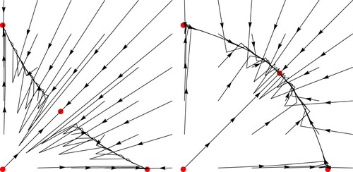
In Ref. [3], the authors proved the following result on the global dynamics of the Ricker model with no evolution

Theorem 3.1

[3]

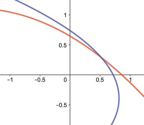
For the Ricker map with $\alpha ,\beta \in (0,2]$, the following statements hold true:

1. If $\frac{c_{12}}{c_{22}}<\frac{\alpha }{\beta }<\frac{c_{11}}{c_{21}}$, then the unique interior equilibrium point ${\mathbf{\text{E}}}^{\ast }$ is globally asymptotically stable in the interior of ${\mathbb{R}}_{+}^2$ and each of the axial equilibrium points ${\mathbf{\text{E}}}_x^{\ast }$ and ${\mathbf{\text{E}}}_y^{\ast }$ is a saddle point with the positive half-axis as its stable manifold and the heteroclinic orbit from this survival equilibrium point to ${\mathbf{\text{E}}}^{\ast }$ as its unstable manifold. (see Figure 2).

2. If $\frac{c_{12}}{c_{22}}>\frac{\alpha }{\beta }>\frac{c_{11}}{c_{21}}$, then the unique survival equilibrium point ${\mathbf{\text{E}}}^{\ast }$ is a saddle point with orbits from ${\mathbf{\text{E}}}_0^{\ast }$ to ${\mathbf{\text{E}}}^{\ast }$ as part of the stable manifold $W^s({\mathbf{\text{E}}}^{\ast })$, which divides ${\mathbb{R}}_{+}^2\setminus \{{\mathbf{\text{E}}}_0^{\ast }\}$ into two open disjoint regions $R_1,R_2$ with ${\mathbb{R}}_{+}^2\setminus \{{\mathbf{\text{E}}}_0^{\ast }\}=R_1\cup W^s({\mathbf{\text{E}}}^{\ast })\cup R_2$ where ${\mathbf{\text{E}}}_y^{\ast }\in R_1$ and ${\mathbf{\text{E}}}_x^{\ast }\in R_2$. Each of the axial equilibrium points is asymptotically stable with $R_1$ or $R_2$ as its basin of attraction.

Figure 2. Examples of dynamics catalogued in Theorem 3.1. In the left graph we use $\alpha =\beta =0.5$, $c_{12}=c_{21}=1.5$, $c_{11}=c_{22}=1$ while in the right $\alpha =\beta =1.25$, $c_{12}=c_{21}=0.5$ and $c_{11}=c_{22}=1$.

Remark 3.1

The conditions $\alpha ,\beta \in (0,2]$ and $\frac{c_{12}}{c_{22}}<\frac{\alpha }{\beta }<\frac{c_{11}}{c_{21}}$ in the hypothesis of Theorem 3.1 (a) are parts of the conditions of local stability, as it may be seen in Figure 1. Note that the vertex of the hyperbola is the point $(2,2)$ (see [17] for more details).

4. Stability of evolutionary models

We first assume that species y has no evolution, as defined by system (13(13) $\{\begin{array}{l}x(t+1)=x(t)e^{\alpha -u^2(t)/2-c_{11}(0)x(t)-c_{12}y(t)}\\ y(t+1)=y(t)e^{\beta -c_{21}x(t)-c_{22}(0)y(t)}\\ u(t+1)=(1-{\sigma }^2)u(t)-{\sigma }^2{c}_{1}x(t)\end{array}.$(13) ), i.e. $b(v_2)=\beta$ and ${\sigma }_2=0$. Then we study the model where both species evolve.

4.1. Constant trait in one species

Let $F(\mathbf{x})=(x{e}^{\alpha -u^2/2-c_{11}(0)x-c_{12}y},y{e}^{\beta -c_{21}x-c_{22}(0)y},(1-{\sigma }^2)u-{\sigma }^2{c}_{1}x)$be the map representing System (13(13) $\{\begin{array}{l}x(t+1)=x(t)e^{\alpha -u^2(t)/2-c_{11}(0)x(t)-c_{12}y(t)}\\ y(t+1)=y(t)e^{\beta -c_{21}x(t)-c_{22}(0)y(t)}\\ u(t+1)=(1-{\sigma }^2)u(t)-{\sigma }^2{c}_{1}x(t)\end{array}.$(13) ), where $\mathbf{x}=(x,y,u)$ and we replace ${\sigma }_1$ by σ for simplicity.

The Jacobian matrix of the map F is given by $\begin{array}{rl}JF(\mathbf{x})& =(\begin{array}{cc}(1-c_{11}(0)x)e^{\alpha -\frac{u^2}{2}-c_{11}(0)x-c_{12}y}& -c_{12}x{e}^{\alpha -\frac{u^2}{2}-c_{11}(0)x-c_{12}y}\\ -c_{21}y{e}^{\beta -c_{21}x-c_{22}(0)y}& (1-c_{22}(0)y)e^{\beta -c_{21}x-c_{22}(0)y}\\ -{\sigma }^2{c}_1& 0\end{array}\\ & \begin{array}{c}-xu{e}^{\alpha -\frac{u^2}{2}-c_{11}(0)x-c_{12}y}\\ 0\\ 1-{\sigma }^2\end{array}).\end{array}$We should mention that when $c_1=0$, the local dynamics of the decoupled Model (13(13) $\{\begin{array}{l}x(t+1)=x(t)e^{\alpha -u^2(t)/2-c_{11}(0)x(t)-c_{12}y(t)}\\ y(t+1)=y(t)e^{\beta -c_{21}x(t)-c_{22}(0)y(t)}\\ u(t+1)=(1-{\sigma }^2)u(t)-{\sigma }^2{c}_{1}x(t)\end{array}.$(13) ) is the same as the model without evolution (10(10) $\{\begin{array}{l}x(t+1)=ax(t)e^{-c_{11}x(t)-c_{12}y(t)}\\ y(t+1)=by(t)e^{-c_{21}x(t)-c_{22}y(t)}\end{array},$(10) ) whenever ${\sigma }^2<2$. In order to see this fact, firstly from $u(t+1)=(1-{\sigma }^2)u(t)$ we get $u(t)=(1-{\sigma }^2{)}^t{u}_0$. Hence, $u(t)\to 0$ as $t\to \mathrm{\infty }$. Secondly, at the equilibrium point $(x^{\ast },y^{\ast },0)$, the eigenvalues of $JF((x^{\ast },y^{\ast },0))$ are $\{{\lambda }_1,{\lambda }_2,1-{\sigma }^2\}$, where ${\lambda }_1$ and ${\lambda }_2$ are the same eigenvalues of the Jacobian of the two-dimensional map given by System (10(10) $\{\begin{array}{l}x(t+1)=ax(t)e^{-c_{11}x(t)-c_{12}y(t)}\\ y(t+1)=by(t)e^{-c_{21}x(t)-c_{22}y(t)}\end{array},$(10) ). Therefore, the conditions of the local stability will be the same and we have the following result.

Theorem 4.1

Let $c_1=0$, $E^{\ast }=(x^{\ast },y^{\ast },0)$ be an equilibrium point of Model (13(13) $\{\begin{array}{l}x(t+1)=x(t)e^{\alpha -u^2(t)/2-c_{11}(0)x(t)-c_{12}y(t)}\\ y(t+1)=y(t)e^{\beta -c_{21}x(t)-c_{22}(0)y(t)}\\ u(t+1)=(1-{\sigma }^2)u(t)-{\sigma }^2{c}_{1}x(t)\end{array}.$(13) ), and the speed of evolution ${\sigma }^2<2$. Then the survival equilibrium point $E^{\ast }$ is locally asymptotically stable by linearization (unstable) if $(x^{\ast },y^{\ast })$ is a locally asymptotically stable (unstable) equilibrium point of Model (10(10) $\{\begin{array}{l}x(t+1)=ax(t)e^{-c_{11}x(t)-c_{12}y(t)}\\ y(t+1)=by(t)e^{-c_{21}x(t)-c_{22}y(t)}\end{array},$(10) ) by linearization.

Remark 4.1

Obviously, if in the conditions of Theorem 4.1, we assume that ${\sigma }^2\ge 2$, any equilibrium point of Model (13(13) $\{\begin{array}{l}x(t+1)=x(t)e^{\alpha -u^2(t)/2-c_{11}(0)x(t)-c_{12}y(t)}\\ y(t+1)=y(t)e^{\beta -c_{21}x(t)-c_{22}(0)y(t)}\\ u(t+1)=(1-{\sigma }^2)u(t)-{\sigma }^2{c}_{1}x(t)\end{array}.$(13) ) is unstable.

From now on, we consider $c_1\ne 0$. Since the purpose of the model (13(13) $\{\begin{array}{l}x(t+1)=x(t)e^{\alpha -u^2(t)/2-c_{11}(0)x(t)-c_{12}y(t)}\\ y(t+1)=y(t)e^{\beta -c_{21}x(t)-c_{22}(0)y(t)}\\ u(t+1)=(1-{\sigma }^2)u(t)-{\sigma }^2{c}_{1}x(t)\end{array}.$(13) ) is applications in population dynamics, we discard equilibrium points with negative population densities (negative trait values are allowed) and obtain the following equilibrium points $E_0^{\ast }=(0,0,0),E_y^{\ast }=(0,\frac{\beta }{c_{22}(0)},0),E_{xu}^{\ast }=(\frac{A}{c_1^2},0,-{\displaystyle \frac{A}{c_1}})$and $\begin{array}{rl}{E}^{\ast }& =(\frac{c_{12}{c}_{21}-c_{11}(0)c_{22}(0)+\mathrm{\Delta }}{c_{22}(0)c_1^2},\frac{c_{11}(0)c_{22}(0)c_{21}+c_1^2{c}_{22}(0)\beta -c_{12}{c}_{21}^2-c_{21}\mathrm{\Delta }}{c_1^2{c}_{22}^2(0)},\\ & -\frac{c_{12}{c}_{21}-c_{11}(0)c_{22}(0)+\mathrm{\Delta }}{c_1{c}_{22}(0)}),\end{array}$where (15) $A=-c_{11}(0)+\sqrt{c_{11}^2(0)+2c_1^2\alpha }$(15) and (16) $\mathrm{\Delta }=\sqrt{(c_{12}{c}_{21}-c_{11}(0)c_{22}(0){)}^2+2c_1^2{c}_{22}(0)(c_{22}(0)\alpha -c_{12}\beta )}.$(16) We will refer the equilibrium point $E_0^{\ast }$ as the extinction fixed point, the equilibrium points $E_y^{\ast }$ and $E_{xu}^{\ast }$ as the exclusion equilibrium points and the equilibrium point $E^{\ast }$ as the survival equilibrium point.

At the extinction equilibrium point $E_0^{\ast }$ we have $JF(E_0^{\ast })=\left(\begin{array}{ccc}{e}^{\alpha }& 0& 0\\ 0& e^{\beta }& 0\\ -{\sigma }^2{c}_1& 0& 1-{\sigma }^2\end{array}\right).$Since $\alpha >0$ and $\beta >0$, it follows that the origin is an unstable equilibrium point if ${\sigma }^2>2$ and a saddle equilibrium point if ${\sigma }^2<2$.

Theorem 4.2

The extinction equilibrium point $E_0^{\ast }$ of the model (13(13) $\{\begin{array}{l}x(t+1)=x(t)e^{\alpha -u^2(t)/2-c_{11}(0)x(t)-c_{12}y(t)}\\ y(t+1)=y(t)e^{\beta -c_{21}x(t)-c_{22}(0)y(t)}\\ u(t+1)=(1-{\sigma }^2)u(t)-{\sigma }^2{c}_{1}x(t)\end{array}.$(13) ) is unstable. More precisely, it is source if ${\sigma }^2>2$ and a saddle equilibrium point if ${\sigma }^2<2$.

For the equilibrium point on the y-axis, we have $JF(E_y^{\ast })=\left(\begin{array}{ccc}{e}^{\alpha -\frac{c_{12}\beta }{c_{22}(0)}}& 0& 0\\ -{\displaystyle \frac{c_{21}\beta }{c_{22}(0)}}& 1-\beta & 0\\ -c_1{\sigma }^2& 0& 1-{\sigma }^2\end{array}\right).$Thus, we have the following result concerning the stability of $E_y^{\ast }$.

Theorem 4.3

The equilibrium point $E_y^{\ast }$ of model (13(13) $\{\begin{array}{l}x(t+1)=x(t)e^{\alpha -u^2(t)/2-c_{11}(0)x(t)-c_{12}y(t)}\\ y(t+1)=y(t)e^{\beta -c_{21}x(t)-c_{22}(0)y(t)}\\ u(t+1)=(1-{\sigma }^2)u(t)-{\sigma }^2{c}_{1}x(t)\end{array}.$(13) ) is:

1. locally asymptotically stable if $c_{22}(0)\alpha <c_{12}\beta$, $0<\beta <2$, and ${\sigma }^2<2$;

2. a source if $c_{22}(0)\alpha >c_{12}\beta$, $\beta >2$, and ${\sigma }^2>2$;

3. a saddle if $c_{22}(0)\alpha >c_{12}\beta$ or ${\sigma }^2>2$ with $0<\beta <2$.

We recall [14, page 248] that all the roots of a cubic polynomial ${\lambda }^3+p_1{\lambda }^2+p_2\lambda +p_3,$lie inside the unit circle if and only if (17) $|p_1+p_3|<1+p_2\text{ and }|p_2-p_1{p}_3|<1-p_3^2.$(17) If the polynomial is the characteristic polynomial of a three dimension matrix, then $p_1$ is the trace of the matrix, $p_2$ is the sum of the principal minors of the matrix and $p_3$ is the determinant of the matrix. Conditions (17(17) $|p_1+p_3|<1+p_2\text{ and }|p_2-p_1{p}_3|<1-p_3^2.$(17) ) can be applied to the Jacobian of a three-dimensional discrete dynamical system to obtain local stability results from the linearization principle (see [18]).

Since the conditions (17(17) $|p_1+p_3|<1+p_2\text{ and }|p_2-p_1{p}_3|<1-p_3^2.$(17) ) for the equilibrium points $E_{xu}^{\ast }$ and $E^{\ast }$ are long, we present only the conclusions of this analysis and in Appendix 1, we provide details. The derivation and application of the results generally require the use of some algebraic software such as Mathematica or Maple.

Theorem 4.4

Let ${\sigma }^2<2$ and $c_1\ne 0$. The equilibrium point $E_{xu}^{\ast }$ of System (13(13) $\{\begin{array}{l}x(t+1)=x(t)e^{\alpha -u^2(t)/2-c_{11}(0)x(t)-c_{12}y(t)}\\ y(t+1)=y(t)e^{\beta -c_{21}x(t)-c_{22}(0)y(t)}\\ u(t+1)=(1-{\sigma }^2)u(t)-{\sigma }^2{c}_{1}x(t)\end{array}.$(13) ) is

1. locally asymptotically stable whenever inequalities (A1(A1) $\begin{array}{rl}& c_{11}(0)A({\sigma }^2+2)<2c_1^2({\sigma }^2\alpha -{\sigma }^2+2),\end{array}$(A1) ), (A2(A2) $\begin{array}{rl}& (1-e^{\beta -\frac{A{c}_{21}}{c_1^2}})(2c_1^2\alpha -c_{11}(0)A)>0,\end{array}$(A2) ), (A3(A3) $\begin{array}{rl}& c_1^2{c}_{11}(0)A(e^{\beta -\frac{c_{21}A}{c_1^2}}+{\sigma }^2+1)-c_1^4((2\alpha -1){\sigma }^2-({\sigma }^2-2)e^{\beta -\frac{c_{21}A}{c_1^2}})>\\ & e^{\beta -\frac{c_{21}A}{c_1^2}}(c_1^2((2\alpha -1){\sigma }^2+1)-c_{11}(0)({\sigma }^2+1)A)\\ & \times (c_1^2({\sigma }^2((2\alpha -1)e^{\beta -\frac{c_{21}A}{c_1^2}}+1)-2)-c_{11}(0)A(({\sigma }^2+1)e^{\beta -\frac{c_{21}A}{c_1^2}}-1))\end{array}$(A3) ) and (A4(A4) $\begin{array}{rl}& c_1^4(2+(2\alpha -1){\sigma }^2-({\sigma }^2-2)e^{\beta -\frac{c_{21}A}{c_1^2}})-c_1^2{c}_{11}(0)A(e^{\beta -\frac{c_{21}A}{c_1^2}}+{\sigma }^2+1)>\\ & ((c_1^2((2\alpha -1){\sigma }^2+2)-c_{11}(0)A({\sigma }^2+1))e^{\beta -\frac{c_{21}A}{c_1^2}}-(c_1^2({\sigma }^2-2)+c_{11}(0)A)e^{2(\beta -\frac{c_{21}A}{c_1^2})})\\ & \times (c_1^2((2\alpha -1){\sigma }^2+1)-c_{11}(0)({\sigma }^2+1)A)\end{array}$(A4) ) in Appendix 1 are satisfied;

2. unstable if at least one of the inequalities (A1(A1) $\begin{array}{rl}& c_{11}(0)A({\sigma }^2+2)<2c_1^2({\sigma }^2\alpha -{\sigma }^2+2),\end{array}$(A1) ), (A2(A2) $\begin{array}{rl}& (1-e^{\beta -\frac{A{c}_{21}}{c_1^2}})(2c_1^2\alpha -c_{11}(0)A)>0,\end{array}$(A2) ), (A3(A3) $\begin{array}{rl}& c_1^2{c}_{11}(0)A(e^{\beta -\frac{c_{21}A}{c_1^2}}+{\sigma }^2+1)-c_1^4((2\alpha -1){\sigma }^2-({\sigma }^2-2)e^{\beta -\frac{c_{21}A}{c_1^2}})>\\ & e^{\beta -\frac{c_{21}A}{c_1^2}}(c_1^2((2\alpha -1){\sigma }^2+1)-c_{11}(0)({\sigma }^2+1)A)\\ & \times (c_1^2({\sigma }^2((2\alpha -1)e^{\beta -\frac{c_{21}A}{c_1^2}}+1)-2)-c_{11}(0)A(({\sigma }^2+1)e^{\beta -\frac{c_{21}A}{c_1^2}}-1))\end{array}$(A3) ) and (A4(A4) $\begin{array}{rl}& c_1^4(2+(2\alpha -1){\sigma }^2-({\sigma }^2-2)e^{\beta -\frac{c_{21}A}{c_1^2}})-c_1^2{c}_{11}(0)A(e^{\beta -\frac{c_{21}A}{c_1^2}}+{\sigma }^2+1)>\\ & ((c_1^2((2\alpha -1){\sigma }^2+2)-c_{11}(0)A({\sigma }^2+1))e^{\beta -\frac{c_{21}A}{c_1^2}}-(c_1^2({\sigma }^2-2)+c_{11}(0)A)e^{2(\beta -\frac{c_{21}A}{c_1^2})})\\ & \times (c_1^2((2\alpha -1){\sigma }^2+1)-c_{11}(0)({\sigma }^2+1)A)\end{array}$(A4) ) is reversed. More precisely, $E_{xu}^{\ast }$ is a source if all the inequalities are reversed and is a saddle equilibrium point if at least one of the inequalities is reversed but not all.

Concerning the equilibrium point $E^{\ast }$ we have the following:

Theorem 4.5

Let ${\sigma }^2<2$, $c_1\ne 0$ and $P_1$, $P_2$ and $P_3$ be given as in Appendix 1. Then the equilibrium point $E^{\ast }$ of System (13(13) $\{\begin{array}{l}x(t+1)=x(t)e^{\alpha -u^2(t)/2-c_{11}(0)x(t)-c_{12}y(t)}\\ y(t+1)=y(t)e^{\beta -c_{21}x(t)-c_{22}(0)y(t)}\\ u(t+1)=(1-{\sigma }^2)u(t)-{\sigma }^2{c}_{1}x(t)\end{array}.$(13) ) is

1. locally asymptotically stable whenever $|P_1+P_3|<1+P_2\text{ and }|P_2-P_1{P}_3|<1-P_3^2;$

2. unstable if at least one of the above inequalities is reversed. More precisely, $E^{\ast }$ is a source if all the inequalities are reversed and is a saddle equilibrium point if at least one of the inequalities is reversed but not all.

Remark 4.2

If in the conditions of Theorems 4.4 and 4.5, we have ${\sigma }^2\ge 2$, then the respective equilibrium points are unstable.

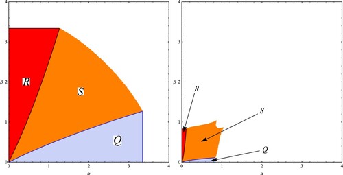
In Figure 3 we present two examples of the stability regions, in the $\alpha -\beta$ parameter plane, of the three equilibrium points $E_y^{\ast }$, $E_{xu}^{\ast }$ and $E^{\ast }$ of System (13(13) $\{\begin{array}{l}x(t+1)=x(t)e^{\alpha -u^2(t)/2-c_{11}(0)x(t)-c_{12}y(t)}\\ y(t+1)=y(t)e^{\beta -c_{21}x(t)-c_{22}(0)y(t)}\\ u(t+1)=(1-{\sigma }^2)u(t)-{\sigma }^2{c}_{1}x(t)\end{array}.$(13) ) when $c_{12}=c_{21}={\sigma }^2=0.5$, $c_{11}(0)=c_{22}(0)=1$ and $c_1=-2$. In Regions R, Q and S, the equilibrium points $E_y^{\ast }$, $E_{xu}^{\ast }$ and $E^{\ast }$ are locally asymptotically stable, respectively.

Figure 3. Two examples of the stability regions, in the $\alpha -\beta$ parameter plane, of the equilibrium points $E_y^{\ast }$, $E_{xu}^{\ast }$ and $E^{\ast }$ of the evolutionary 3-dimensional Darwinian Ricker model (13(13) $\{\begin{array}{l}x(t+1)=x(t)e^{\alpha -u^2(t)/2-c_{11}(0)x(t)-c_{12}y(t)}\\ y(t+1)=y(t)e^{\beta -c_{21}x(t)-c_{22}(0)y(t)}\\ u(t+1)=(1-{\sigma }^2)u(t)-{\sigma }^2{c}_{1}x(t)\end{array}.$(13) ). The values of the parameters are $c_{11}(0)=c_{22}(0)=1$, $c_{12}=c_{21}={\sigma }^2=0.5$ and $c_1=-2$ in the left figure and $c_1=-5$ on the right figure. The regions R, S and Q are the stability regions of the equilibrium point $E_y^{\ast }$, $E^{\ast }$ and $E_{xu}^{\ast }$, respectively. The regions will be similar in the case of positive values of $c_1$.

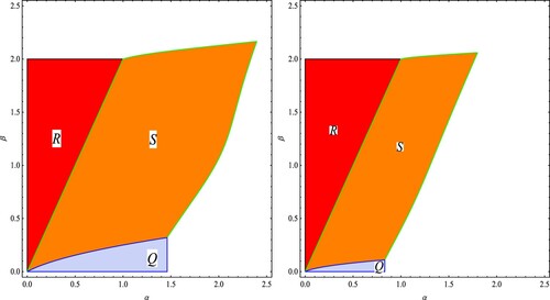
Remark 4.3

It is known that the non-evolutionary 2-species Ricker competition model (14(14) $\{\begin{array}{l}x(t+1)=x(t)e^{\alpha -c_{11}x(t)-c_{12}y(t)}\\ y(t+1)=y(t)e^{\beta -c_{21}x(t)-c_{22}y(t)}\end{array}.$(14) ) destabilizes in period-doubling bifurcation in the region $\frac{c_{12}}{c_{22}}<\frac{\alpha }{\beta }<\frac{c_{11}}{c_{21}}$ and at the boundary of the hyperbola in region S (Figure 3). For the Darwinian model of the Ricker equation (13(13) $\{\begin{array}{l}x(t+1)=x(t)e^{\alpha -u^2(t)/2-c_{11}(0)x(t)-c_{12}y(t)}\\ y(t+1)=y(t)e^{\beta -c_{21}x(t)-c_{22}(0)y(t)}\\ u(t+1)=(1-{\sigma }^2)u(t)-{\sigma }^2{c}_{1}x(t)\end{array}.$(13) ), we have the same dynamics as that of the non-evolutionary system if $c_1=0$ in the trait-dependent density coefficient $c(v-u)$. Hence, we conclude that evolution in this case has no effect on the onset of non-equilibrium and complex dynamics. In contrast, when $c_1\ne 0$, the onset of non-equilibrium and complex dynamics is accelerated to a smaller critical value of α. Moreover, the larger in absolute value the value of $c_1$, the sooner the onset of non-equilibrium and complex dynamics occurs as α is increased, as may be seen in Figure 3. It should be noted that the onset of non-equilibrium and complex dynamics can lead to either a period doubling bifurcation or to a Neimark-Sacker bifurcation. Moreover, this bifurcation may occur for values of α and β greater or smaller than 2. For instance, in Table 1, a Neimark-Sacker bifurcation occurs early for values of α slightly greater than 1.7 and β slightly greater than 0.63. And in this case evolution promotes non-equilibrium and complex dynamics. In contrast, a Neimark-Sacker bifurcation is delayed by evolution for values of α slightly greater than 2.3 and β slightly greater than 1.932, as may be seen in Table 1

Table 1. Some examples of stability of the survival equilibrium point $E^{\ast }$ of System (13(13) $\{\begin{array}{l}x(t+1)=x(t)e^{\alpha -u^2(t)/2-c_{11}(0)x(t)-c_{12}y(t)}\\ y(t+1)=y(t)e^{\beta -c_{21}x(t)-c_{22}(0)y(t)}\\ u(t+1)=(1-{\sigma }^2)u(t)-{\sigma }^2{c}_{1}x(t)\end{array}.$(13) ).

Birth Rates			Model with evolution (13(13) $\{\begin{array}{l}x(t+1)=x(t)e^{\alpha -u^2(t)/2-c_{11}(0)x(t)-c_{12}y(t)}\\ y(t+1)=y(t)e^{\beta -c_{21}x(t)-c_{22}(0)y(t)}\\ u(t+1)=(1-{\sigma }^2)u(t)-{\sigma }^2{c}_{1}x(t)\end{array}.$(13) ) – Figure 3
				Conditions
α	β	Model without evolution (Figure 1)	coefficients	$|P_1+P_3|<1+P_2$	$|P_2-P_1{P}_3|<1-P_3^2$	Real eigen- values	Stability
0.5	0.7	GS	$P_1=-1.6875$	True	True	yes	LAS
			$P_2=0.894141$
			$P_3=-0.144336$
1.2	0.7	GS	$P_1=-1.3893$	True	True	no	LAS
			$P_2=1.03411$
			$P_3=-0.230439$
2	1.05	GS	$P_1=-0.861837$	True	True	no	U
			$P_2=1.00823$
			$P_3=-0.0003149$
1.5	1.2	GS	$P_1=-0.87329$	True	True	no	LAS
			$P_2=0.528663$
			$P_3=0.122384$
2.2	2.1	U	$P_1=0.1014$	False	False	no	U
			$P_2=-0.199404$
			$P_3=0.907961$
2.3	1.932	U	$P_1=-0.0162704$	True	True	no	LAS
			$P_2=0.115483$
			$P_3=0.851567$
1.7	0.63	GS	$P_1=-1.3049$	True	True	no	LAS
			$P_2=1.33419$
			$P_3=-0.412873$

Though the sufficient conditions of stability of Theorems 4.4 and 4.5 are for the linearization principle, it may be easier to obtain sufficient conditions using Gerschgorin's Theorem [20, page 227], which estimates the location of the eigenvalues of a matrix.

Theorem 4.6

Gerschgorin's Theorem

Let $M=[m_{ij}]$ be an $n\times n$ real or complex matrix. Let ${\alpha }_i=m_{ii}$ and $r_i=\sum _{j=1,j\ne i}^n|m_{ij}|$. Then all the eigenvalues of M are inside the circles with centres ${\alpha }_i$ and radii $r_i$.

Hence to obtain sufficient conditions for asymptotic stability of an equilibrium point using Gerschgorin's theorem and the Linearization Principle, one needs to show that all the circles that contain the eigenvalues of the Jacobian matrix are located inside the unit circle in the complex plane.

Let us see the case of the equilibrium $E_{xu}^{\ast }$. For this equilibrium point we have ${\alpha }_1=(c_1^2-c_{11}(0)A)/c_1^2$, $r_1=(c_{12}|c_1|+A)A/|c_1^3|$, ${\alpha }_2=e^{\beta -c_{21}A/c_1^2}$, $r_2=0$, ${\alpha }_3=1-{\sigma }^2$ and $r_3=|c_1|{\sigma }^2$. Thus, from Gerschgorin's Theorem we have the following result concerning $E_{xu}$.

Theorem 4.7

Sufficient conditions for local stability of the equilibrium point $E_{xu}^{\ast }$ of System (13(13) $\{\begin{array}{l}x(t+1)=x(t)e^{\alpha -u^2(t)/2-c_{11}(0)x(t)-c_{12}y(t)}\\ y(t+1)=y(t)e^{\beta -c_{21}x(t)-c_{22}(0)y(t)}\\ u(t+1)=(1-{\sigma }^2)u(t)-{\sigma }^2{c}_{1}x(t)\end{array}.$(13) ) are $\begin{array}{r}A<|c_1|(c_{11}(0)-c_{12}),|c_1|(c_{11}(0)+c_{12}A)+A^2<2|c_1{|}^3,\\ c_1^2\beta <c_{21}A,|c_1|<1,{\sigma }^2(1+|c_1|)<2,\end{array}$where A is defined in (15(15) $A=-c_{11}(0)+\sqrt{c_{11}^2(0)+2c_1^2\alpha }$(15) ).

Following the same ideas, we have the following result concerning the survival equilibrium point $E^{\ast }$.

Theorem 4.8

Sufficient conditions for local stability of the survival equilibrium point $E^{\ast }$ of System (13(13) $\{\begin{array}{l}x(t+1)=x(t)e^{\alpha -u^2(t)/2-c_{11}(0)x(t)-c_{12}y(t)}\\ y(t+1)=y(t)e^{\beta -c_{21}x(t)-c_{22}(0)y(t)}\\ u(t+1)=(1-{\sigma }^2)u(t)-{\sigma }^2{c}_{1}x(t)\end{array}.$(13) ) are $\begin{array}{rl}& c_{11}(0)\mathrm{\Omega }+c_{12}+\frac{{\mathrm{\Omega }}^2}{|c_1|c_{22}(0)}<0,c_{11}(0)\mathrm{\Omega }+2>c_{12}\mathrm{\Omega }+\frac{{\mathrm{\Omega }}^2}{|c_1|c_{22}(0)}\\ & c_{22}(0)|c_1^2{c}_{22}(0)(\beta -1)-c_{21}\mathrm{\Omega }<c_1^2{c}_{22}^2(0)+c_{21}(c_{21}\mathrm{\Omega }+c_{22}(0)c_1^2\beta ),\\ & c_{22}(0)|c_1^2{c}_{22}(0)(\beta -1)-c_{21}\mathrm{\Omega }|<c_1^2{c}_{22}^2(0)-c_{21}(c_{21}\mathrm{\Omega }+c_{22}(0)c_1^2\beta ),\\ & |c_1|<1,{\sigma }^2(1+|c_1|)<2,\end{array}$where $\mathrm{\Omega }=c_{11}(0)c_{22}(0)-c_{12}{c}_{21}-\mathrm{\Delta }$, and Δ is defined in (16(16) $\mathrm{\Delta }=\sqrt{(c_{12}{c}_{21}-c_{11}(0)c_{22}(0){)}^2+2c_1^2{c}_{22}(0)(c_{22}(0)\alpha -c_{12}\beta )}.$(16) ).

4.2. Both species with evolution

Let us now consider the map $\begin{array}{rl}F(x,y,u_1,u_2)& =(x{e}^{\alpha -u_1^2/2-c_{11}(0)x-c_{12}y},y{e}^{\beta -u_2^2/2-c_{21}x-c_{22}(0)y},\\ & (1-{\sigma }_1^2)u_1-{\sigma }_1^2{c}_{1}x,(1-{\sigma }_2^2)u_2-{\sigma }_2^2{c}_{2}y)\end{array}$which represents System (12(12) $\{\begin{array}{l}x(t+1)=x(t)e^{\alpha -u_1^2(t)/2-c_{11}(0)x(t)-c_{12}y(t)}\\ y(t+1)=y(t)e^{\beta -u_2^2/2-c_{21}x(t)-c_{22}(0)y(t)}\\ u_1(t+1)=(1-{\sigma }_1^2)u_1(t)-{\sigma }_1^2{c}_{1}x(t)\\ u_2(t+1)=(1-{\sigma }_2^2)u_2(t)-{\sigma }_2^2{c}_{2}y(t)\end{array},$(12) ). Hence, the Jacobian matrix of the mapping is given by $JF(\mathbf{x})=\left(\begin{array}{cccc}(1-c_{11}(0)x)e_1& -c_{12}x{e}_1& -u_{1}x{e}_1& 0\\ -c_{21}y{e}_2& (1-c_{22}(0)y)e_2& 0& -u_{2}y{e}_2\\ -c_1{\sigma }_1^2& 0& 1-{\sigma }_1^2& 0\\ 0& -c_2{\sigma }_2^2& 0& 1-{\sigma }_2^2\end{array}\right),$where $e_1=e^{\alpha -\frac{u_1^2}{2}-c_{11}(0)x-c_{12}y}$ and $e_2=e^{\beta -\frac{u_2^2}{2}-c_{21}x-c_{22}(0)y}$.

Following arguments similar to the single species evolution model, one can see that when $c_1=c_2=0$, the dynamics of the 4D decoupled system (12(12) $\{\begin{array}{l}x(t+1)=x(t)e^{\alpha -u_1^2(t)/2-c_{11}(0)x(t)-c_{12}y(t)}\\ y(t+1)=y(t)e^{\beta -u_2^2/2-c_{21}x(t)-c_{22}(0)y(t)}\\ u_1(t+1)=(1-{\sigma }_1^2)u_1(t)-{\sigma }_1^2{c}_{1}x(t)\\ u_2(t+1)=(1-{\sigma }_2^2)u_2(t)-{\sigma }_2^2{c}_{2}y(t)\end{array},$(12) ) is the same as the 2D Ricker competition model (10(10) $\{\begin{array}{l}x(t+1)=ax(t)e^{-c_{11}x(t)-c_{12}y(t)}\\ y(t+1)=by(t)e^{-c_{21}x(t)-c_{22}y(t)}\end{array},$(10) ) without evolution if ${\sigma }_i^2<2$, i = 1, 2. Therefore, the conditions on local stability obtained by linearization will be the same as the non-evolutionary model and we have the following result.

Theorem 4.9

Let $c_i=0$, ${\sigma }_i^2<2$, i = 1, 2 and $E^{\ast }=(x^{\ast },y^{\ast },0,0)$ an equilibrium point of Model (12(12) $\{\begin{array}{l}x(t+1)=x(t)e^{\alpha -u_1^2(t)/2-c_{11}(0)x(t)-c_{12}y(t)}\\ y(t+1)=y(t)e^{\beta -u_2^2/2-c_{21}x(t)-c_{22}(0)y(t)}\\ u_1(t+1)=(1-{\sigma }_1^2)u_1(t)-{\sigma }_1^2{c}_{1}x(t)\\ u_2(t+1)=(1-{\sigma }_2^2)u_2(t)-{\sigma }_2^2{c}_{2}y(t)\end{array},$(12) ). Then $E^{\ast }$ is locally asymptotically stable by linearization (unstable) if $(x^{\ast },y^{\ast })$ is a locally asymptotically stable (unstable) equilibrium point of Model (10(10) $\{\begin{array}{l}x(t+1)=ax(t)e^{-c_{11}x(t)-c_{12}y(t)}\\ y(t+1)=by(t)e^{-c_{21}x(t)-c_{22}y(t)}\end{array},$(10) ) by linearization.

Remark 4.4

Obviously, if in the conditions of Theorem 4.9 we assume that ${\sigma }_i^2>2$, i = 1, 2, any equilibrium point of Model (12(12) $\{\begin{array}{l}x(t+1)=x(t)e^{\alpha -u_1^2(t)/2-c_{11}(0)x(t)-c_{12}y(t)}\\ y(t+1)=y(t)e^{\beta -u_2^2/2-c_{21}x(t)-c_{22}(0)y(t)}\\ u_1(t+1)=(1-{\sigma }_1^2)u_1(t)-{\sigma }_1^2{c}_{1}x(t)\\ u_2(t+1)=(1-{\sigma }_2^2)u_2(t)-{\sigma }_2^2{c}_{2}y(t)\end{array},$(12) ) is unstable.

Now, if either $c_1=0$ or $c_2=0$, then the dynamics of System (12(12) $\{\begin{array}{l}x(t+1)=x(t)e^{\alpha -u_1^2(t)/2-c_{11}(0)x(t)-c_{12}y(t)}\\ y(t+1)=y(t)e^{\beta -u_2^2/2-c_{21}x(t)-c_{22}(0)y(t)}\\ u_1(t+1)=(1-{\sigma }_1^2)u_1(t)-{\sigma }_1^2{c}_{1}x(t)\\ u_2(t+1)=(1-{\sigma }_2^2)u_2(t)-{\sigma }_2^2{c}_{2}y(t)\end{array},$(12) ) is similar to the 3D system studied in the previous section whenever either ${\sigma }_1^2<2$ or ${\sigma }_2^2<2$, respectively. Let us consider the case when $c_1\ne 0$ and $c_2=0$ (the case $c_1=0$ and $c_2\ne 0$ is similar). Hence, we have the decoupled system given by (18) $\{\begin{array}{l}x(t+1)=x(t)e^{\alpha -u_1^2(t)/2-c_{11}(0)x(t)-c_{12}y(t)}\\ y(t+1)=y(t)e^{\beta -u_2^2/2-c_{21}x(t)-c_{22}(0)y(t)}\\ u_1(t+1)=(1-{\sigma }_1^2)u_1(t)-{\sigma }_1^2{c}_{1}x(t)\\ u_2(t+1)=(1-{\sigma }_2^2)u_2(t)\end{array}.$(18) Notice that $u_2(t)\to 0$ as $t\to \mathrm{\infty }$. The Jacobian of the map given by System (12(12) $\{\begin{array}{l}x(t+1)=x(t)e^{\alpha -u_1^2(t)/2-c_{11}(0)x(t)-c_{12}y(t)}\\ y(t+1)=y(t)e^{\beta -u_2^2/2-c_{21}x(t)-c_{22}(0)y(t)}\\ u_1(t+1)=(1-{\sigma }_1^2)u_1(t)-{\sigma }_1^2{c}_{1}x(t)\\ u_2(t+1)=(1-{\sigma }_2^2)u_2(t)-{\sigma }_2^2{c}_{2}y(t)\end{array},$(12) ), evaluated at a point of the form $(x,y,u_1,0)$ has eigenvalues $\{{\lambda }_1,{\lambda }_2,{\lambda }_3,1-{\sigma }_2^2\}$, where the eigenvalues ${\lambda }_i$, i = 1, 2, 3 are the same as the eigenvalues of the Jacobian of the map given by the 3D system studied in Subsection 4.1. Therefore, the conditions of local stability obtained by the linearization principle will be the same. Hence,

Theorem 4.10

Let $c_1\ne 0$, $c_2=0$, ${\sigma }_2^2<2$ and $E^{\ast }=(x^{\ast },y^{\ast },u_1^{\ast },0)$ an equilibrium point of Model (18(18) $\{\begin{array}{l}x(t+1)=x(t)e^{\alpha -u_1^2(t)/2-c_{11}(0)x(t)-c_{12}y(t)}\\ y(t+1)=y(t)e^{\beta -u_2^2/2-c_{21}x(t)-c_{22}(0)y(t)}\\ u_1(t+1)=(1-{\sigma }_1^2)u_1(t)-{\sigma }_1^2{c}_{1}x(t)\\ u_2(t+1)=(1-{\sigma }_2^2)u_2(t)\end{array}.$(18) ). Then $E^{\ast }$ is locally asymptotically stable by linearization (unstable) if $(x^{\ast },y^{\ast },u_1^{\ast })$ is a locally asymptotically stable (unstable) equilibrium point of Model (13(13) $\{\begin{array}{l}x(t+1)=x(t)e^{\alpha -u^2(t)/2-c_{11}(0)x(t)-c_{12}y(t)}\\ y(t+1)=y(t)e^{\beta -c_{21}x(t)-c_{22}(0)y(t)}\\ u(t+1)=(1-{\sigma }^2)u(t)-{\sigma }^2{c}_{1}x(t)\end{array}.$(13) ) by linearization.

Remark 4.5

Obviously, if in the conditions of Theorem 4.10 we assume that ${\sigma }_2^2>2$, all equilibrium points of Model (18(18) $\{\begin{array}{l}x(t+1)=x(t)e^{\alpha -u_1^2(t)/2-c_{11}(0)x(t)-c_{12}y(t)}\\ y(t+1)=y(t)e^{\beta -u_2^2/2-c_{21}x(t)-c_{22}(0)y(t)}\\ u_1(t+1)=(1-{\sigma }_1^2)u_1(t)-{\sigma }_1^2{c}_{1}x(t)\\ u_2(t+1)=(1-{\sigma }_2^2)u_2(t)\end{array}.$(18) ) are unstable.

From now on, we assume that $c_i\ne 0$, i = 1, 2. The equilibrium points of the map F with non-negative densities are ${\mathbf{O}}^{\mathbf{\ast }}=(0,0,0,0)$, ${\mathbf{E}}_{\mathbf{x}{\mathbf{u}}_{\mathbf{1}}}^{\mathbf{\ast }}=({\mathrm{\Delta }}_1,0,-c_1{\mathrm{\Delta }}_1,0)$, ${\mathbf{E}}_{\mathbf{y}{\mathbf{u}}_{\mathbf{2}}}^{\mathbf{\ast }}=(0,{\mathrm{\Delta }}_2,0,-c_2{\mathrm{\Delta }}_2)$, where $c_1^2{\mathrm{\Delta }}_1=-c_{11}(0)+\sqrt{c_{11}(0{)}^2+2c_1^2\alpha }$ and $c_2^2{\mathrm{\Delta }}_2=-c_{22}(0)+\sqrt{c_{22}^2(0)+2c_2^2\beta }$, and a possible survival equilibrium point of the form ${\mathbf{E}}^{\mathbf{\ast }}=(x^{\ast },y^{\ast },-c_1{x}^{\ast },-c_2{y}^{\ast })$, $x^{\ast }>0$ and $y^{\ast }>0$. We remark here that we omit the coordinates of ${\mathbf{E}}^{\mathbf{\ast }}$ since they are big expressions and it is not practical to write them. In order to see the existence and uniqueness of the survival equilibrium point ${\mathbf{E}}^{\mathbf{\ast }}$ we observe that $x^{\ast }$ and $y^{\ast }$ are the solutions of the system $y=\frac{\alpha -0.5c_1^2{x}^2-c_{11}(0)x}{c_{12}}\text{ and }x=\frac{\beta -0.5c_2^2{y}^2-c_{22}(0)y}{c_{21}}.$In the first quadrant of the x−y plane, these two parabolas are concave and monotone. Hence, they intersect in at most one point, and consequently, we have either one or no positive interior equilibrium point as shown in Figures 4 and 5.

Figure 4. The two isoclines do not intersect in the interior of ${\mathbb{R}}^2$, and thus we have no positive interior equilibrium points in System (12(12) $\{\begin{array}{l}x(t+1)=x(t)e^{\alpha -u_1^2(t)/2-c_{11}(0)x(t)-c_{12}y(t)}\\ y(t+1)=y(t)e^{\beta -u_2^2/2-c_{21}x(t)-c_{22}(0)y(t)}\\ u_1(t+1)=(1-{\sigma }_1^2)u_1(t)-{\sigma }_1^2{c}_{1}x(t)\\ u_2(t+1)=(1-{\sigma }_2^2)u_2(t)-{\sigma }_2^2{c}_{2}y(t)\end{array},$(12) ). Here we use $\alpha =\ln (3)$, $\beta =\ln (4.2)$, $c_1=0.8$, $c_2=-1.6$, $c_{11}(0)=c_{22}(0)=1$, $c_{12}=1.3$ and $c_{21}=2.8$.

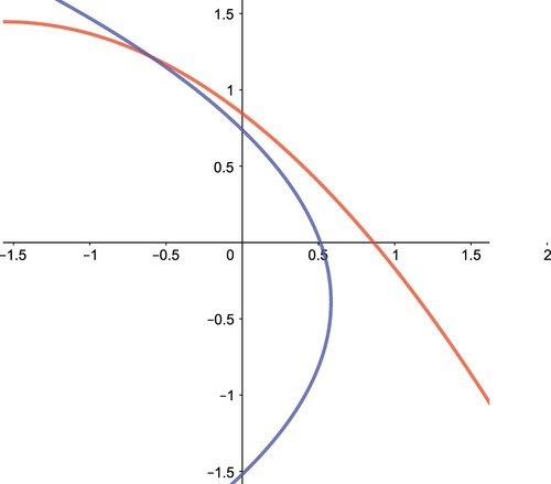
Figure 5. The two isoclines intersect at one point in the interior of ${\mathbb{R}}^2$, and thus we have one interior equilibrium point in System (12(12) $\{\begin{array}{l}x(t+1)=x(t)e^{\alpha -u_1^2(t)/2-c_{11}(0)x(t)-c_{12}y(t)}\\ y(t+1)=y(t)e^{\beta -u_2^2/2-c_{21}x(t)-c_{22}(0)y(t)}\\ u_1(t+1)=(1-{\sigma }_1^2)u_1(t)-{\sigma }_1^2{c}_{1}x(t)\\ u_2(t+1)=(1-{\sigma }_2^2)u_2(t)-{\sigma }_2^2{c}_{2}y(t)\end{array},$(12) ). Here we use $\alpha =\ln (3)$, $\beta =\ln (4.2)$, $c_1=0.8$, $c_2=-1.6$, $c_{11}(0)=c_{22}(0)=1$, $c_{12}=1.8$ and $c_{21}=2.1$.

At the origin we have $JF({\mathbf{O}}^{\ast })=\left(\begin{array}{cccc}{e}^{\alpha }& 0& 0& 0\\ 0& e^{\beta }& 0& 0\\ -c_1{\sigma }_1^2& 0& 1-{\sigma }_1^2& 0\\ 0& -c_2{\sigma }_2^2& 0& 1-{\sigma }_2^2\end{array}\right).$Hence, the origin is an unstable equilibrium point provide that $\alpha ,\beta >0$.

Theorem 4.11

The origin is an unstable equilibrium point of the model (12(12) $\{\begin{array}{l}x(t+1)=x(t)e^{\alpha -u_1^2(t)/2-c_{11}(0)x(t)-c_{12}y(t)}\\ y(t+1)=y(t)e^{\beta -u_2^2/2-c_{21}x(t)-c_{22}(0)y(t)}\\ u_1(t+1)=(1-{\sigma }_1^2)u_1(t)-{\sigma }_1^2{c}_{1}x(t)\\ u_2(t+1)=(1-{\sigma }_2^2)u_2(t)-{\sigma }_2^2{c}_{2}y(t)\end{array},$(12) ) provide that $\alpha >0$ and $\beta >0$. More precisely, it is a source if ${\sigma }_i^2>2$, i = 1, 2 and a saddle if ${\sigma }_1^2<2$ or ${\sigma }_2^2<2$.

Let us recall that for a polynomial of the form ${\lambda }^4+p_1{\lambda }^3+p_2{\lambda }^2+p_3\lambda +p_4,$all the roots lie inside the unit circle [16] whenever (19) $\begin{array}{rl}\text{Necessary Conditions: }& |p_1+p_3|<1+p_2+p_4,\\ \text{Sufficient Conditions: }& |p_4|<1,|p_1{p}_4-p_3|<1-p_4^2\\ & |(p_4^2-1{)}^2-(p_4{p}_1-p_3{)}^2|\\ & >|(p_4^2-1)p_2(p_4-1)-(p_3{p}_4-p_1)(p_1{p}_4-p_3)|.\end{array}$(19) In Appendix 2, we determine the coefficients of the characteristic polynomial of the Jacobin matrix evaluated in each one of the equilibrium points ${\mathbf{E}}_{\mathbf{x}{\mathbf{u}}_{\mathbf{1}}}^{\mathbf{\ast }}$, ${\mathbf{E}}_{\mathbf{y}{\mathbf{u}}_{\mathbf{2}}}^{\mathbf{\ast }}$ and ${\mathbf{E}}^{\mathbf{\ast }}$ of System (12(12) $\{\begin{array}{l}x(t+1)=x(t)e^{\alpha -u_1^2(t)/2-c_{11}(0)x(t)-c_{12}y(t)}\\ y(t+1)=y(t)e^{\beta -u_2^2/2-c_{21}x(t)-c_{22}(0)y(t)}\\ u_1(t+1)=(1-{\sigma }_1^2)u_1(t)-{\sigma }_1^2{c}_{1}x(t)\\ u_2(t+1)=(1-{\sigma }_2^2)u_2(t)-{\sigma }_2^2{c}_{2}y(t)\end{array},$(12) ). This leads to the following results:

Theorem 4.12

Let $c_i\ne 0$ and ${\sigma }_i^2<2$, i = 1, 2. The equilibrium point ${\mathbf{E}}_{\mathbf{y}{\mathbf{u}}_{\mathbf{2}}}^{\mathbf{\ast }}$ (respectively ${\mathbf{E}}_{\mathbf{x}{\mathbf{u}}_{\mathbf{1}}}^{\mathbf{\ast }}$) of System (12(12) $\{\begin{array}{l}x(t+1)=x(t)e^{\alpha -u_1^2(t)/2-c_{11}(0)x(t)-c_{12}y(t)}\\ y(t+1)=y(t)e^{\beta -u_2^2/2-c_{21}x(t)-c_{22}(0)y(t)}\\ u_1(t+1)=(1-{\sigma }_1^2)u_1(t)-{\sigma }_1^2{c}_{1}x(t)\\ u_2(t+1)=(1-{\sigma }_2^2)u_2(t)-{\sigma }_2^2{c}_{2}y(t)\end{array},$(12) ) is locally asymptotically stable whenever Conditions (19(19) $\begin{array}{rl}\text{Necessary Conditions: }& |p_1+p_3|<1+p_2+p_4,\\ \text{Sufficient Conditions: }& |p_4|<1,|p_1{p}_4-p_3|<1-p_4^2\\ & |(p_4^2-1{)}^2-(p_4{p}_1-p_3{)}^2|\\ & >|(p_4^2-1)p_2(p_4-1)-(p_3{p}_4-p_1)(p_1{p}_4-p_3)|.\end{array}$(19) ) are satisfied, where the sequence of coefficients $p_i$, i = 1, 2, 3, 4 are determined in Appendix 2.

Theorem 4.13

Let $c_i\ne 0$ and ${\sigma }_i^2<2$, i = 1, 2. The survival equilibrium point ${\mathbf{E}}^{\mathbf{\ast }}$ of System (12(12) $\{\begin{array}{l}x(t+1)=x(t)e^{\alpha -u_1^2(t)/2-c_{11}(0)x(t)-c_{12}y(t)}\\ y(t+1)=y(t)e^{\beta -u_2^2/2-c_{21}x(t)-c_{22}(0)y(t)}\\ u_1(t+1)=(1-{\sigma }_1^2)u_1(t)-{\sigma }_1^2{c}_{1}x(t)\\ u_2(t+1)=(1-{\sigma }_2^2)u_2(t)-{\sigma }_2^2{c}_{2}y(t)\end{array},$(12) ) is locally asymptotically stable whenever Conditions (19(19) $\begin{array}{rl}\text{Necessary Conditions: }& |p_1+p_3|<1+p_2+p_4,\\ \text{Sufficient Conditions: }& |p_4|<1,|p_1{p}_4-p_3|<1-p_4^2\\ & |(p_4^2-1{)}^2-(p_4{p}_1-p_3{)}^2|\\ & >|(p_4^2-1)p_2(p_4-1)-(p_3{p}_4-p_1)(p_1{p}_4-p_3)|.\end{array}$(19) ) are satisfied where the sequence of coefficients $p_i$, i = 1, 2, 3, 4 of the respective characteristic polynomial are determined in Appendix 2.

Remark 4.6

If at least one of the inequalities given by (19(19) $\begin{array}{rl}\text{Necessary Conditions: }& |p_1+p_3|<1+p_2+p_4,\\ \text{Sufficient Conditions: }& |p_4|<1,|p_1{p}_4-p_3|<1-p_4^2\\ & |(p_4^2-1{)}^2-(p_4{p}_1-p_3{)}^2|\\ & >|(p_4^2-1)p_2(p_4-1)-(p_3{p}_4-p_1)(p_1{p}_4-p_3)|.\end{array}$(19) ) is reversed in Theorem 4.12 or either ${\sigma }_1^2>2$ or ${\sigma }_2^2>2$, then the respective equilibrium point is unstable. Similarly in Theorem 4.13.

Observe that in Figure 6 the stability regions, in the parameter space bifurcation diagram $\alpha -\beta$, of the equilibrium points ${\mathbf{E}}_{\mathbf{x}{\mathbf{u}}_{\mathbf{1}}}^{\mathbf{\ast }}$, ${\mathbf{E}}_{\mathbf{y}{\mathbf{u}}_{\mathbf{2}}}^{\mathbf{\ast }}$ and ${\mathbf{E}}^{\mathbf{\ast }}$, for certain values of the parameters in two distinct cases. In Region Q, the equilibrium point ${\mathbf{E}}_{\mathbf{x}{\mathbf{u}}_{\mathbf{1}}}^{\mathbf{\ast }}$ is locally asymptotically stable, in Region R the equilibrium point ${\mathbf{E}}_{\mathbf{y}{\mathbf{u}}_{\mathbf{2}}}^{\mathbf{\ast }}$ is locally asymptotically stable while in Region S the survival equilibrium point is locally asymptotically stable. It should be noted that the onset of non-equilibrium and complex dynamics can lead to either period-doubling bifurcation or to a Neimark-Sacker bifurcation. On the left figure in Figure 6, with smaller values $c_1$ and $c_2$, the onset of complex dynamics is delayed for larger values of α and β. However, on the right figure, with larger values $c_1$ and $c_2$, the onset of complex dynamics occurs for much smaller values of α and β.

Figure 6. Stability regions, of the equilibrium points ${\mathbf{E}}_{\mathbf{x}{\mathbf{u}}_{\mathbf{1}}}^{\mathbf{\ast }}$, ${\mathbf{E}}_{\mathbf{y}{\mathbf{u}}_{\mathbf{2}}}^{\mathbf{\ast }}$ and ${\mathbf{E}}^{\mathbf{\ast }}$ of Model (12(12) $\{\begin{array}{l}x(t+1)=x(t)e^{\alpha -u_1^2(t)/2-c_{11}(0)x(t)-c_{12}y(t)}\\ y(t+1)=y(t)e^{\beta -u_2^2/2-c_{21}x(t)-c_{22}(0)y(t)}\\ u_1(t+1)=(1-{\sigma }_1^2)u_1(t)-{\sigma }_1^2{c}_{1}x(t)\\ u_2(t+1)=(1-{\sigma }_2^2)u_2(t)-{\sigma }_2^2{c}_{2}y(t)\end{array},$(12) ), in $\alpha -\beta$ parameter plane, when $c_{12}=c_{21}=0.5$, $c_{11}(0)=c_{22}(0)=1$, ${\sigma }_1={\sigma }_2=\sqrt{0.5}$ and $c_1=c_2=-0.5$ in the left figure and $c_1=c_2=-5$ in the right figure. The scenario for $c_i>0$ will originate similar figures.

5. Global stability

In this section, we will use two results that enable us to prove a general theorem on the global stability of the interior equilibrium point of our model. We first utilize a theorem on nonautonomous systems that are asymptotic to either autonomous systems or to periodic systems. This result is applied to the special case when $c_1=0$ and $c_2=0$, where the equations of the traits $u_1$ and $u_2$ decouple from the size (density) of species x and y, respectively. The final step in our analysis is to use a perturbation theorem in Ref. [27] to extend the result to our model.

5.1. Asymptotically autonomous

Let ${\mathbb{R}}_{+}^n$ denote the cone of nonnegative vectors in ${\mathbb{R}}^n$ and let $int({\mathbb{R}}_{+}^n)$ and $\mathrm{\partial }({\mathbb{R}}_{+}^n)$ denote the interior and the boundary of ${\mathbb{R}}_{+}^n$, respectively. Let $F,F_t:{\mathbb{R}}_{+}^n⟶{\mathbb{R}}_{+}^n$ to be continuous functions for all $t\in {\mathbb{Z}}_{+}$. Assume that

${\mathit{A}}_{\mathbf{1}}\mathbf{:}$ $F_t$ converges uniformly to F as $t\to \mathrm{\infty }$.

Then $\mathbf{x}\mathbf{(}\mathbf{0}\mathbf{)}\in {\mathbb{R}}_{+}^n$ implies that the solutions of the nonautonomous difference equation (20) $\mathbf{x}(t+1)=F_t(\mathbf{x}(t)),$(20) satisfies $\mathbf{x}\mathbf{(}\mathbf{t}\mathbf{)}\in {\mathbb{R}}_{+}^n$, for all $t\in {\mathbb{Z}}_{+}$ where $\mathbf{x}=(x_1,x_2,\dots ,x_n)\in {\mathbb{R}}_{+}^n$.

The same is true for solutions of the limiting equation (21) $\mathbf{x}(t+1)=F(\mathbf{x}(t)),$(21) where we assume

${\mathit{A}}_{\mathbf{2}}:$ $f_t:int({\mathbb{R}}_{+}^n)⟶int({\mathbb{R}}_{+}^n)$.

Here, it is always true that $\mathbf{x}\mathbf{(}\mathbf{0}\mathbf{)}\in int({\mathbb{R}}_{+}^n)$ implies that the solutions of the nonautonomous difference Equation (20(20) $\mathbf{x}(t+1)=F_t(\mathbf{x}(t)),$(20) ) satisfies $\mathbf{x}\mathbf{(}\mathbf{t}\mathbf{)}\in int({\mathbb{R}}_{+}^n)$, for all $t\in {\mathbb{Z}}_{+}$.

Theorem 5.1

[11, 19]

Assume ${\mathit{A}}_{\mathbf{1}}$ and ${\mathit{A}}_{\mathbf{2}}$ and the limiting equation has an equilibrium point ${\mathbf{x}}^{\ast }\in {\mathbb{R}}_{+}^n$. Then

1. if ${\mathbf{x}}^{\ast }\in int({\mathbb{R}}_{+}^n)$, and if it is globally asymptotically stable on $int({\mathbb{R}}_{+}^n)$ as an equilibrium point of limiting equation, then all solutions of the nonautonomous difference equation with $\mathbf{x}\mathbf{(}\mathbf{0}\mathbf{)}\in int({\mathbb{R}}_{+}^n)$ tend to ${\mathbf{x}}^{\ast }$.

2. if ${\mathbf{x}}^{\ast }\in \mathrm{\partial }({\mathbb{R}}_{+}^n)$, and if it is globally asymptotically stable on $int({\mathbb{R}}_{+}^n)$, then all solutions of the nonautonomous difference equation with $\mathbf{x}\mathbf{(}\mathbf{0}\mathbf{)}\in int({\mathbf{R}}_{+}^n)$ tend to ${\mathbf{x}}^{\ast }$.

5.2. A perturbation result

Consider the difference equation (22) $\mathbf{x}(t+1)=F(\mathbf{x}(t),\eta ),$(22) where $F:U\times G\to U$ is continuous, $U\subset {\mathbb{R}}_{+}^n$, $G\subset \mathbb{R}$ and $JF(\mathbf{x},\eta )$ (the Jacobian matrix) is continuous on ${\mathbb{R}}_{+}^n\times G$. The following result is adapted from Ref. [27]. Before we present the result we list one more assumption:

H: there is a compact set $M\subset U$ such that for $\eta \in G$ and $\mathbf{z}\in U$, $F^s(\mathbf{x})\in M$ for all large s, where $F^s(\mathbf{x})=F\circ F^{s-1}(\mathbf{x})$.

Theorem 5.2

Assume that $({\mathbf{x}}_0,{\eta }_0)\in U\times G$, $F({\mathbf{x}}_0,{\eta }_0)={\mathbf{x}}_0$, $\rho (JF({\mathbf{x}}_0,{\eta }_0))<1$ and ${\mathbf{x}}_0$ is globally attracting equilibrium point of (22(22) $\mathbf{x}(t+1)=F(\mathbf{x}(t),\eta ),$(22) ) when $\eta ={\eta }_0$. If in addition, we assume that H holds, then there exits $\delta >0$ and a unique ${\mathbf{x}}^{\ast }(\eta )\in U$ for $\eta \in \mathbf{B}\mathbf{(}{\eta }_{\mathbf{0}}\mathbf{,}\delta \mathbf{)}$ such that $F({\mathbf{x}}^{\ast }(\eta ),\eta )=\hat{\mathbf{x}}(\eta )$ and $F^t(\mathbf{z})\to {\mathbf{x}}^{\ast }(\eta )$ as $t\to \mathrm{\infty }$ for all $\mathbf{z}\in U$.

Now, setting $c_1=0$ and $c_2=0$ in System (12(12) $\{\begin{array}{l}x(t+1)=x(t)e^{\alpha -u_1^2(t)/2-c_{11}(0)x(t)-c_{12}y(t)}\\ y(t+1)=y(t)e^{\beta -u_2^2/2-c_{21}x(t)-c_{22}(0)y(t)}\\ u_1(t+1)=(1-{\sigma }_1^2)u_1(t)-{\sigma }_1^2{c}_{1}x(t)\\ u_2(t+1)=(1-{\sigma }_2^2)u_2(t)-{\sigma }_2^2{c}_{2}y(t)\end{array},$(12) ), yields the following system in our model (23) $\{\begin{array}{l}x(t+1)=x(t)e^{\alpha -u_1^2(t)/2-c_{11}(0)x(t)-c_{12}y(t)}\\ y(t+1)=y(t)e^{\beta -u_2^2(t)/2-c_{21}x(t)-c_{22}(0)y(t)}\\ u_1(t+1)=(1-{\sigma }_1^2)u_1(t)\\ u_2(t+1)=(1-{\sigma }_2^2)u_2(t)\end{array}.$(23) Since ${\sigma }_i^2<2$, we have $\underset{t\to \mathrm{\infty }}{lim}{u}_i(t)=0$, where the equilibrium points of $u_i(t)$ are $u_i^{\ast }=0$, i = 1, 2. The limiting system will be the classical Ricker competition model with no evolution (24) $\{\begin{array}{l}x(t+1)=x(t)e^{\alpha -c_{11}(0)x(t)-c_{12}y(t)}\\ y(t+1)=y(t)e^{\beta -c_{21}x(t)-c_{22}(0)y(t)}\end{array}.$(24) Using Theorem (3.1) and Theorem (5.2) we obtain the following global asymptotic stability result.

Theorem 5.3

Suppose all the assumptions in Theorem (3.1) hold true. Then there exists $\delta >0$ such that for each $c_i\in (-\delta ,\delta )$, $\delta <min\{|4(1-{\sigma }_1^2)/{\sigma }_1^2|,|4(1-{\sigma }_2^2)/{\sigma }_2^2|\}$, the interior equilibrium point $E_{c_1,c_2}^{\ast }=(x_{c_1}^{\ast },y_{c_2}^{\ast },u_{1c_1}^{\ast },u_{2c_2}^{\ast })$ of System (12(12) $\{\begin{array}{l}x(t+1)=x(t)e^{\alpha -u_1^2(t)/2-c_{11}(0)x(t)-c_{12}y(t)}\\ y(t+1)=y(t)e^{\beta -u_2^2/2-c_{21}x(t)-c_{22}(0)y(t)}\\ u_1(t+1)=(1-{\sigma }_1^2)u_1(t)-{\sigma }_1^2{c}_{1}x(t)\\ u_2(t+1)=(1-{\sigma }_2^2)u_2(t)-{\sigma }_2^2{c}_{2}y(t)\end{array},$(12) ) is globally asymptotically stable.

6. Conclusion

In Darwin's theory on the mechanism of evolution, competition among living species has been viewed as a major part of the ‘struggle for existence’ and therefore as a basis for natural selection (Darwin 1872 [13], Christiansen and Loeschcke 1990 [7]). Motivated by the fact that competition for limiting resources is among the most fundamental ecological interactions and has long been considered a key driver of species coexistence and biodiversity, we investigated the evolutionary dynamics of two competing species. We made the restrictive assumption that intraspecific competition is affected by the evolution of the traits of the species, while interspecific competition is not.

Our local and global analysis provides interesting and important results in both mathematics and biological insights. In Section 4, we provide theoretical results on the sufficient conditions for local stability of the interior equilibrium when one or two of the species are subject to intra-specific evolutionary adaptation. The analysis, combined with parameter space stability diagrams (e.g. see Figure 6), suggests that evolution may destablize the coexistence equilibrium of the two competing species or promote their stability depending on the speed of evolution ${\sigma }_i^2,i=1,2$. Figure 6 suggests that the faster evolutionary speed the more likely the coexistence equilibrium is stabilized. This result is in line with the work by Cushing [9]. In Cushing's paper, it was found that the speed of evolution and the degree of the intraspecific competition coefficient dependence on the evolving trait of the species play an important role in stability. For our competition model, when evolution proceeds at a faster pace, evolution promotes complex dynamics in the way that destabilization can occur when the intra-specific competition coefficient is highly sensitive to changes in the trait.

In Section 5, using Theorem 3.1 and Theorem 5.2, we provide global stability results of the 4-dimensional 2-species Ricker competition model with trait dynamics in each species. As far as we know, this is the first result in the literature on the global stability of a 4-dimensional system that is not monotone. For global stability results of 2-dimensional systems, one may refer to the paper by Smith [26] and for higher dimensional systems, one may refer to the work of Balreira, Elaydi and Luís [5]. In the paper by Ackleh et al. [1], the authors investigated the global stability of a Leslie-Gower competition model of two-species in which only one of the species is subject to evolutionary adaptations. The paper by Rael et al. [21] also deals with the evolutionary dynamics of a Leslie-Gower competition model of two-species but most of the study was based on extensive numerical simulations of the evolutionary model. It should be noted that the Leslie-Gower model is monotone and hence one can apply Smith's theory [25, 26], or the results in Balreira, Elaydi and Luís [5] to show global stability. Ackleh et al. [2] studied the dynamics of a predator-prey model with a single evolutionary trait for both the predator and the prey. This paper uses a similar perturbation approach as used here to obtain global asymptotically stability of the interior equilibrium for an evolutionary predator-prey model.

In future work, we intend to study the effects of evolution of inter-specific competition on the dynamics of our evolutionary models in order to understand the evolutionary adaptation of competing species. We also intend to study the nonautonomous evolutionary periodic Ricker competition model. By varying the competition parameters, which may be caused by fluctuating habitats, we will study the effect of the traits on the evolution of species.

Disclosure statement

No potential conflict of interest was reported by the authors.

Additional information

Funding

The research of Y.K. is partially supported by NSF-DMS (Award Number 1716802&2052820); NSF-IOS/DMS (Award Number 1558127) and The James S. McDonnell Foundation 21st Century Science Initiative in Studying Complex Systems Scholar Award (UHC Scholar Award 220020472) and the research of R.L. is partially supported by FCT/Portugal through the project UIDB/04459/2020.

Appendices

Appendix 1: Local stability conditions of the model with constant trait in one species

The Jacobian matrix evaluated at the equilibrium point $E_{xu}^{\ast }$ of Model (13(13) $\{\begin{array}{l}x(t+1)=x(t)e^{\alpha -u^2(t)/2-c_{11}(0)x(t)-c_{12}y(t)}\\ y(t+1)=y(t)e^{\beta -c_{21}x(t)-c_{22}(0)y(t)}\\ u(t+1)=(1-{\sigma }^2)u(t)-{\sigma }^2{c}_{1}x(t)\end{array}.$(13) ) is $JF(E_{xu}^{\ast })=\left(\begin{array}{ccc}{\displaystyle \frac{c_1^2-c_{11}(0)A}{c_1^2}}& -{\displaystyle \frac{c_{12}A}{c_1^2}}& {\displaystyle \frac{A^2}{c_1^3}}\\ 0& e^{\beta -{\displaystyle \frac{A{c}_{21}}{c_1^2}}}& 0\\ -{\sigma }^2{c}_1& 0& 1-{\sigma }^2\end{array}\right),$where A is in (15(15) $A=-c_{11}(0)+\sqrt{c_{11}^2(0)+2c_1^2\alpha }$(15) ). The coefficients of the characteristic polynomial of $JF(E_{xu}^{\ast })$ are $\begin{array}{rl}{p}_1& ={\sigma }^2-2+\frac{c_{11}(0)A}{c_1^2}-e^{\beta -\frac{c_{21}A}{c_1^2}},\\ p_2& =(2-{\sigma }^2-\frac{c_{11}(0)A}{c_1^2})e^{\beta -\frac{c_{21}A}{c_1^2}}+1-{\sigma }^2-\frac{(1+{\sigma }^2)c_{11}(0)A}{c_1^2}+2{\sigma }^2\alpha \\ p_3& =\frac{c_1^2({\sigma }^2-1-2{\sigma }^2\alpha )+({\sigma }^2+1)c_{11}(0)A}{c_1^2}{e}^{\beta -\frac{c_{21}A}{c_1^2}}\end{array}$Hence, we have local stability of the equilibrium point $E_{xu}^{\ast }$ whenever the following four inequalities are satisfied (A1) $\begin{array}{rl}& c_{11}(0)A({\sigma }^2+2)<2c_1^2({\sigma }^2\alpha -{\sigma }^2+2),\end{array}$(A1) (A2) $\begin{array}{rl}& (1-e^{\beta -\frac{A{c}_{21}}{c_1^2}})(2c_1^2\alpha -c_{11}(0)A)>0,\end{array}$(A2) (A3) $\begin{array}{rl}& c_1^2{c}_{11}(0)A(e^{\beta -\frac{c_{21}A}{c_1^2}}+{\sigma }^2+1)-c_1^4((2\alpha -1){\sigma }^2-({\sigma }^2-2)e^{\beta -\frac{c_{21}A}{c_1^2}})>\\ & e^{\beta -\frac{c_{21}A}{c_1^2}}(c_1^2((2\alpha -1){\sigma }^2+1)-c_{11}(0)({\sigma }^2+1)A)\\ & \times (c_1^2({\sigma }^2((2\alpha -1)e^{\beta -\frac{c_{21}A}{c_1^2}}+1)-2)-c_{11}(0)A(({\sigma }^2+1)e^{\beta -\frac{c_{21}A}{c_1^2}}-1))\end{array}$(A3) and (A4) $\begin{array}{rl}& c_1^4(2+(2\alpha -1){\sigma }^2-({\sigma }^2-2)e^{\beta -\frac{c_{21}A}{c_1^2}})-c_1^2{c}_{11}(0)A(e^{\beta -\frac{c_{21}A}{c_1^2}}+{\sigma }^2+1)>\\ & ((c_1^2((2\alpha -1){\sigma }^2+2)-c_{11}(0)A({\sigma }^2+1))e^{\beta -\frac{c_{21}A}{c_1^2}}-(c_1^2({\sigma }^2-2)+c_{11}(0)A)e^{2(\beta -\frac{c_{21}A}{c_1^2})})\\ & \times (c_1^2((2\alpha -1){\sigma }^2+1)-c_{11}(0)({\sigma }^2+1)A)\end{array}$(A4) The Jacobian matrix evaluated at the survival equilibrium point $E^{\ast }$ of Model (13(13) $\{\begin{array}{l}x(t+1)=x(t)e^{\alpha -u^2(t)/2-c_{11}(0)x(t)-c_{12}y(t)}\\ y(t+1)=y(t)e^{\beta -c_{21}x(t)-c_{22}(0)y(t)}\\ u(t+1)=(1-{\sigma }^2)u(t)-{\sigma }^2{c}_{1}x(t)\end{array}.$(13) ) is given by $JF(E^{\ast })=\left(\begin{array}{ccc}1-x^{\ast }& -c_{12}{x}^{\ast }& -u^{\ast }{x}^{\ast }\\ -c_{21}{y}^{\ast }& 1-y^{\ast }& 0\\ -{\sigma }^2{c}_1& 0& 1-{\sigma }^2\end{array}\right),$where $x^{\ast }=\frac{c_{12}{c}_{21}-c_{11}(0)c_{22}(0)+\mathrm{\Delta }}{c_{22}(0)c_1^2}$, $y^{\ast }\frac{c_{11}(0)c_{22}(0)c_{21}+c_1^2{c}_{22}(0)\beta -c_{12}{c}_{21}^2-c_{21}\mathrm{\Delta }}{c_1^2{c}_{22}^2(0)}$, $u^{\ast }=-\frac{c_{12}{c}_{21}-c_{11}(0)c_{22}(0)+\mathrm{\Delta }}{c_1{c}_{22}(0)}$ and Δ is in (16(16) $\mathrm{\Delta }=\sqrt{(c_{12}{c}_{21}-c_{11}(0)c_{22}(0){)}^2+2c_1^2{c}_{22}(0)(c_{22}(0)\alpha -c_{12}\beta )}.$(16) ).

The coefficients of the characteristic polynomial are $\begin{array}{rl}{P}_1& ={\sigma }^2+x^{\ast }+y^{\ast }-3,\\ P_2& =3-2{\sigma }^2+({\sigma }^2-2)(x^{\ast }+y^{\ast })-c_1{\sigma }^2{u}^{\ast }{x}^{\ast }+(1-c_{12}{c}_{21})x^{\ast }{y}^{\ast }\end{array}$and $P_3=c_1{\sigma }^2-u^{\ast }{x}^{\ast }(1-y^{\ast })+({\sigma }^2-1)(1-x^{\ast }-y^{\ast }+(1-c_{12}{c}_{21})x^{\ast }{y}^{\ast }).$Now, using a computer Algebra system, one may determine the inequalities $|P_1+P_3|<1+P_2$ and $|P_2-P_1{P}_3|<1-P_3^2$ and we have the sufficient conditions for local stability of $E^{\ast }$.

Appendix 2: Local stability conditions for both species with evolution

For the equilibrium point ${\mathbf{E}}_{\mathbf{y}{\mathbf{u}}_{\mathbf{2}}}^{\mathbf{\ast }}$ of Model (12(12) $\{\begin{array}{l}x(t+1)=x(t)e^{\alpha -u_1^2(t)/2-c_{11}(0)x(t)-c_{12}y(t)}\\ y(t+1)=y(t)e^{\beta -u_2^2/2-c_{21}x(t)-c_{22}(0)y(t)}\\ u_1(t+1)=(1-{\sigma }_1^2)u_1(t)-{\sigma }_1^2{c}_{1}x(t)\\ u_2(t+1)=(1-{\sigma }_2^2)u_2(t)-{\sigma }_2^2{c}_{2}y(t)\end{array},$(12) ) we have $JF({\mathbf{E}}_{\mathbf{y}{\mathbf{u}}_{\mathbf{2}}}^{\mathbf{\ast }})=\left(\begin{array}{cccc}{e}^{\alpha -c_{12}{\mathrm{\Delta }}_2}& 0& 0& 0\\ -c_{21}\mathrm{\Omega }{\mathrm{\Delta }}_2& (1-{\mathrm{\Delta }}_2)\mathrm{\Omega }& 0& c_2\mathrm{\Omega }{\mathrm{\Delta }}_2^2\\ -c_1{\sigma }_1^2& 0& 1-{\sigma }_1^2& 0\\ 0& -c_2{\sigma }_2^2& 0& 1-{\sigma }_2^2\end{array}\right),$where $\mathrm{\Omega }=e^{\frac{(c_{22}(0)-1)c_{22}(0)}{2c_2^2}}$ and ${\mathrm{\Delta }}_2$ is defined in Subsection (4.2).

Computing the coefficients of the characteristic polynomial we have $\begin{array}{rl}{p}_1& ={\sigma }_1^2+{\sigma }_2^2-2-(1-{\mathrm{\Delta }}_2)\mathrm{\Omega }-e^{\alpha -c_{12}{\mathrm{\Delta }}_2},\\ p_2& ={\sigma }_1^2(-(e^{\alpha +c_{12}{\mathrm{\Delta }}_2}-{\mathrm{\Delta }}_2\mathrm{\Omega }-{\sigma }_2^2+\mathrm{\Omega }+1))+(-{\mathrm{\Delta }}_2\mathrm{\Omega }+\mathrm{\Omega }+2)e^{\alpha +c_{12}{\mathrm{\Delta }}_2}\\ & -{\sigma }_2^2(e^{\alpha +c_{12}{\mathrm{\Delta }}_2}+\mathrm{\Omega }(-(c_2^2{\mathrm{\Delta }}_2^2+{\mathrm{\Delta }}_2-1))+1)-2{\mathrm{\Delta }}_2\mathrm{\Omega }+2\mathrm{\Omega }+1\\ p_3& =e^{\alpha +c_{12}{\mathrm{\Delta }}_2}({\sigma }_2^2(1-\mathrm{\Omega }(c_2^2{\mathrm{\Delta }}_2^2+{\mathrm{\Delta }}_2-1))+{\sigma }_1^2(-{\mathrm{\Delta }}_2\mathrm{\Omega }-{\sigma }_2^2+\mathrm{\Omega }+1)+2({\mathrm{\Delta }}_2-1)\mathrm{\Omega }-1)\\ & +({\sigma }_1^2-1)\mathrm{\Omega }({\sigma }_2^2(c_2^2{\mathrm{\Delta }}_2^2+{\mathrm{\Delta }}_2-1)-{\mathrm{\Delta }}_2+1)\end{array}$and $p_4=({\sigma }_1^2-1)\mathrm{\Omega }(-e^{\alpha +c_{12}{\mathrm{\Delta }}_2})({\sigma }_2^2(c_2^2{\mathrm{\Delta }}_2^2+{\mathrm{\Delta }}_2-1)-{\mathrm{\Delta }}_2+1).$Now, using a computer Algebra system, one may determine the inequalities in Conditions (19(19) $\begin{array}{rl}\text{Necessary Conditions: }& |p_1+p_3|<1+p_2+p_4,\\ \text{Sufficient Conditions: }& |p_4|<1,|p_1{p}_4-p_3|<1-p_4^2\\ & |(p_4^2-1{)}^2-(p_4{p}_1-p_3{)}^2|\\ & >|(p_4^2-1)p_2(p_4-1)-(p_3{p}_4-p_1)(p_1{p}_4-p_3)|.\end{array}$(19) ) and we obtain the sufficient conditions for local stability of the equilibrium point ${\mathbf{E}}_{\mathbf{y}{\mathbf{u}}_{\mathbf{2}}}^{\mathbf{\ast }}$.

Following the same ideas as before we are able to find the values of $p_i$, $i=1,\dots ,4$ for the equilibrium point ${\mathbf{E}}_{\mathbf{x}{\mathbf{u}}_{\mathbf{1}}}^{\mathbf{\ast }}$.

Concerning the survival equilibrium point ${\mathbf{E}}^{\mathbf{\ast }}$ of Model (12(12) $\{\begin{array}{l}x(t+1)=x(t)e^{\alpha -u_1^2(t)/2-c_{11}(0)x(t)-c_{12}y(t)}\\ y(t+1)=y(t)e^{\beta -u_2^2/2-c_{21}x(t)-c_{22}(0)y(t)}\\ u_1(t+1)=(1-{\sigma }_1^2)u_1(t)-{\sigma }_1^2{c}_{1}x(t)\\ u_2(t+1)=(1-{\sigma }_2^2)u_2(t)-{\sigma }_2^2{c}_{2}y(t)\end{array},$(12) ) we have $JF({\mathbf{E}}^{\mathbf{\ast }})=\left(\begin{array}{cccc}1-c_{11}(0)x^{\ast }& -c_{12}{x}^{\ast }& c_1(x^{\ast }{)}^2& 0\\ -c_{21}{y}^{\ast }& 1-c_{22}(0)y^{\ast }& 0& c_2(y^{\ast }{)}^2\\ -c_1{\sigma }_1^2& 0& 1-{\sigma }_1^2& 0\\ 0& -c_2{\sigma }_2^2& 0& 1-{\sigma }_2^2\end{array}\right).$It follows that $\begin{array}{rl}{p}_1& =c_{11}(0)x^{\ast }+c_{22}(0)y^{\ast }+{\sigma }_1^2+{\sigma }_2^2-4,\\ p_2& ={\sigma }_1^2(c_1^2(x^{\ast }{)}^2-3)+{\sigma }_2^2(y^{\ast }(c_2^2{y}^{\ast }+c_{22}(0))+{\sigma }_1^2)+c_{11}(0)x^{\ast }(c_{22}(0)y^{\ast }+{\sigma }_1^2+{\sigma }_2^2-3)\\ & -c_{12}{c}_{21}{x}^{\ast }{y}^{\ast }+c_{22}(0)({\sigma }_1^2-3)y^{\ast }-3{\sigma }_2^2+6,\\ p_3& ={\sigma }_2^2({\sigma }_1^2(c_1^2(x^{\ast }{)}^2-2)+({\sigma }_1^2-2)y^{\ast }(c_2^2{y}^{\ast }+c_{22}(0)))+{\sigma }_1^2(3-2c_1^2(x^{\ast }{)}^2)\\ & +c_{22}(0)y^{\ast }({\sigma }_1^2(c_1^2(x^{\ast }{)}^2-2)+3)-c_{12}{c}_{21}({\sigma }_1^2+{\sigma }_2^2-2)x^{\ast }{y}^{\ast }+3{\sigma }_2^2-4\\ & +c_{11}(0)x^{\ast }({\sigma }_2^2(c_2^2(y^{\ast }{)}^2+{\sigma }_1^2-2)+c_{22}(0)({\sigma }_1^2+{\sigma }_2^2-2)y^{\ast }-2{\sigma }_1^2+3),\end{array}$and $\begin{array}{rl}{p}_4& =({\sigma }_1^2(c_1^2(x^{\ast }{)}^2-1)+1)({\sigma }_2^2(y^{\ast }(c_2^2(y^{\ast }{)}^2+c_{22}(0))-1)-c_{22}(0)y^{\ast }+1)\\ & +c_{11}(0)({\sigma }_1^2-1)x^{\ast }({\sigma }_2^2(y^{\ast }(c_2^2{y}^{\ast }+c_{22}(0))-1)-c_{22}(0)y^{\ast }+1)\\ & -c_{12}{c}_{21}({\sigma }_1^2-1)({\sigma }_2^2-1)x^{\ast }{y}^{\ast }.\end{array}$Once again, using a computer Algebra system, one may determine the inequalities in Conditions (19(19) $\begin{array}{rl}\text{Necessary Conditions: }& |p_1+p_3|<1+p_2+p_4,\\ \text{Sufficient Conditions: }& |p_4|<1,|p_1{p}_4-p_3|<1-p_4^2\\ & |(p_4^2-1{)}^2-(p_4{p}_1-p_3{)}^2|\\ & >|(p_4^2-1)p_2(p_4-1)-(p_3{p}_4-p_1)(p_1{p}_4-p_3)|.\end{array}$(19) ) and obtain the sufficient conditions for local stability of the survival equilibrium point ${\mathbf{E}}^{\mathbf{\ast }}$ of Model (12(12) $\{\begin{array}{l}x(t+1)=x(t)e^{\alpha -u_1^2(t)/2-c_{11}(0)x(t)-c_{12}y(t)}\\ y(t+1)=y(t)e^{\beta -u_2^2/2-c_{21}x(t)-c_{22}(0)y(t)}\\ u_1(t+1)=(1-{\sigma }_1^2)u_1(t)-{\sigma }_1^2{c}_{1}x(t)\\ u_2(t+1)=(1-{\sigma }_2^2)u_2(t)-{\sigma }_2^2{c}_{2}y(t)\end{array},$(12) ).

References

- A.S. Ackleh, J.M. Cushing, and P.L. Salceanu, On the dynamics of evolutionary competition models, Nat. Resour. Model. 28(4) (2015), pp. 380–397.
- A.S. Ackleh, M.I. Hossain, A. Veprauskas, and A. Zhang, Persistence and stability analysis of discrete-time predator–prey models: a study of population and evolutionary dynamics, J. Differ. Equ. Appl. 25(11) (2019), pp. 1568–1603.
- S. Baigent, Z. Hou, S. Elaydi, E.C. Balreira, and R. Luís, A quadratic Lyapunov function for the planar Ricker map, preprint (2022)
- E.C. Balreira, S. Elaydi, and R. Luís, Local stability implies global stability for the planar ricker competition model, Discrete Continuous Dyn. Syst. B 19(2) (2014), pp. 323–351.
- E.C. Balreira, S. Elaydi, and R. Luís, Global stability of higher dimensional monotone maps, J. Differ. Equ. Appl. 23(12) (2017), pp. 2037–2071.
- J.S. Brown and T.L. Vincent, Evolutionary Game Theory, Natural Selection, and Darwinian Dynamics, Cambridge University Press, Cambridge (UK), 2005.
- F.B. Christiansen and V. Loeschcke, Evolution and competition, in Population Biology, K. Wohrmann and S. K. Jain, eds., Springer, Berlin, Heidelberg, 1990.
- J.M. Cushing, Difference equations as models of evolutionary population dynamics, J. Biol. Dyn. 13(1) (2019), pp. 103–127. PMID: 30714512.
- J.M. Cushing, A Darwinian Ricker equation, in Progress on Difference Equations and Discrete Dynamical Systems, S. Elaydi, S. Baigent and M. Bhoner, eds., Springer Nature, Switzerland, AG, 2020.
- J.M. Cushing, An evolutionary beverton-holt model, in Theory and Applications of Difference Equations and Discrete Dynamical Systems, S. Elaydi, Z. AlSharawi and J. Cushing, eds., Springer Proceedings in Mathematics and Statistics, Springer, Berlin, Heidelberg, 2014.
- E. D'Aniello and S. Elaydi, The structure of ω-limit sets of asymptotically non-autonomous discrete dynamical systems, Discrete Continuous Dyn. Syst. B 25(3) (2020), pp. 903–915.
- C. Darwin, The Origin of Species, Avenel Books, London, 1859.
- C. Darwin, The Expression of the Emotions in Man and Animals, John Murray, 1872.
- S. Elaydi, An Introduction to Difference Equations, 3rd ed. Springer, 2005.
- R.C. Lewontin, Evolution and the theory of games, J. Theor. Biol. 1(3) (1961), pp. 382–403.
- R. Luís, Linear stability conditions for a first order n−dimensional mapping, Qual. Theory Dyn. Syst. 20(1) (2021), pp. 1–22.
- R. Luís, S. Elaydi, and H. Oliveira, Stability of a ricker-type competition model and the competitive exclusion principle, J. Biol. Dyn. 5(6) (2011), pp. 636–660.
- R. Luís and E. Rodrigues, Local stability in 3D discrete dynamical systems: application to a ricker competition model, Discrete. Dyn. Nat. Soc. 2017 (2017), pp. 16.
- K. Mokni, S. Elaydi, M. CH-Chaoui, and A. Eladdadi, Discrete evolutionary population models: a new approach, J. Biol. Dyn. 14(1) (2020), pp. 454–478.
- J. Ortega, Matrix Theory: A Second Course, Kluwer Academic/Plenum Publishers, 1987.
- R.C. Rael, T.L. Vincent, and J.M. Cushing, Competitive outcomes changed by evolution, J. Biol. Dyn. 5(3) (2011), pp. 227–252.
- B. Ryals, A note on a parameter bound for global stability in the 2D coupled ricker equation, J. Differ. Equ. Appl. 24(2) (2018), pp. 240–244.
- B. Ryals and R.J. Sacker, Global stability in the 2D ricker equation, J. Differ. Equ. Appl. 21(11) (2015), pp. 1068–1081.
- B. Ryals and R.J. Sacker, Global stability in the 2D ricker equation-revisited, Discrete Continuous Dyn. Syst. Ser. B 22(2) (2017), pp. 585–604.
- H. Smith, Periodic competitive differential equations and the discrete dynamics of competitive maps, J. Differ. Equ. 64(2) (1986), pp. 165–194.
- H. Smith, Planar competitive and cooperative difference equations, J. Differ. Equ. Appl. 3(5-6) (1998), pp. 335–357.
- H. Smith and P. Waltman, Perturbation of a globally stable steady state, Proc. Amer. Math. Soc. 127(2) (1999), pp. 447–453.
- E. Sober, The Nature of Selection: Evolutionary Theory in Philosophical Focus, University of Chicago Press, 1984.