Adaptive delayed reproduction in a 2-dimensional discrete-time competition model

Abstract

This paper studies a 2-dimensional discrete-time competition model of Ricker type with reproductive delay. The model is examined under the assumption that species 1 and 2 have the same properties except that a fraction η of species 1 individuals delays the initiation of reproduction. This assumption ensures that species 1 is dominated by species 2 in the sense that species 2 is increasing whenever species 1 is increasing. It is shown that, even under this assumption, delayed reproduction can be adaptive, i.e. species 1 can invade the monoculture system of species 2 while species 2 cannot invade the monoculture system of species 1, if the population is fluctuating. The result is obtained by analytically examining the species invasibility at boundary 2-cycles, whose coordinates can be estimated by assuming $\eta \approx 0$.

Keywords:

• 2-cycle
• Ricker map
• invasibility
• semelparity
• iteroparity

1. Introduction

This paper studies the following discrete-time competition model: $\{\begin{array}{l}{x}_1(n+1)=b\exp [-\alpha \{(1-\eta )s{x}_1(n)+s{x}_2(n)\}]\cdot (1-\eta )s{x}_1(n)+\eta s{x}_1(n)\\ x_2(n+1)=b\exp [-\alpha \{(1-\eta )s{x}_1(n)+s{x}_2(n)\}]\cdot s{x}_2(n),\end{array}$where $x_1$ and $x_2$ denote the number of juveniles of species 1 and 2, respectively. It is assumed that both species are semelparous, i.e. individuals reproduce only once in their lifetime and die immediately after reproduction. The parameter s denotes the survival probability of juveniles. The most important assumption is that a fraction η of survived juveniles of species 1 postpones maturity and reproduction while all survived juveniles of species 2 mature and reproduce in unit time. The density dependence is assumed to act on reproduction, so the factor $b\exp [-\alpha \{(1-\eta )s{x}_1(n)+s{x}_2(n)\}]$ represents the number of offspring produced by an adult individual. Here b>0 and $\alpha >0$. It is intuitive that delayed reproduction is maladaptive since delayed reproduction increases the possibility of death before reproduction. However, as shown in several papers (e.g. see [18]), delayed reproduction can be adaptive in variable environments. Although these studies assume external factors modelling variable environments, we show that delayed reproduction can be adaptive even in a simple nonlinear deterministic model that exhibits population fluctuation.

By writing ${\tilde{x}}_1(n)=\alpha (1-\eta )s{x}_1(n)$, ${\tilde{x}}_2(n)=\alpha s{x}_2$, and $\lambda =\ln (bs)$, the above model equation becomes (1) $\{\begin{array}{l}{x}_1(n+1)=x_1(n)\{(1-\eta )\exp (\lambda -x_1(n)-x_2(n))+\eta s\}\\ x_2(n+1)=x_2(n)\exp (\lambda -x_1(n)-x_2(n)),\end{array}$(1) where the tilde is dropped for convenience. This system shall be studied in this paper under the condition that $\lambda >0$, $s,\eta \in (0,1)$. It is clear that this system is a special case of the following system (2) $\{\begin{array}{l}{x}_1(n+1)=x_1(n)\exp (r_1-k_1(x_1(n)+x_2(n)))+\beta x_1(n)\\ x_2(n+1)=x_2(n)\exp (r_2-k_2(x_1(n)+x_2(n))),\end{array}$(2) where $r_1$, $r_2$, $k_1$, $k_2$, and β are positive. This competition system was studied by Yakubu [19], who considered that the first terms of the right-hand sides of both equations represent the density dependent self-reproduction while the term $\beta x_1(n)$ indicates that species 1 is planted (or stocked) at a fixed rate and found several important properties of system (2(2) $\{\begin{array}{l}{x}_1(n+1)=x_1(n)\exp (r_1-k_1(x_1(n)+x_2(n)))+\beta x_1(n)\\ x_2(n+1)=x_2(n)\exp (r_2-k_2(x_1(n)+x_2(n))),\end{array}$(2) ). To understand these properties, we need to recall the dynamics of the following competition model of Ricker type: (3) $\{\begin{array}{l}{x}_1(n+1)=x_1(n)\exp (r_1-a_{11}{x}_1(n)-a_{12}{x}_2(n))\\ x_2(n+1)=x_2(n)\exp (r_2-a_{21}{x}_1(n)-a_{22}{x}_2(n)),\end{array}$(3) where $r_1$, $r_2$, $a_{11}$, $a_{12}$, $a_{21}$, and $a_{22}$ are positive. System (2(2) $\{\begin{array}{l}{x}_1(n+1)=x_1(n)\exp (r_1-k_1(x_1(n)+x_2(n)))+\beta x_1(n)\\ x_2(n+1)=x_2(n)\exp (r_2-k_2(x_1(n)+x_2(n))),\end{array}$(2) ) with $\beta =0$ is a special case of system (3(3) $\{\begin{array}{l}{x}_1(n+1)=x_1(n)\exp (r_1-a_{11}{x}_1(n)-a_{12}{x}_2(n))\\ x_2(n+1)=x_2(n)\exp (r_2-a_{21}{x}_1(n)-a_{22}{x}_2(n)),\end{array}$(3) ). This system has been studied in many papers (e.g. see [5,10,11,15]) since Hassell and Comins [8] to understand competition between two species whose reproductions occur discretely in time. Franke and Yakubu [6, Theorem 3.1] studied system (3(3) $\{\begin{array}{l}{x}_1(n+1)=x_1(n)\exp (r_1-a_{11}{x}_1(n)-a_{12}{x}_2(n))\\ x_2(n+1)=x_2(n)\exp (r_2-a_{21}{x}_1(n)-a_{22}{x}_2(n)),\end{array}$(3) ) as a special case of (4) $\{\begin{array}{l}{x}_1(n+1)=x_1(n)g_1(a_{11}{x}_1(n)+a_{12}{x}_2(n))\\ x_2(n+1)=x_2(n)g_2(a_{21}{x}_1(n)+a_{22}{x}_2(n))\end{array}$(4) and showed that extinction of species i occurs in system (3(3) $\{\begin{array}{l}{x}_1(n+1)=x_1(n)\exp (r_1-a_{11}{x}_1(n)-a_{12}{x}_2(n))\\ x_2(n+1)=x_2(n)\exp (r_2-a_{21}{x}_1(n)-a_{22}{x}_2(n)),\end{array}$(3) ) irrespective of initial conditions if species i is dominated by the other species in the sense that the other species is increasing whenever species i is increasing. More precisely, species i is said to be dominated by species j if $D_i$ is a proper subset of $D_j$, where $D_i:=\{(x_1,x_2)\in {\mathbb{R}}_{+}^2:g_i(a_{i1}{x}_1+a_{i2}{x}_2)\ge 1\}$ and ${\mathbb{R}}_{+}^2:=\{(x_1,x_2)\in {\mathbb{R}}^2:x_1\ge 0,x_2\ge 0\}$. In the case of system (2(2) $\{\begin{array}{l}{x}_1(n+1)=x_1(n)\exp (r_1-k_1(x_1(n)+x_2(n)))+\beta x_1(n)\\ x_2(n+1)=x_2(n)\exp (r_2-k_2(x_1(n)+x_2(n))),\end{array}$(2) ) with $\beta =0$, except for the special case $\frac{r_1}{k_1}=\frac{r_2}{k_2}$, either species 1 or 2 is dominated by the other. Thus, under the assumption that species 1 is dominated by species 2 in system (2(2) $\{\begin{array}{l}{x}_1(n+1)=x_1(n)\exp (r_1-k_1(x_1(n)+x_2(n)))+\beta x_1(n)\\ x_2(n+1)=x_2(n)\exp (r_2-k_2(x_1(n)+x_2(n))),\end{array}$(2) ) with $\beta =0$, Yakubu [19] examined the influence of planting of species 1 on its persistence and revealed that two species of system (2(2) $\{\begin{array}{l}{x}_1(n+1)=x_1(n)\exp (r_1-k_1(x_1(n)+x_2(n)))+\beta x_1(n)\\ x_2(n+1)=x_2(n)\exp (r_2-k_2(x_1(n)+x_2(n))),\end{array}$(2) ) can coexist at a stable positive 2-cycle. The general result of Franke and Yakubu [5, Theorem 6.1] on system (4(4) $\{\begin{array}{l}{x}_1(n+1)=x_1(n)g_1(a_{11}{x}_1(n)+a_{12}{x}_2(n))\\ x_2(n+1)=x_2(n)g_2(a_{21}{x}_1(n)+a_{22}{x}_2(n))\end{array}$(4) ) shows that if each single-species dynamics within the coordinate axes has a globally attractive positive fixed point, then the dominated species goes extinct irrespective of initial conditions. Therefore, for species coexistence in system (2(2) $\{\begin{array}{l}{x}_1(n+1)=x_1(n)\exp (r_1-k_1(x_1(n)+x_2(n)))+\beta x_1(n)\\ x_2(n+1)=x_2(n)\exp (r_2-k_2(x_1(n)+x_2(n))),\end{array}$(2) ) oscillation of single-species population is crucial. This result is fascinating since coexistence can occur even though system (2(2) $\{\begin{array}{l}{x}_1(n+1)=x_1(n)\exp (r_1-k_1(x_1(n)+x_2(n)))+\beta x_1(n)\\ x_2(n+1)=x_2(n)\exp (r_2-k_2(x_1(n)+x_2(n))),\end{array}$(2) ) has no positive fixed points.

After the paper [19], Yakubu [20] posed open problems concerning the global attractivity of a positive 2-cycle of (2(2) $\{\begin{array}{l}{x}_1(n+1)=x_1(n)\exp (r_1-k_1(x_1(n)+x_2(n)))+\beta x_1(n)\\ x_2(n+1)=x_2(n)\exp (r_2-k_2(x_1(n)+x_2(n))),\end{array}$(2) ) and the dynamics of system (2(2) $\{\begin{array}{l}{x}_1(n+1)=x_1(n)\exp (r_1-k_1(x_1(n)+x_2(n)))+\beta x_1(n)\\ x_2(n+1)=x_2(n)\exp (r_2-k_2(x_1(n)+x_2(n))),\end{array}$(2) ) and its variant have been studied in several papers. By applying a general result, Elaydi and Yakubu [4] showed that the positive 2-cycle of (2(2) $\{\begin{array}{l}{x}_1(n+1)=x_1(n)\exp (r_1-k_1(x_1(n)+x_2(n)))+\beta x_1(n)\\ x_2(n+1)=x_2(n)\exp (r_2-k_2(x_1(n)+x_2(n))),\end{array}$(2) ) cannot be globally attracting in the interior of ${\mathbb{R}}_{+}^2$. Kon [14] showed that species 2 goes extinct in system (2(2) $\{\begin{array}{l}{x}_1(n+1)=x_1(n)\exp (r_1-k_1(x_1(n)+x_2(n)))+\beta x_1(n)\\ x_2(n+1)=x_2(n)\exp (r_2-k_2(x_1(n)+x_2(n))),\end{array}$(2) ) irrespective of initial conditions if species 2 is dominated by species 1. Kang and Smith [13] studied a variant of system (2(2) $\{\begin{array}{l}{x}_1(n+1)=x_1(n)\exp (r_1-k_1(x_1(n)+x_2(n)))+\beta x_1(n)\\ x_2(n+1)=x_2(n)\exp (r_2-k_2(x_1(n)+x_2(n))),\end{array}$(2) ) and showed that the system has a positive 2-cycle that attracts all positive points except Lebesgue measure zero set (see also [12]). Although these studies advanced our understanding of system (2(2) $\{\begin{array}{l}{x}_1(n+1)=x_1(n)\exp (r_1-k_1(x_1(n)+x_2(n)))+\beta x_1(n)\\ x_2(n+1)=x_2(n)\exp (r_2-k_2(x_1(n)+x_2(n))),\end{array}$(2) ), its dynamics when species 1 is dominated by species 2 is still not well understood. In this paper, by focussing on the stability of boundary 2-cycles of system (1(1) $\{\begin{array}{l}{x}_1(n+1)=x_1(n)\{(1-\eta )\exp (\lambda -x_1(n)-x_2(n))+\eta s\}\\ x_2(n+1)=x_2(n)\exp (\lambda -x_1(n)-x_2(n)),\end{array}$(1) ), which is a special case of system (2(2) $\{\begin{array}{l}{x}_1(n+1)=x_1(n)\exp (r_1-k_1(x_1(n)+x_2(n)))+\beta x_1(n)\\ x_2(n+1)=x_2(n)\exp (r_2-k_2(x_1(n)+x_2(n))),\end{array}$(2) ), we reveal its dynamics and give mathematical evidence that delayed reproduction can be adaptive when the population is fluctuating.

The rest of this paper is organized as follows. Section 2 studies the dynamics of system (1(1) $\{\begin{array}{l}{x}_1(n+1)=x_1(n)\{(1-\eta )\exp (\lambda -x_1(n)-x_2(n))+\eta s\}\\ x_2(n+1)=x_2(n)\exp (\lambda -x_1(n)-x_2(n)),\end{array}$(1) ) on the boundary of ${\mathbb{R}}_{+}^2$. We are concerned with boundary 2-cycles. Since the dynamics on the $x_2$-axis obeys the Ricker map, we review the analytical expression of its 2-cycles. By using the fact that the dynamics on the $x_1$-axis can be seen as a perturbation of the Ricker map, we obtain an approximate expression of 2-cycles on the $x_1$-axis by assuming $\eta \approx 0$. Section 3 reviews the fixed-point stability of system (1(1) $\{\begin{array}{l}{x}_1(n+1)=x_1(n)\{(1-\eta )\exp (\lambda -x_1(n)-x_2(n))+\eta s\}\\ x_2(n+1)=x_2(n)\exp (\lambda -x_1(n)-x_2(n)),\end{array}$(1) ) and confirms that species 1 is dominated by species 2. Section 4 examines the stability of the boundary 2-cycles constructed in Section 2 and analytically obtain the stability criterion in terms of parameters. By the result of Section 4, we find that delayed reproduction can be adaptive. Furthermore, we find that it is unlikely that two species can either mutually invade or mutually prevent invasion of each other at boundary 2-cycles if η is small. However, we numerically show that the parameter region for mutual invasion at boundary 2-cycles gets larger as η increases. In such a parameter region, we find that two species can coexist. Section 5 examines the global dynamics of (1(1) $\{\begin{array}{l}{x}_1(n+1)=x_1(n)\{(1-\eta )\exp (\lambda -x_1(n)-x_2(n))+\eta s\}\\ x_2(n+1)=x_2(n)\exp (\lambda -x_1(n)-x_2(n)),\end{array}$(1) ) both analytically and numerically. We analytically show that it is unlikely that system (1(1) $\{\begin{array}{l}{x}_1(n+1)=x_1(n)\{(1-\eta )\exp (\lambda -x_1(n)-x_2(n))+\eta s\}\\ x_2(n+1)=x_2(n)\exp (\lambda -x_1(n)-x_2(n)),\end{array}$(1) ) has a positive 2-cycle if η is small. Numerical simulations suggest that if system (1(1) $\{\begin{array}{l}{x}_1(n+1)=x_1(n)\{(1-\eta )\exp (\lambda -x_1(n)-x_2(n))+\eta s\}\\ x_2(n+1)=x_2(n)\exp (\lambda -x_1(n)-x_2(n)),\end{array}$(1) ) has a stable boundary 2-cycle, then it attracts almost all positive points as long as $\eta \approx 0$. Section 6 includes some concluding remarks.

2. Boundary dynamics and boundary 2-cycles

On the $x_1$- and $x_2$-axes, system (1(1) $\{\begin{array}{l}{x}_1(n+1)=x_1(n)\{(1-\eta )\exp (\lambda -x_1(n)-x_2(n))+\eta s\}\\ x_2(n+1)=x_2(n)\exp (\lambda -x_1(n)-x_2(n)),\end{array}$(1) ) is reduced to the one-dimensional maps $f_1(x):=(1-\eta )x\exp (\lambda -x)+\eta sx\mathrm{and}{f}_2(x):=x\exp (\lambda -x),$respectively. Note that $f_1(x)=f_2(x)$ for all x if $\eta =0$.

The map $f_2$ is the well-known Ricker map (e.g. see [16]). This map has two fixed points 0 and $X_2:=\lambda$. The inequality $f_2^{\prime }(0)>1$ always holds and $|f_2^{\prime }(X_2)|<1$ holds if and only if $\lambda \in (0,2)$. Thus, the origin is always unstable and the positive fixed point $X_2$ is asymptotically stable if $\lambda \in (0,2)$ and is unstable if $\lambda >2$. It is known that, at the critical value of $\lambda =2$, a period-doubling bifurcation occurs resulting in the birth of an asymptotically stable 2-cycle. Let $P_2$ and $P_2^{\ast }$ ($0<P_2^{\ast }<P_2$) be 2-periodic points of the 2-cycle. Then they have the following analytical expression [17]: (5) $P_2=\frac{2\xi }{1-e^{-\xi }}=\lambda +\xi ,P_2^{\ast }=\frac{2\xi e^{-\xi }}{1-e^{-\xi }}=\lambda -\xi ,$(5) where $\xi =h^{-1}(\lambda )$ and h is the strictly increasing function defined by (6) $h(\xi ):=\xi \frac{1+e^{-\xi }}{1-e^{-\xi }}=\frac{\xi }{\tanh \left(\frac{\xi }{2}\right)}$(6) for $\xi >0$. Note that $h(\xi )\to 2$ as $\xi \to 0^{+}$. Since $P_2-P_2^{\ast }=2h^{-1}(\lambda )$ is an increasing function of λ, the amplitude of the 2-cycle $\{P_2,P_2^{\ast }\}$ increases as λ increases. The 2-cycle $\{P_2,P_2^{\ast }\}$ is asymptotically stable if $|f_2^{\prime }(P_2)f_2^{\prime }(P_2^{\ast })|<1$, which is equivalent to $2<\lambda <{\lambda }_2$, where ${\lambda }_2\approx 2.5264$ (e.g. see [3]).

The map $f_1$ has two fixed points 0 and $X_1:=\lambda +\ln \frac{1-\eta }{1-s\eta }$. The inequality $f_1^{\prime }(0)>1$ always holds and $|f_1^{\prime }(X_1)|<1$ holds if and only if $\lambda \in (0,\frac{2}{1-\eta }+\ln \frac{1-\eta s}{1-\eta })$. Concerning a 2-cycle of $f_1$, we obtain the following lemma.

Lemma 2.1

The map $f_1$ has a positive 2-cycle $\{P_1,P_1^{\ast }\}$ for all $\eta >0$ sufficiently small if $\lambda >2$. The 2-cycle $\{P_1,P_1^{\ast }\}$ is asymptotically stable (resp. unstable) for all $\eta >0$ sufficiently small if $2<\lambda <{\lambda }_2$ (resp. $\lambda >{\lambda }_2$). The 2-periodic points have the following expression: (7) $\begin{array}{rl}{P}_1& =P_2+\frac{-2+s(\frac{P_2^{\ast }}{P_2}+\frac{P_2}{P_2^{\ast }})+P_2^{\ast }-s{P}_2}{\frac{P_2^{\ast }}{P_2}(1-P_2)+1}\eta +O({\eta }^2)\\ P_1^{\ast }& =P_2^{\ast }+\frac{-2+s(\frac{P_2^{\ast }}{P_2}+\frac{P_2}{P_2^{\ast }})+P_2-s{P}_2^{\ast }}{\frac{P_2}{P_2^{\ast }}(1-P_2^{\ast })+1}\eta +O({\eta }^2).\end{array}$(7)

Proof.

Let $P_1$ and $P_1^{\ast }$ ($0<P_1^{\ast }<P_1$) be 2-periodic points of the map $f_1$. Then they are given by solving the following equation for x: $\varphi (x,\eta ):=\{(1-\eta )\exp (\lambda -x)+\eta s\}\{(1-\eta )\exp (\lambda -x^{\ast })+\eta s\}=1,$where $x^{\ast }=\{(1-\eta )\exp (\lambda -x)+\eta s\}x$. Since $f_1$ is reduced to the Ricker map $f_2$ when $\eta =0$, both $\varphi (P_2,0)=1$ and $\varphi (P_2^{\ast },0)=1$ hold. Thus, by the implicit function theorem, the equation $\varphi (x,\eta )=1$ has the solutions (8) $\begin{array}{rl}{P}_1& =P_2-\eta {\frac{\frac{\mathrm{\partial }\varphi }{\mathrm{\partial }\eta }}{\frac{\mathrm{\partial }\varphi }{\mathrm{\partial }x}}|}_{(x,\eta )=(P_2,0)}+O({\eta }^2)\\ P_1^{\ast }& =P_2^{\ast }-\eta {\frac{\frac{\mathrm{\partial }\varphi }{\mathrm{\partial }\eta }}{\frac{\mathrm{\partial }\varphi }{\mathrm{\partial }x}}|}_{(x,\eta )=(P_2^{\ast },0)}+O({\eta }^2)\end{array}$(8) in neighbourhoods of $(P_2,0)$ and $(P_2^{\ast },0)$, respectively. It is straightforward to show that Equation (8(8) $\begin{array}{rl}{P}_1& =P_2-\eta {\frac{\frac{\mathrm{\partial }\varphi }{\mathrm{\partial }\eta }}{\frac{\mathrm{\partial }\varphi }{\mathrm{\partial }x}}|}_{(x,\eta )=(P_2,0)}+O({\eta }^2)\\ P_1^{\ast }& =P_2^{\ast }-\eta {\frac{\frac{\mathrm{\partial }\varphi }{\mathrm{\partial }\eta }}{\frac{\mathrm{\partial }\varphi }{\mathrm{\partial }x}}|}_{(x,\eta )=(P_2^{\ast },0)}+O({\eta }^2)\end{array}$(8) ) is equivalent to (7(7) $\begin{array}{rl}{P}_1& =P_2+\frac{-2+s(\frac{P_2^{\ast }}{P_2}+\frac{P_2}{P_2^{\ast }})+P_2^{\ast }-s{P}_2}{\frac{P_2^{\ast }}{P_2}(1-P_2)+1}\eta +O({\eta }^2)\\ P_1^{\ast }& =P_2^{\ast }+\frac{-2+s(\frac{P_2^{\ast }}{P_2}+\frac{P_2}{P_2^{\ast }})+P_2-s{P}_2^{\ast }}{\frac{P_2}{P_2^{\ast }}(1-P_2^{\ast })+1}\eta +O({\eta }^2).\end{array}$(7) ). Since the 2-cycle $\{P_2,P_2^{\ast }\}$ of the map $f_2$ exists if $\lambda >2$, the 2-cycle $\{P_1,P_1^{\ast }\}$ of the map $f_1$ exists for all $\eta >0$ sufficiently small if $\lambda >2$. Furthermore, the 2-cycle $\{P_1,P_1^{\ast }\}$ of the map $f_1$ is asymptotically stable (resp. unstable) for all $\eta >0$ sufficiently small if $\lambda \in (2,{\lambda }_2)$ (resp. $\lambda >{\lambda }_2$) since $f_1^{\prime }$, $P_1$, and $P_1^{\ast }$ continuously depend on η in a neighbourhood of $\eta =0$ and $f_1^{\prime }(P_1)f_1^{\prime }(P_1^{\ast })=f_2^{\prime }(P_2)f_2^{\prime }(P_2^{\ast })$ holds if $\eta =0$.

3. Stability of fixed points

The fixed-point stability of system (2(2) $\{\begin{array}{l}{x}_1(n+1)=x_1(n)\exp (r_1-k_1(x_1(n)+x_2(n)))+\beta x_1(n)\\ x_2(n+1)=x_2(n)\exp (r_2-k_2(x_1(n)+x_2(n))),\end{array}$(2) ) is studied by Yakubu [19] (see also [4]). In this section, we briefly review the fixed-point stability of a special case of system (2(2) $\{\begin{array}{l}{x}_1(n+1)=x_1(n)\exp (r_1-k_1(x_1(n)+x_2(n)))+\beta x_1(n)\\ x_2(n+1)=x_2(n)\exp (r_2-k_2(x_1(n)+x_2(n))),\end{array}$(2) ), i.e. (1(1) $\{\begin{array}{l}{x}_1(n+1)=x_1(n)\{(1-\eta )\exp (\lambda -x_1(n)-x_2(n))+\eta s\}\\ x_2(n+1)=x_2(n)\exp (\lambda -x_1(n)-x_2(n)),\end{array}$(1) ). The fixed points of system (1(1) $\{\begin{array}{l}{x}_1(n+1)=x_1(n)\{(1-\eta )\exp (\lambda -x_1(n)-x_2(n))+\eta s\}\\ x_2(n+1)=x_2(n)\exp (\lambda -x_1(n)-x_2(n)),\end{array}$(1) ) are given by solving the system of equations (9) $\{\begin{array}{rcl}{x}_1& =& x_1\{(1-\eta )\exp (\lambda -(x_1+x_2))+\eta s\}\\ x_2& =& x_2\exp (\lambda -(x_1+x_2)).\end{array}$(9) It is clear that system (1(1) $\{\begin{array}{l}{x}_1(n+1)=x_1(n)\{(1-\eta )\exp (\lambda -x_1(n)-x_2(n))+\eta s\}\\ x_2(n+1)=x_2(n)\exp (\lambda -x_1(n)-x_2(n)),\end{array}$(1) ) has the three boundary fixed points $(0,0)$, $(X_1,0)$, and $(0,X_2)$, where $X_1=\lambda +\ln \frac{1-\eta }{1-s\eta }$ and $X_2=\lambda$ as defined in the previous section. Since $\eta ,s\in (0,1)$, the inequality $X_2>X_1$ always holds. If both $x_1$ and $x_2$ are not zero, the first and second equations of (9(9) $\{\begin{array}{rcl}{x}_1& =& x_1\{(1-\eta )\exp (\lambda -(x_1+x_2))+\eta s\}\\ x_2& =& x_2\exp (\lambda -(x_1+x_2)).\end{array}$(9) ) are reduced to the incompatible equations $x_1+x_2=X_1$ and $x_1+x_2=X_2$, respectively. Thus, there are no positive fixed points. Furthermore, $X_2>X_1$ implies that $D_1$ is a proper subset of $D_2$, i.e. species 1 is dominated by species 2 (see Figure 1).

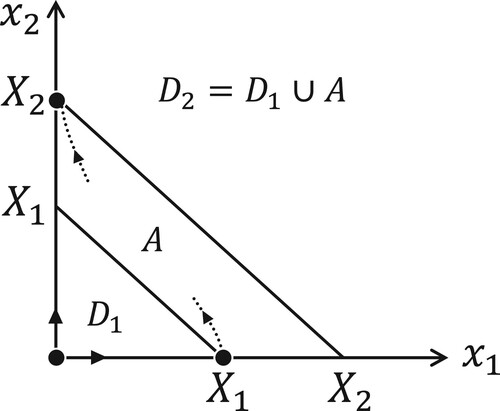
Figure 1. The phase plane $(x_1,x_2)$ of system (1(1) $\{\begin{array}{l}{x}_1(n+1)=x_1(n)\{(1-\eta )\exp (\lambda -x_1(n)-x_2(n))+\eta s\}\\ x_2(n+1)=x_2(n)\exp (\lambda -x_1(n)-x_2(n)),\end{array}$(1) ). The set $D_1$ is a proper subset of $D_2$. Species 1 is dominated by species 2. The unstable manifold of $(X_1,0)$ and the stable manifold of $(0,X_2)$ have nonempty intersections with the interior of ${\mathbb{R}}_{+}^2$.

Let $J(x_1,x_2)$ be the Jacobi matrix of system (1(1) $\{\begin{array}{l}{x}_1(n+1)=x_1(n)\{(1-\eta )\exp (\lambda -x_1(n)-x_2(n))+\eta s\}\\ x_2(n+1)=x_2(n)\exp (\lambda -x_1(n)-x_2(n)),\end{array}$(1) ) evaluated at $(x_1,x_2)$. Then $J(0,0)$ has the eigenvalues $(1-\eta )e^{\lambda }+\eta s$ and $e^{\lambda }$, both of which are larger than one for all $\eta >0$ sufficiently small since $\lambda >0$. Thus, the origin is a source for all $\eta >0$ sufficiently small. $J(X_1,0)$ has the eigenvalues $1-(1-s\eta )X_1$ and $\exp (\lambda -X_1)=\exp (X_2-X_1)>1$. The former eigenvalue determines the stability of the fixed point $X_1$ of the map $f_1$ defined in the previous section. Note that $X_1$ is destabilized at $\lambda =\frac{2}{1-\eta }+\ln \frac{1-\eta s}{1-\eta }$ as λ is increased. The latter eigenvalue is transversal in the sense that it has an eigenvector transversal to the $x_1$-axis. Thus the unstable manifold of $(X_1,0)$ always has a nonempty intersection with the interior of ${\mathbb{R}}_{+}^2$. $J(0,X_2)$ has the eigenvalues $1-X_2$ and $(1-\eta )\exp (\lambda -X_2)+\eta s=1-\eta (1-s)<1$. The former eigenvalue determines the stability of the fixed point $X_2$ of the map $f_2$ defined in the previous section. Note that $X_2$ is destabilized at $\lambda =2$ as λ is increased. The latter eigenvalue is transversal. Thus the stable manifold of $(0,X_2)$ always has a nonempty intersection with the interior of ${\mathbb{R}}_{+}^2$. Figure 1 summarizes some of the above results.

4. Stability of boundary 2-cycles

Concerning the stability of boundary 2-cycles of system (1(1) $\{\begin{array}{l}{x}_1(n+1)=x_1(n)\{(1-\eta )\exp (\lambda -x_1(n)-x_2(n))+\eta s\}\\ x_2(n+1)=x_2(n)\exp (\lambda -x_1(n)-x_2(n)),\end{array}$(1) ), we obtain the following theorem.

Theorem 4.1

If $\lambda >2$, then system (1(1) $\{\begin{array}{l}{x}_1(n+1)=x_1(n)\{(1-\eta )\exp (\lambda -x_1(n)-x_2(n))+\eta s\}\\ x_2(n+1)=x_2(n)\exp (\lambda -x_1(n)-x_2(n)),\end{array}$(1) ) with $\eta >0$ sufficiently small has the 2-cycles ${\mathcal{P}}_1:=\{(P_1,0),(P_1^{\ast },0)\}$ and ${\mathcal{P}}_2:=\{(0,P_2),(0,P_2^{\ast })\}$.

(a)	If $2<\lambda <{\lambda }_2$ and $\lambda <h({\cosh }^{-1}\frac{1}{s})$, then ${\mathcal{P}}_1$ is a saddle with an unstable manifold that intersects the interior of ${\mathbb{R}}_{+}^2$ and ${\mathcal{P}}_2$ is a sink whenever $\eta >0$ is sufficiently small.
(b)	If $2<\lambda <{\lambda }_2$ and $\lambda >h({\cosh }^{-1}\frac{1}{s})$, then ${\mathcal{P}}_1$ is a sink and ${\mathcal{P}}_2$ is a saddle with an unstable manifold that intersects the interior of ${\mathbb{R}}_{+}^2$ whenever $\eta >0$ is sufficiently small.
(c)	If $\lambda >2$ and $\lambda <h({\cosh }^{-1}\frac{1}{s})$, then ${\mathcal{P}}_1$ is a source and ${\mathcal{P}}_2$ is a saddle with a stable manifold that intersects the interior of ${\mathbb{R}}_{+}^2$ whenever $\eta >0$ is sufficiently small.
(d)	If $\lambda >2$ and $\lambda >h({\cosh }^{-1}\frac{1}{s})$, then ${\mathcal{P}}_1$ is a saddle with a stable manifold that intersects the interior of ${\mathbb{R}}_{+}^2$ and ${\mathcal{P}}_2$ is a source whenever $\eta >0$ is sufficiently small.

Proof.

Since system (1(1) $\{\begin{array}{l}{x}_1(n+1)=x_1(n)\{(1-\eta )\exp (\lambda -x_1(n)-x_2(n))+\eta s\}\\ x_2(n+1)=x_2(n)\exp (\lambda -x_1(n)-x_2(n)),\end{array}$(1) ) is reduced to the Ricker map on the $x_2$-axis, system (1(1) $\{\begin{array}{l}{x}_1(n+1)=x_1(n)\{(1-\eta )\exp (\lambda -x_1(n)-x_2(n))+\eta s\}\\ x_2(n+1)=x_2(n)\exp (\lambda -x_1(n)-x_2(n)),\end{array}$(1) ) has the 2-cycle ${\mathcal{P}}_2=\{(0,P_2),(0,P_2^{\ast })\}$ for all $\eta >0$ if $\lambda >2$. Recall that $J(x_1,x_2)$ denotes the Jacobi matrix of system (1(1) $\{\begin{array}{l}{x}_1(n+1)=x_1(n)\{(1-\eta )\exp (\lambda -x_1(n)-x_2(n))+\eta s\}\\ x_2(n+1)=x_2(n)\exp (\lambda -x_1(n)-x_2(n)),\end{array}$(1) ) evaluated at $(x_1,x_2)$. Then the Jacobi matrix of the second iterate of system (1(1) $\{\begin{array}{l}{x}_1(n+1)=x_1(n)\{(1-\eta )\exp (\lambda -x_1(n)-x_2(n))+\eta s\}\\ x_2(n+1)=x_2(n)\exp (\lambda -x_1(n)-x_2(n)),\end{array}$(1) ) evaluated at ${\mathcal{P}}_2$ is given by $J(0,P_2)J(0,P_2^{\ast })$. This matrix has the eigenvalues (10) $f_2^{\prime }(P_2)f_2^{\prime }(P_2^{\ast })\mathrm{and}\{(1-\eta )\exp (\lambda -P_2)+\eta s\}\{(1-\eta )\exp (\lambda -P_2^{\ast })+\eta s\}.$(10) As mentioned in Section 2, the absolute value of the former eigenvalue is less than one if $\lambda \in (2,{\lambda }_2)$. The latter eigenvalue takes the form $1+[-2+s\{\exp (\lambda -P_2)+\exp (\lambda -P_2^{\ast })\}]\eta +O({\eta }^2).$Using (5(5) $P_2=\frac{2\xi }{1-e^{-\xi }}=\lambda +\xi ,P_2^{\ast }=\frac{2\xi e^{-\xi }}{1-e^{-\xi }}=\lambda -\xi ,$(5) ), we find that the absolute value of this eigenvalue is less (resp. larger) than one for all $\eta >0$ sufficiently small if $s<\frac{1}{\cosh \xi }$ (resp. $s>\frac{1}{\cosh \xi }$). Therefore, the case where the 2-cycle ${\mathcal{P}}_2$ is hyperbolic can be divided into four cases: (a) $2<\lambda <{\lambda }_2$ and $s<\frac{1}{\cosh \xi }$, (b) $2<\lambda <{\lambda }_2$ and $s>\frac{1}{\cosh \xi }$, (c) $\lambda >{\lambda }_2$ and $s<\frac{1}{\cosh \xi }$, and (d) $\lambda >{\lambda }_2$ and $s>\frac{1}{\cosh \xi }$. The 2-cycle ${\mathcal{P}}_2$ is a sink in case (a), a saddle in cases (b) and (c), and a source in case (d). Furthermore, we find that ${\mathcal{P}}_2$ has an unstable manifold that intersects the interior of ${\mathbb{R}}_{+}^2$ in case (b) since the latter eigenvalue is transversal. Similarly, we find that ${\mathcal{P}}_2$ has a stable manifold that intersects the interior of ${\mathbb{R}}_{+}^2$ in case (c).

By Lemma 2.1, system (1(1) $\{\begin{array}{l}{x}_1(n+1)=x_1(n)\{(1-\eta )\exp (\lambda -x_1(n)-x_2(n))+\eta s\}\\ x_2(n+1)=x_2(n)\exp (\lambda -x_1(n)-x_2(n)),\end{array}$(1) ) has the 2-cycle ${\mathcal{P}}_1=\{(P_1,0),(P_1^{\ast },0)\}$ on the $x_1$-axis for all $\eta >0$ sufficiently small if $\lambda >2$. The Jacobi matrix of the second iterate of system (1(1) $\{\begin{array}{l}{x}_1(n+1)=x_1(n)\{(1-\eta )\exp (\lambda -x_1(n)-x_2(n))+\eta s\}\\ x_2(n+1)=x_2(n)\exp (\lambda -x_1(n)-x_2(n)),\end{array}$(1) ) evaluated at ${\mathcal{P}}_1$ is given by $J(P_1,0)J(P_1^{\ast },0)$. This matrix has the eigenvalues (11) $f_1^{\prime }(P_1)f_1^{\prime }(P_1^{\ast })\mathrm{and}\exp (\lambda -P_1)\exp (\lambda -P_1^{\ast }).$(11) As shown in Lemma 2.1, the absolute value of the former eigenvalue is less than one for all $\eta >0$ sufficiently small if $\lambda \in (2,{\lambda }_2)$. Equation (5(5) $P_2=\frac{2\xi }{1-e^{-\xi }}=\lambda +\xi ,P_2^{\ast }=\frac{2\xi e^{-\xi }}{1-e^{-\xi }}=\lambda -\xi ,$(5) ) reduces the latter eigenvalue into $\exp (2\lambda -P_2-P_2^{\ast }-2(s\cosh \xi -1)\eta +O({\eta }^2)),$whose absolute value is less (resp. larger) than one for all $\eta >0$ sufficiently small if $s>\frac{1}{\cosh \xi }$ (reps. $s<\frac{1}{\cosh \xi }$) since $2\lambda =P_2+P_2^{\ast }$. Therefore, the case where the 2-cycle ${\mathcal{P}}_1$ is hyperbolic can be divided into four cases (a), (b), (c), and (d) as above. The 2-cycle ${\mathcal{P}}_1$ is a saddle in case (a), a sink in cases (b), a source in case (c), and a saddle in case (d). Furthermore, we find that ${\mathcal{P}}_1$ has an unstable manifold that intersects the interior of ${\mathbb{R}}_{+}^2$ in case (a) since the latter eigenvalue is transversal. Similarly, we find that ${\mathcal{P}}_1$ has a stable manifold that intersects the interior of ${\mathbb{R}}_{+}^2$ in case (d).

The inequalities $s<\frac{1}{\cosh \xi }$ and $s>\frac{1}{\cosh \xi }$ can be rewritten as follows: (12) $s<\frac{1}{\cosh \xi }\iff \lambda <h({\cosh }^{-1}\frac{1}{s})\mathrm{and}s>\frac{1}{\cosh \xi }\iff \lambda >h({\cosh }^{-1}\frac{1}{s}).$(12) In fact, since the function $h(x)$ defined by (6(6) $h(\xi ):=\xi \frac{1+e^{-\xi }}{1-e^{-\xi }}=\frac{\xi }{\tanh \left(\frac{\xi }{2}\right)}$(6) ) is strictly increasing for x>0, $\lambda =h(\xi )<h({\cosh }^{-1}\frac{1}{s})$ if and only if $\xi <{\cosh }^{-1}\frac{1}{s}$ and $\lambda =h(\xi )>h({\cosh }^{-1}\frac{1}{s})$ if and only if $\xi >{\cosh }^{-1}\frac{1}{s}$. Thus we obtain (12(12) $s<\frac{1}{\cosh \xi }\iff \lambda <h({\cosh }^{-1}\frac{1}{s})\mathrm{and}s>\frac{1}{\cosh \xi }\iff \lambda >h({\cosh }^{-1}\frac{1}{s}).$(12) ).

Note that ${\mathcal{P}}_1$ is asymptotically stable for all $\eta >0$ sufficiently small if $2<\lambda <{\lambda }_2$ and $\lambda >h({\cosh }^{-1}\frac{1}{s})$ and is unstable for all $\eta >0$ sufficiently small if either $\lambda >{\lambda }_2$ or $\lambda <h({\cosh }^{-1}\frac{1}{s})$ and ${\mathcal{P}}_2$ is asymptotically stable for all $\eta >0$ sufficiently small if $2<\lambda <{\lambda }_2$ and $\lambda <h({\cosh }^{-1}\frac{1}{s})$ and is unstable for all $\eta >0$ sufficiently small if either $\lambda >{\lambda }_2$ or $\lambda >h({\cosh }^{-1}\frac{1}{s})$.

The above result is summarized in Table 1. The table shows that each boundary fixed point or 2-cycle has the indicated stability if they satisfy the indicated parameter conditions. Note, however, that the fixed point $(X_1,0)$ and the 2-cycles ${\mathcal{P}}_1$ and ${\mathcal{P}}_2$ have the indicated stability if $\eta >0$ is sufficiently small. Since ${\cosh }^{-1}x=\ln (x+\sqrt{x^2-1})$, we have the following expression: $h({\cosh }^{-1}\frac{1}{s})=h(\ln (\frac{1}{s}+\sqrt{\frac{1}{s^2}-1})).$Figure 2 shows the parameter plane demarcated with the stability of the boundary fixed points and the boundary 2-cycles of system (1(1) $\{\begin{array}{l}{x}_1(n+1)=x_1(n)\{(1-\eta )\exp (\lambda -x_1(n)-x_2(n))+\eta s\}\\ x_2(n+1)=x_2(n)\exp (\lambda -x_1(n)-x_2(n)),\end{array}$(1) ) with $\eta \approx 0$.

Table 1. Stability of the boundary fixed points and the boundary 2-cycles of system (1(1) $\{\begin{array}{l}{x}_1(n+1)=x_1(n)\{(1-\eta )\exp (\lambda -x_1(n)-x_2(n))+\eta s\}\\ x_2(n+1)=x_2(n)\exp (\lambda -x_1(n)-x_2(n)),\end{array}$(1) ).

	$0<\lambda <2$	$2<\lambda <{\lambda }_2$		${\lambda }_2<\lambda$
		$s<\frac{1}{\cosh \xi }$	$s>\frac{1}{\cosh \xi }$
$(0,0)$	U	U	U	U
$(X_1,0)$	U	U	U	U
$(0,X_2)$	AS	U	U	U
$\{(P_1,0),(P_1^{\ast },0)\}$	–	U	AS	U
$\{(0,P_2),(0,P_2^{\ast })\}$	–	AS	U	U

Note: AS and U stand for asymptotically stable and unstable, respectively.

Figure 2. The parameter plane $(\lambda ,s)$ of system (1(1) $\{\begin{array}{l}{x}_1(n+1)=x_1(n)\{(1-\eta )\exp (\lambda -x_1(n)-x_2(n))+\eta s\}\\ x_2(n+1)=x_2(n)\exp (\lambda -x_1(n)-x_2(n)),\end{array}$(1) ) with $\eta \approx 0$. In regions A, B, and C, $(0,X_2)$, ${\mathcal{P}}_2$, and ${\mathcal{P}}_1$ are asymptotically stable, respectively. There are no stable fixed points nor stable 2-cycles on the boundary of ${\mathbb{R}}_{+}^2$ if $\lambda >{\lambda }_2$.

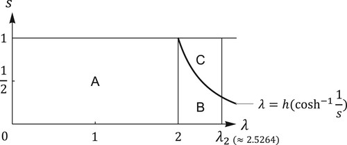
Figure 3. The parameter plane $(\lambda ,s)$ of system (1(1) $\{\begin{array}{l}{x}_1(n+1)=x_1(n)\{(1-\eta )\exp (\lambda -x_1(n)-x_2(n))+\eta s\}\\ x_2(n+1)=x_2(n)\exp (\lambda -x_1(n)-x_2(n)),\end{array}$(1) ). The green and red regions correspond to the region B and C in Figure 2, respectively. In the yellow region, both ${\mathcal{P}}_1$ and ${\mathcal{P}}_2$ have unstable transversal eigenvalues, i.e. both species can mutually invade at the boundary 2-cycles. On the left and right panels, $\eta =0.01$ and $\eta =0.1$, respectively.

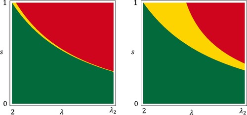
From Table 1, we find that if $(\lambda ,s)$ belongs to the region C of Figure 2 and $\eta \approx 0$, then the monoculture system of species 2 is settled in ${\mathcal{P}}_2$ and cannot prevent invasion of species 1 while the monoculture system of species 1 is settled in ${\mathcal{P}}_1$ and can prevent invasion of species 2. This implies that delayed reproduction can be adaptive if a fraction η of juveniles delays the initiation of reproduction and both the juvenile survival probability and the amplitude of population fluctuation are sufficiently large. Although we do not have a mathematical estimate how small η should be, the numerical result shown in Figure 3 suggests that the region C persists even if $\eta =0.1$. In Figure 3, the eigenvalues shown in (10(10) $f_2^{\prime }(P_2)f_2^{\prime }(P_2^{\ast })\mathrm{and}\{(1-\eta )\exp (\lambda -P_2)+\eta s\}\{(1-\eta )\exp (\lambda -P_2^{\ast })+\eta s\}.$(10) ) and (11(11) $f_1^{\prime }(P_1)f_1^{\prime }(P_1^{\ast })\mathrm{and}\exp (\lambda -P_1)\exp (\lambda -P_1^{\ast }).$(11) ) are numerically calculated. In the yellow region of Figure 3, two species can mutually invade each other at ${\mathcal{P}}_1$ and ${\mathcal{P}}_2$ and coexist. We see that the yellow region gets larger as η increases.

5. Global dynamics

In this section, we examine the global dynamics of system (1(1) $\{\begin{array}{l}{x}_1(n+1)=x_1(n)\{(1-\eta )\exp (\lambda -x_1(n)-x_2(n))+\eta s\}\\ x_2(n+1)=x_2(n)\exp (\lambda -x_1(n)-x_2(n)),\end{array}$(1) ) analytically and numerically. First, we show that it is unlikely that system (1(1) $\{\begin{array}{l}{x}_1(n+1)=x_1(n)\{(1-\eta )\exp (\lambda -x_1(n)-x_2(n))+\eta s\}\\ x_2(n+1)=x_2(n)\exp (\lambda -x_1(n)-x_2(n)),\end{array}$(1) ) has a positive 2-cycle as long as $\eta \approx 0$.

Theorem 5.1

Suppose that either $\lambda \le 2$ or $\lambda >2$ and $\lambda \ne h({\cosh }^{-1}\frac{1}{s})$. Then system (1(1) $\{\begin{array}{l}{x}_1(n+1)=x_1(n)\{(1-\eta )\exp (\lambda -x_1(n)-x_2(n))+\eta s\}\\ x_2(n+1)=x_2(n)\exp (\lambda -x_1(n)-x_2(n)),\end{array}$(1) ) has no positive 2-cycles for all $\eta >0$ sufficiently small.

Proof.

Let $\{(x_1,x_2),(x_1^{\ast },x_2^{\ast })\}$ be a positive 2-cycle of system (1(1) $\{\begin{array}{l}{x}_1(n+1)=x_1(n)\{(1-\eta )\exp (\lambda -x_1(n)-x_2(n))+\eta s\}\\ x_2(n+1)=x_2(n)\exp (\lambda -x_1(n)-x_2(n)),\end{array}$(1) ). Then it satisfies the system of equations (13) $\{\begin{array}{l}1=\{(1-\eta )\exp (\lambda -x_1-x_2)+\eta s\}\{(1-\eta )\exp (\lambda -x_1^{\ast }-x_2^{\ast })+\eta s\}\\ 2\lambda =x_1+x_2+x_1^{\ast }+x_2^{\ast },\end{array}$(13) where (14) $x_1^{\ast }=x_1\{(1-\eta )\exp (\lambda -x_1-x_2)+\eta s\}\mathrm{and}{x}_2^{\ast }=x_2\exp (\lambda -x_1-s_2).$(14) By using the second equation of (13(13) $\{\begin{array}{l}1=\{(1-\eta )\exp (\lambda -x_1-x_2)+\eta s\}\{(1-\eta )\exp (\lambda -x_1^{\ast }-x_2^{\ast })+\eta s\}\\ 2\lambda =x_1+x_2+x_1^{\ast }+x_2^{\ast },\end{array}$(13) ), we can remove $x_1^{\ast }+x_2^{\ast }$ from the first equation of (13(13) $\{\begin{array}{l}1=\{(1-\eta )\exp (\lambda -x_1-x_2)+\eta s\}\{(1-\eta )\exp (\lambda -x_1^{\ast }-x_2^{\ast })+\eta s\}\\ 2\lambda =x_1+x_2+x_1^{\ast }+x_2^{\ast },\end{array}$(13) ) as follows: (15) $(1-\eta )s{Y}^2-(2-\eta -\eta s^2)Y+(1-\eta )s=0,$(15) where (16) $Y=\exp (\lambda -(x_1+x_2)).$(16) Since $s,\eta \in (0,1)$, the quadratic Equation (15(15) $(1-\eta )s{Y}^2-(2-\eta -\eta s^2)Y+(1-\eta )s=0,$(15) ) has the two positive distinct real roots $Y_{\pm }(s,\eta ):=\frac{2-\eta -\eta s^2\pm \sqrt{(1-s^2)\{{\eta }^2(1-s^2)+4(1-\eta )\}}}{2(1-\eta )s}.$By using (14(14) $x_1^{\ast }=x_1\{(1-\eta )\exp (\lambda -x_1-x_2)+\eta s\}\mathrm{and}{x}_2^{\ast }=x_2\exp (\lambda -x_1-s_2).$(14) ) and (16(16) $Y=\exp (\lambda -(x_1+x_2)).$(16) ), we can remove $x_1+x_2$ from the second equation of (13(13) $\{\begin{array}{l}1=\{(1-\eta )\exp (\lambda -x_1-x_2)+\eta s\}\{(1-\eta )\exp (\lambda -x_1^{\ast }-x_2^{\ast })+\eta s\}\\ 2\lambda =x_1+x_2+x_1^{\ast }+x_2^{\ast },\end{array}$(13) ) as follows: $2\lambda =(\lambda -\ln Y)+x_1\{(1-\eta )Y+\eta s\}+x_{2}Y.$Thus, $x_1$ and $x_2$ must satisfy the following system of linear equations: (17) $\{\begin{array}{l}\lambda -\ln Y_{\pm }(s,\eta )=x_1+x_2,\\ \lambda +\ln Y_{\pm }(s,\eta )=\{(1-\eta )Y_{\pm }(s,\eta )+\eta s\}{x}_1+Y_{\pm }(s,\eta )x_2.\end{array}$(17) Since the two equations of (17(17) $\{\begin{array}{l}\lambda -\ln Y_{\pm }(s,\eta )=x_1+x_2,\\ \lambda +\ln Y_{\pm }(s,\eta )=\{(1-\eta )Y_{\pm }(s,\eta )+\eta s\}{x}_1+Y_{\pm }(s,\eta )x_2.\end{array}$(17) ) represent parallel lines on the plane $(x_1,x_2)$ if $\eta =0$ and have negative slopes, (17(17) $\{\begin{array}{l}\lambda -\ln Y_{\pm }(s,\eta )=x_1+x_2,\\ \lambda +\ln Y_{\pm }(s,\eta )=\{(1-\eta )Y_{\pm }(s,\eta )+\eta s\}{x}_1+Y_{\pm }(s,\eta )x_2.\end{array}$(17) ) does not have positive solutions $(x_1,x_2)$ for all $\eta >0$ sufficiently small if $\lambda -\ln Y_{\pm }(s,0)\ne \frac{\lambda +\ln Y_{\pm }(s,0)}{Y_{\pm }(s,0)}.$Since $Y_{\pm }(s,0)=\frac{1}{s}\pm \sqrt{\frac{1}{s^2}-1}\ne 1$ for $s\in (0,1)$, the above condition is equivalent to $\begin{array}{rl}\lambda & \ne (\ln Y_{\pm }(s,0))\frac{1+\frac{1}{Y_{\pm }(s,0)}}{1-\frac{1}{Y_{\pm }(s,0)}}=(\ln Y_{+}(s,0))\frac{1+\frac{1}{Y_{+}(s,0)}}{1-\frac{1}{Y_{+}(s,0)}}=h(\ln Y_{+}(s,0))\\ & =h({\cosh }^{-1}\frac{1}{s}),\end{array}$where $Y_{+}(s,0)Y_{-}(s,0)=1$ is used to obtain the first equality.

Since $h({\cosh }^{-1}\frac{1}{s})$ is strictly decreasing for $s\in (0,1)$, we have $h({\cosh }^{-1}\frac{1}{s})>\underset{s\to 1^{-}}{lim}h({\cosh }^{-1}\frac{1}{s})=2$, which implies that $\lambda \ne h({\cosh }^{-1}\frac{1}{s})$ holds for all $s\in (0,1)$ if $\lambda \le 2$.

Since system (1(1) $\{\begin{array}{l}{x}_1(n+1)=x_1(n)\{(1-\eta )\exp (\lambda -x_1(n)-x_2(n))+\eta s\}\\ x_2(n+1)=x_2(n)\exp (\lambda -x_1(n)-x_2(n)),\end{array}$(1) ) has no positive fixed points, any orbit of system (1(1) $\{\begin{array}{l}{x}_1(n+1)=x_1(n)\{(1-\eta )\exp (\lambda -x_1(n)-x_2(n))+\eta s\}\\ x_2(n+1)=x_2(n)\exp (\lambda -x_1(n)-x_2(n)),\end{array}$(1) ) cannot converge to a positive point. Furthermore, by the above theorem, we see that it is unlikely that an orbit staring at a positive point converges to a positive 2-cycle if $\eta \approx 0$. Although system (1(1) $\{\begin{array}{l}{x}_1(n+1)=x_1(n)\{(1-\eta )\exp (\lambda -x_1(n)-x_2(n))+\eta s\}\\ x_2(n+1)=x_2(n)\exp (\lambda -x_1(n)-x_2(n)),\end{array}$(1) ) might have more complicated positive attractors, numerical simulations suggest that any orbit of system (1(1) $\{\begin{array}{l}{x}_1(n+1)=x_1(n)\{(1-\eta )\exp (\lambda -x_1(n)-x_2(n))+\eta s\}\\ x_2(n+1)=x_2(n)\exp (\lambda -x_1(n)-x_2(n)),\end{array}$(1) ) starting at a positive point cannot remain in a compact set bounded away from the coordinate axes as long as $\eta \approx 0$ and $(\lambda ,s)$ belongs to the region B or C of Figure 2 (see Figure 4). Figure 4 (a) shows the basin of attraction of ${\mathcal{P}}_1$ of system (1(1) $\{\begin{array}{l}{x}_1(n+1)=x_1(n)\{(1-\eta )\exp (\lambda -x_1(n)-x_2(n))+\eta s\}\\ x_2(n+1)=x_2(n)\exp (\lambda -x_1(n)-x_2(n)),\end{array}$(1) ) whose $(\lambda ,s)$ belongs to the region C of Figure 2 and $\eta =0.1$. The points in the green and yellow regions are attracted by ${\mathcal{P}}_1$. The two colours indicate whether a point is attracted by $(P_1,0)$ or $(P_1^{\ast },0)$ when looking at the orbit every other time. It is unlikely that the points on the boundaries of regions with different colours are attracted by ${\mathcal{P}}_1$. At least it is clear that the fixed point $(0,X_2)$ has a stable manifold that intersects with the interior of ${\mathbb{R}}_{+}^2$. Therefore, the points on the boundaries of two different colours seems to be attracted by $(0,X_2)$. 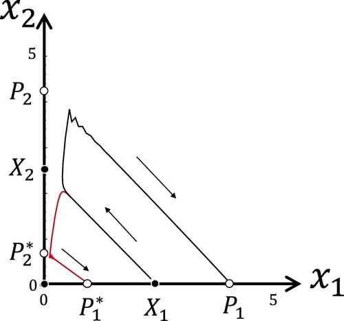Figure 5 shows a single forward orbit of system (1(1) $\{\begin{array}{l}{x}_1(n+1)=x_1(n)\{(1-\eta )\exp (\lambda -x_1(n)-x_2(n))+\eta s\}\\ x_2(n+1)=x_2(n)\exp (\lambda -x_1(n)-x_2(n)),\end{array}$(1) ) with the same parameters as in Figure 4(a). The orbit starts in a neighbourhood of $(X_1,0)$. Since the fixed point $(X_1,0)$ is unstable, the orbit leaves its neighbourhood and approaches ${\mathcal{P}}_1$ after passing by the fixed point $(0,X_2)$. This behaviour suggests that there is a heteroclinic orbit from $(X_1,0)$ to $(0,X_2)$. Figure 4 (b) shows the basin of attraction of ${\mathcal{P}}_2$ of system (1(1) $\{\begin{array}{l}{x}_1(n+1)=x_1(n)\{(1-\eta )\exp (\lambda -x_1(n)-x_2(n))+\eta s\}\\ x_2(n+1)=x_2(n)\exp (\lambda -x_1(n)-x_2(n)),\end{array}$(1) ) whose $(\lambda ,s)$ belongs to the region B of Figure 2 and $\eta =0.1$.

Figure 4. The basins of attraction of the boundary 2-cycles of system (1(1) $\{\begin{array}{l}{x}_1(n+1)=x_1(n)\{(1-\eta )\exp (\lambda -x_1(n)-x_2(n))+\eta s\}\\ x_2(n+1)=x_2(n)\exp (\lambda -x_1(n)-x_2(n)),\end{array}$(1) ). The vertical and horizontal axes are $x_1$ and $x_2$, respectively. (a) The points in the green and yellow regions are attracted by $(P_1,0)$ and $(P_1^{\ast },0)$, respectively, under the second iterate of system (1(1) $\{\begin{array}{l}{x}_1(n+1)=x_1(n)\{(1-\eta )\exp (\lambda -x_1(n)-x_2(n))+\eta s\}\\ x_2(n+1)=x_2(n)\exp (\lambda -x_1(n)-x_2(n)),\end{array}$(1) ). The parameters are $\lambda =2.5$, s = 0.6, and $\eta =0.1$. (b) The points in the black and red regions are attracted by $(0,P_2)$ and $(0,P_2^{\ast })$, respectively, under the second iterate of system (1(1) $\{\begin{array}{l}{x}_1(n+1)=x_1(n)\{(1-\eta )\exp (\lambda -x_1(n)-x_2(n))+\eta s\}\\ x_2(n+1)=x_2(n)\exp (\lambda -x_1(n)-x_2(n)),\end{array}$(1) ). The parameters are $\lambda =2.5$, s = 0.1, and $\eta =0.1$.

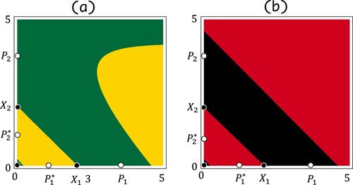
Figure 5. A single forward orbit of system (1(1) $\{\begin{array}{l}{x}_1(n+1)=x_1(n)\{(1-\eta )\exp (\lambda -x_1(n)-x_2(n))+\eta s\}\\ x_2(n+1)=x_2(n)\exp (\lambda -x_1(n)-x_2(n)),\end{array}$(1) ). The points of the orbit are connected with black and red lines if they are points of $2n$th and 2n + 1th iteration, respectively. The parameters are the same as in Figure 4 (a).

6. Concluding remarks

We studied the dynamics of system (1(1) $\{\begin{array}{l}{x}_1(n+1)=x_1(n)\{(1-\eta )\exp (\lambda -x_1(n)-x_2(n))+\eta s\}\\ x_2(n+1)=x_2(n)\exp (\lambda -x_1(n)-x_2(n)),\end{array}$(1) ), which describes competition between two semelparous species. One species is assumed to have a fraction η of individuals who delay the initiation of reproduction while the other species is assumed to reproduce every unit time. All other properties of these two species are assumed to be identical. Under the assumption $\eta \approx 0$, we analytically obtained a parameter plane $(\lambda ,s)$ demarcated with the advantage of these two species (see Figure 2). The parameter plane shows that delayed reproduction can be adaptive if both juvenile survival probability and amplitude of population fluctuation are sufficiently large as long as a fraction of juveniles delays reproduction.

System (1(1) $\{\begin{array}{l}{x}_1(n+1)=x_1(n)\{(1-\eta )\exp (\lambda -x_1(n)-x_2(n))+\eta s\}\\ x_2(n+1)=x_2(n)\exp (\lambda -x_1(n)-x_2(n)),\end{array}$(1) ) is a special case of system (2(2) $\{\begin{array}{l}{x}_1(n+1)=x_1(n)\exp (r_1-k_1(x_1(n)+x_2(n)))+\beta x_1(n)\\ x_2(n+1)=x_2(n)\exp (r_2-k_2(x_1(n)+x_2(n))),\end{array}$(2) ) studied by Yakubu [19], who considers competition between two semelparous species and assumes that one species is endangered and planted (or stocked) with a constant rate. In this interpretation, system (1(1) $\{\begin{array}{l}{x}_1(n+1)=x_1(n)\{(1-\eta )\exp (\lambda -x_1(n)-x_2(n))+\eta s\}\\ x_2(n+1)=x_2(n)\exp (\lambda -x_1(n)-x_2(n)),\end{array}$(1) ) considers the case where the endangered species whose fertility is reduced by the proportion η in compared with the competitor is planted (or stocked) at a rate $\eta s$ (0<s<1). Our result shows that if the population is fluctuating, then the endangered species can be saved by poor planting not covering the reduction of fertility. Note that a similar interpretation is possible if species 1 is considered iteroparous and species 2 semelparous (see [1,7]).

By applying the general result of Franke and Yakubu [5, Theorem 6.1] to system (1(1) $\{\begin{array}{l}{x}_1(n+1)=x_1(n)\{(1-\eta )\exp (\lambda -x_1(n)-x_2(n))+\eta s\}\\ x_2(n+1)=x_2(n)\exp (\lambda -x_1(n)-x_2(n)),\end{array}$(1) ), we can show that if the fixed points $(X_1,0)$ and $(0,X_2)$ are global attractors within each positive coordinate axis, then $(0,X_2)$ attracts all points in the interior of ${\mathbb{R}}_{+}^2$ since species 1 is dominated by species 2. However, as we showed, if the coordinate axes have the 2-cycles ${\mathcal{P}}_1$ and ${\mathcal{P}}_2$, then both ${\mathcal{P}}_1$ and ${\mathcal{P}}_2$ can be asymptotically stable in system (1(1) $\{\begin{array}{l}{x}_1(n+1)=x_1(n)\{(1-\eta )\exp (\lambda -x_1(n)-x_2(n))+\eta s\}\\ x_2(n+1)=x_2(n)\exp (\lambda -x_1(n)-x_2(n)),\end{array}$(1) ) with $\eta \approx 0$. Note, however, that a stable boundary 2-cycle cannot attract all points in the interior of ${\mathbb{R}}_{+}^2$ since $(0,X_2)$ always has a stable manifold that intersects with the interior of ${\mathbb{R}}_{+}^2$. Our numerical simulation suggests that heteroclinic orbits from $(X_1,0)$ to $(0,X_2)$ belong to the stable manifold. Furthermore, as shown by Kang and Smith [13], who examines a variant of system (2(2) $\{\begin{array}{l}{x}_1(n+1)=x_1(n)\exp (r_1-k_1(x_1(n)+x_2(n)))+\beta x_1(n)\\ x_2(n+1)=x_2(n)\exp (r_2-k_2(x_1(n)+x_2(n))),\end{array}$(2) ), it is likely that all the pre-images of the closure of the union of all the heteroclinic orbits also cannot be attracted by ${\mathcal{P}}_1$ (see also [12]). It is a future problem to reveal the basin of attraction of ${\mathcal{P}}_1$ when it is asymptotically stable. It is worth noting that riddled basins of attraction are observed in a slightly more general system that includes system (2(2) $\{\begin{array}{l}{x}_1(n+1)=x_1(n)\exp (r_1-k_1(x_1(n)+x_2(n)))+\beta x_1(n)\\ x_2(n+1)=x_2(n)\exp (r_2-k_2(x_1(n)+x_2(n))),\end{array}$(2) ) as a special case [2] and intermingled basins of attraction are constructed in a certain discrete-time competition model [9].

Disclosure statement

No potential conflict of interest was reported by the author(s).

Additional information

Funding

This work was supported by JSPS KAKENHI [grant number 20K03735], Japan.

References

- M. Bulmer, Theoretical Evolutionary Ecology, Sinauer Associates, Sunderland, Massachusetts, 1994.
- O. de Feo and R. Ferriere, Bifurcation analysis of population invasion: On-off intermittency and basin riddling, Internat. J. Bifur. Chaos Appl. Sci. Engrg. 10(2) (2000), pp. 443–452.
- S. Elaydi and R.J. Sacker, Basin of attraction of periodic orbits of maps on the real line, J. Differ. Equ. Appl. 10(10) (2004), pp. 881–888.
- S. Elaydi and A.-A. Yakubu, Global stability of cycles: Lotka-Volterra competition model with stocking, J. Differ. Equ. Appl. 8(6) (2002), pp. 537–549.
- J.E. Franke and A.-A. Yakubu, Global attractors in competitive systems, Nonlinear Anal. 16(2) (1991), pp. 111–129.
- J.E. Franke and A.-A. Yakubu, Mutual exclusion versus coexistence for discrete competitive systems, J. Math. Bio. 30(2) (1991), pp. 161–168.
- M. Gatto, The evolutionary optimality of oscillatory and chaotic dynamics in simple population models, Theor. Popul. Biol. 43(3) (1993), pp. 310–336.
- M. Hassell and H.N. Comins, Discrete time models for two-species competition, Theor. Popul. Biol. 9(2) (1976), pp. 202–221.
- F. Hofbauer, J. Hofbauer, P. Raith, and T. Steinberger, Intermingled basins in a two species system, J. Math. Bio. 49(3) (2004), pp. 293–309.
- J. Hofbauer, V. Hutson, and W. Jansen, Coexistence for systems governed by difference equations of lotka-volterra type, J. Math. Bio. 25(5) (1987), pp. 553–570.
- H. Jiang and T.D. Rogers, The discrete dynamics of symmetric competition in the plane, J. Math. Bio. 25(6) (1987), pp. 573–596.
- Y. Kang, Pre-images of invariant sets of a discrete-time two-species competition model, J. Differ. Equ. Appl. 18(10) (2011), pp. 1709–1733.
- Y. Kang and H. Smith, Global dynamics of a discrete two-species Lottery-Ricker competition model, J. Biol. Dyn. 6(2) (2012), pp. 358–376.
- R. Kon, Convex dominates concave: An exclusion principle in discrete-time Kolmogorov systems, Proc. Amer. Math. Soc. 134(10) (2006), pp. 3025–3034.
- R. Luís, S. Elaydi, and H. Oliveira, Stability of a Ricker-type competition model and the competitive exclusion principle, J. Biol. Dyn. 5(6) (2011), pp. 636–660.
- R.M. May and G.F. Oster, Bifurcations and dynamic complexity in simple ecological models, Am. Nat. 110(974) (1976), pp. 573–599.
- S.D. Mylius and O. Diekmann, The resident strikes back: Invader-induced switching of resident attractor, J. Theoret. Biol. 211(4) (2001), pp. 297–311.
- S. Tuljapurkar, Delayed reproduction and fitness in variable environments, Proc. Natl. Acad. Sci. USA 87(3) (1990), pp. 1139–1143.
- A.-A. Yakubu, The effects of planting and harvesting on endangered species in discrete competitive systems, Math. Biosc. 126(1) (1995), pp. 1–20.
- A.-A. Yakubu, A discrete competition system with planting, J. Differ. Equ. Appl. 4(2) (1998), pp. 213–214.