
 ?Mathematical formulae have been encoded as MathML and are displayed in this HTML version using MathJax in order to improve their display. Uncheck the box to turn MathJax off. This feature requires Javascript. Click on a formula to zoom.
Abstract
In this paper, we formulate a population suppression model and a population replacement model with periodic impulsive releases of Nilaparvata lugens infected with wStri. The conditions for the stability of wild--eradication periodic solution of two systems are obtained by applying the Floquet theorem and comparison theorem. And the sufficient conditions for the persistence in the mean of wild
are also given. In addition, the sufficient conditions for the extinction and persistence of the wild
in the subsystem without wLug are also obtained. Finally, we give numerical analysis which shows that increasing the release amount or decreasing the release period are beneficial for controlling the wild
, and the efficiency of population replacement strategy in controlling wild populations is higher than that of population suppression strategy under the same release conditions.
1. Introduction
Nilaparvata lugens (N. lugens) is a monophagous pest, which can only feed and reproduce on rice and common wild rice. It is the most destructive pest on rice in many Asian countries by sucking rice phloem sap and transmitting rice ragged stunt virus () [Citation1,Citation2]. Few feasible control strategies are obtainable because of the evolution of high levels of insecticide resistance, and new environmentally friendly methods are urgently needed [Citation3]. In recent studies, disease control methods based on artificial Wolbachia infection to inhibit mosquito vector-borne pathogens have been applied [Citation4,Citation5]. Scientists are currently working on similar methods for controlling agricultural pests [Citation6].
Nilaparvata lugens can be naturally infected by Wolbachia strain wLug, which lacks the ability to induce cytoplasmic incompatibility () [Citation7]. Many experimental results show that the
infected with wLug has stronger reproductive ability than the uninfected
, and show imperfect maternal transmission characteristics [Citation6,Citation8,Citation9]. Fortunately, Gong et al. [Citation6] successfully developed a stable artificial Wolbachia infection of
by introducing the Wolbachia strain wStri from
host into
. The results [Citation6] showed that
infected with wStri maintained perfect maternal transmission and induced moderately high levels of CI. When the wStri-infected males mated with either uninfected or the wLug-infected females, the mean hatch rates per female were
and
, respectively. The results of Gong et al. [Citation6] lay a foundation for future experiments on paddy fields.
In order to theoretically study the interaction mechanism between infected with wStri and wild
population, Liu and Zhou [Citation10] proposed and studied a Wolbachia spreading dynamics model in
with two strains, and obtained sufficient conditions for the
infected with wStri to invade wild
successfully. But the authors did not address when and how many
infected with wStri is released to suppress or replace wild
, so studying the release of wStri-infected
to control wild
for future field trials with wStri is biologically significant. Currently, there are few models to study how to release the
infected Wolbachia, but many mosquito population dynamics models have been proposed and studied [Citation11–24]. Cai et al. [Citation11] considered three strategies for continuous release of sterile mosquitoes: constant release rate, release rate proportional to the wild mosquitoes and proportional release rate with saturation, and developed corresponding continuous mathematical models to study the influences of the three release strategies on the interactive dynamics of mosquitoes. In practice, continuous release of sterile mosquitoes is difficult to realize in practical applications. Huang et al. [Citation16] formulated and investigated two mathematical models with impulsive releases of sterile mosquitoes. The first model considered the periodic pulse release of sterile mosquitoes strategy and obtained a sufficient condition for the stability of the wild mosquito-eradication periodic solution. The second model considered the state-feedback pulse release strategy and proved the existence of the first-order periodic solution. In studies [Citation17–20], the authors adopted a new modelling idea that only those sexually active sterile mosquitoes were considered in the modelling process. Yu et al. [Citation19] developed and analyzed a population suppression model considering that the release period was longer than the sexual life of sterile mosquitoes. They obtained sufficient conditions for the global asymptotic stability of positive periodic solutions. Later, Zheng et al. [Citation17] considered the following situation that the release period was shorter than the sexual lifespan of sterile male mosquitoes. Li and Ai [Citation18] incorporated the maturation process of mosquito larvae to adults into their model and employed time delay to describe the maturation period of the larvae, the results showed that the delay affects the control of wild mosquitoes. In addition, some scholars considered the interaction between mosquitoes and disease transmission (such as
, Zika, etc.), and established some mathematical models to control mosquito-borne diseases [Citation23,Citation24]. For example, Taghikahani et al. [Citation23] formulated a new two-sex mathematical model for the population ecology of dengue fever and Wolbachia-infected mosquitoes, and used it to evaluate the impact of periodic release the Wolbachian-infected mosquitoes on the population-level. However, we notice from studies [Citation11–24] that most models were established around the release of male mosquitoes infected with Wolbachia (i.e. population suppression strategy), and the research on the impulsive release strategy of female mosquitoes infected with Wolbachia mostly adopts numerical simulation method.
All the models mentioned above about the release strategies of mosquitoes infected with Wolbachia also provide good help for the release of infected with wStri. Compared with the transmission characteristics of mosquitoes infected with Wolbachia, the
infected with Wolbachia has many differences. For example, the cytoplasmic incompatibility induced by the mating of male
infected with wStri with wild uninfected female
or wild female
infected with wlug is incomplete [Citation6]. To determine when is the best time to release
infected with wStri and the number of
infected with wStri per release. In 2023, Liu et al. [Citation25] established and discussed two semi-continuous models with state-feedback impulsive releases of
infected with wStri. But the authors only considered the scenario where all wild
populations were uninfected
, and there are few studies of wild
including both the wild
uninfected and infected with wLug. In this paper, we adapt the modelling idea in [Citation10] and consider the periodic impulsive release of male or female
infected with wStri into the field. And then according to the transmission characteristics of two Wolbachia strains in
, we establish two impulsive mathematical models with periodic impulsive release of
infected with wStri: population suppression model and population replacement model. We theoretically discuss the stability of the wild-
-eradication periodic solution for both models and the corresponding numerical analyses are also carried out. Furthermore, the sufficient conditions of persistence in the mean of the wild
are also established. Finally, we compare the degree of control of two periodic impulsive release strategies on the wild
within a short time.
This paper is organized as follows: In Section 2, population suppression and population replacement models with periodic impulsive release are proposed. In Section 3, we study the stability of wild- -extinction periodic solution of two models, respectively, and discuss the persistence of wild
. Then we numerically analyze the influences of release period and release amount on the control of wild
in Section 4. Finally, we present our conclusions in Section 5.
2. Model formulation
Let and
be the densities of the wild female
and male
uninfected by wLug and wStri at time t, respectively.
and
denote the densities of the wild female
and male
infected with wLug at time t, respectively.
and
represent the densities of the female
and male
infected with wStri at time t.
In order to establish the mathematical model more conveniently, we give a chart to show all possible mating patterns of according to the research conclusions of studies [Citation10,Citation25]. The fourth line of Figure shows that the males
infected with wStri
can induce higher CI level when they mate with
and
,
and
represent the CI intensity of
against
and
, respectively. The third and fourth columns of Figure indicate that the
infected with wStri has perfect maternal transmission, while the wild
infected with wLug has imperfect maternal transmission.
is the percentage of uninfected progeny produced by a wLug-infected mother. Ju et al. [Citation8] shows that Wolbachia of the wlug strain has a reproductive promoting effect on its natural host
, but wStri does not. Therefore, we assume that the uninfected
female
and the wStri-infected
female
have the same birth rate, while the birth rate of wLug-infected
female
is greater than
and
. Let a>0 be the birth rate of the uninfected
, and
is the birth rate of the wLug-infected
, where
. Moreover, we adhere to the conventional method by substituting the natural death of
population with a Logistic-like density dependent term [Citation10,Citation25]. Let
,
and
denote the decay rate constants of the uninfected
, wLug-infected
and wStri-infected
, respectively. Similar to Refs. [Citation10,Citation26,Citation27], we always assume that the proportion of individuals born male is equal to the proportion of individuals born female in this paper, that is,
,
and
.
Figure 1. All possible mating patterns of . The wild
infected with wLug has imperfect maternal transmission.
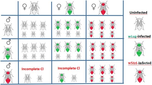
From Figure , we give all the mating patterns of , such as
come from the mating patterns
,
and
. Then the expression
denotes the probability of a female
mates with an uninfected male
,
represents the probability of a female
mates with a wLug-infected male
, and
gives the probability of incompatible crossing that a wild female
mates with a wStri-infected male
. According to the above assumptions and mating patterns of
, we propose the following two mathematical models.
2.1. Population suppression model with periodic impulsive release
To begin with, we consider the case that the wStri-infected males are released into the paddy field. It is easy to see from Figure that the mating pattern of the third column will not appear in this ecosystem. According to the mating patterns of
, we first propose the following population suppression model with periodic release:
(1)
(1) where
represents the release amount of male
infected with wStri each time. τ is the release period, and
,
,
,
.
.
Denote and
. Then model (Equation1
(1)
(1) ) can be simplified to the following model:
(2)
(2) Using a linear scaling for system (Equation2
(2)
(2) ),
and rewriting
as
, system (Equation2
(2)
(2) ) can be transmuted into
(3)
(3)
2.2. Population replacement model with periodic impulsive release
We also establish a population replacement model with periodic release. The females infected with wStri and males
infected with wStri are released into the farmland ecosystem, then the farmland ecosystem has uninfected
, wLug-infected
and wStri-infected
population. According to the mating patterns of
, a population replacement model with periodic impulsive release is given as follows:
(4)
(4) where
.
Denote ,
and
. Then model (Equation4
(4)
(4) ) can be simplified to the following model:
(5)
(5) Using a linear scaling for system (Equation5
(5)
(5) ),
and rewriting
as
, then we transmute system (Equation5
(5)
(5) ) into
(6)
(6)
3. Main results
We will study the dynamics of models (Equation3(3)
(3) ) and (Equation6
(6)
(6) ) in this section. For simplicity, denote
Definition 3.1
The population χ is said to be extinct if
.
The population χ is said to be strongly persistent in the mean if
3.1. The dynamics of model (3)
Let be the solution of system (Equation3
(3)
(3) ) with initial value
,
and
. Clearly,
is a piecewise continuous function, where
. From [Citation28], the global existence and uniqueness of solutions of system (Equation3
(3)
(3) ) is guaranteed by the smoothness properties of
, which denotes the mapping defined by the right-hand side of system (Equation3
(3)
(3) ). Denote
where
and
will be given in the following Lemmas 3.1 and 3.2.
If and
, the subsystem of system (Equation3
(3)
(3) ) is presented by impulsive differential equations
(7)
(7)
Lemma 3.1
System (Equation7(7)
(7) ) has a unique periodic solution
with period T, and for any solution
of system (Equation7
(7)
(7) ) with
, we have
as
, where
and
.
Proof.
Integrating the first equation of (Equation7(7)
(7) ) between
, we have
By the second equation of (Equation7
(7)
(7) ), we can obtain the stroboscopic map:
It is easy to calculate that the above discrete system has a unique positive fixed point
Because
, the unique positive fixed point
is locally asymptotically stable. In addition,
So fixed point
is globally asymptotically stable. Further, the positive periodic solution of system (Equation7
(7)
(7) )
is also locally asymptotically stable.
Furthermore,
The proof is completed.
Consider the following system:
(8)
(8) Then we give the following lemma according to Lemma 3.2 in Huang et al. [Citation16].
Lemma 3.2
See [Citation16]
System (Equation8(8)
(8) ) has a unique periodic solution
with period T, and for any solution
of system (Equation8
(8)
(8) ) with
,
as
, where
and
is the positive root of the following equation
In the following, we will discuss the stability of wild- -eradication periodic solution
. We first show the periodic solution
is locally asymptotically stable and then prove it is also a global attractor.
Theorem 3.1
The wild- -eradication periodic solution
of system (Equation3
(3)
(3) ) is locally asymptotically stable if
and
.
Proof.
The local stability of periodic solution can be determined by considering the small-amplitude perturbation of the solution.
Define The linearized system of system (Equation3
(3)
(3) ) in
is obtained as follows:
By simply calculating, the fundamental solution matrix in interval
can be given by
where the exact expression of function
(i=1,2,3) is not presented because it is not used in the calculation of the eigenvalues of matrix Φ.
It follows from the fourth equations of (Equation3(3)
(3) ) that
Further from the Floquet theory, we obtain that the periodic solution
is locally asymptotically stable, which can be determined by the absolute values of all eigenvalues of matrix
are less than 1. The eigenvalues of matrix Φ are
According to the conditions given in Theorem 3.1, we have
and
, thus the periodic solution
of system (Equation3
(3)
(3) ) is locally asymptotically stable.
We next study the global asymptotical stability of the wild- -eradication periodic solution
.
Theorem 3.2
If and
, the wild-
-eradication periodic solution
of system (Equation3
(3)
(3) ) is globally asymptotically stable.
Proof.
From system (Equation3(3)
(3) ), we have
and
According to the comparison theorem and Lemma 3.1, we obtain that for any
, there always exists a
such that
(9)
(9) for
, where
is the solution of the following system:
From the third equation of system (Equation3
(3)
(3) ), for any
, we have
(10)
(10) Then it follows from Lemma 3.2 and the comparison theorem of impulsive differential equation [Citation28] that, if
small enough, there exists a positive integer
such that
(11)
(11) Substituting
into the second equation of system (Equation3
(3)
(3) ), we have
(12)
(12) If
we can select a ϵ small enough such that
It follows from (Equation12
(12)
(12) ) that
which implies that
as
(
). Thus, for any
small enough, there must be a positive integer
such that
for
. By the first equation of (Equation3
(3)
(3) ), we derive
(13)
(13) then it follows from (Equation13
(13)
(13) ) that for sufficiently small
, there is a
such that
for
, and then we discuss the first equation of (Equation3
(3)
(3) ) again, we have
(14)
(14) If conditions
and
hold, we can deduce from (Equation14
(14)
(14) ) that
as
.
Substituting ϵ into the third equation of system (Equation3(3)
(3) ) for
and
, we have
From Lemma 3.2 and the comparison theorem of impulsive differential equation [Citation28], we obtain that for sufficiently small
, there is a positive integer
such that
for
.
According to the above discussion, if the conditions of Theorem 3.2 are satisfied, for small enough, we have
Letting
, we obtain
,
and
as
, which means that the periodic solution
of system (Equation3
(3)
(3) ) is a global attractor. Combining Theorem 3.1, we obtain that the periodic solution
is globally asymptotically stable when conditions
and
hold. The proof is completed.
Theorem 3.3
If and
,
is strongly persistent in the mean and
goes to extinction.
Proof.
From the proof of Theorem 3.2, we obtain that when
. Further, for any
, there exists
such that
(15)
(15) By Lemmas 3.1 and 3.2, we can obtain that for
sufficiently small, there exists a
such that
(16)
(16) Substituting inequalities (Equation15
(15)
(15) ) and (Equation16
(16)
(16) ) into the first equation of (Equation3
(3)
(3) ), we have
(17)
(17) Dividing (Equation17
(17)
(17) ) by
and then integrating both sides of the resulted equation on the interval
, we can obtain
(18)
(18) By (Equation9
(9)
(9) ), we have
, and
Then from (Equation18
(18)
(18) ) and
, we have
The proof is completed.
Theorem 3.4
If , we have
that is, the wild
is strongly persistent in the mean.
Proof.
From the first and second equations of (Equation3(3)
(3) ) and (Equation18
(18)
(18) ), we have
for
. Similar to the proof of Theorem 3.3, we obtain that
The proof is completed.
The uninfected and the wLug-infected
are two types of natural populations. Since the wild
infected with wLug is imperfectly maternally transmitted, it is unlikely that only the wild
infected with wLug occur in the agricultural ecosystem (see Figure ), but it is possible that only uninfected wild
populations exist in the agricultural ecosystem. Next, we will show the dynamics of the following subsystem which absents the
infected with wLug.
(19)
(19) From Theorems 3.1–3.4, we can give the following results for system (Equation19
(19)
(19) ).
Corollary 3.1
| (a) | The wild- | ||||
| (b) | The wild- | ||||
| (c) | System (Equation19 | ||||
3.2. The dynamics of model (6)
Denote
where
,
and
are given in the following Lemmas 3.3 and 3.4.
To begin with, we consider the following subsystem of system (Equation6(6)
(6) ) when x=0 and y=0:
(20)
(20)
Lemma 3.3
System (Equation20(20)
(20) ) has a unique positive periodic solution
with period T, and for any solution
of system (Equation20
(20)
(20) ) with
, we have
as
, where
and
is the positive root of the following equation:
Proof.
Integrating the first equation in (Equation20(20)
(20) ) between pulses, we have
for
.
By the second equation of (Equation20(20)
(20) ), we can obtain the stroboscopic map:
(21)
(21) Consider the equation
, namely,
which is equivalent to the standardized quadratic equation:
Obviously, system (Equation21
(21)
(21) ) has unique positive fixed point
. Hence, system (Equation20
(20)
(20) ) has unique positive periodic solution
with
.
Similar to Lemma 3.1, we can also get that is globally asymptotically stable for system (Equation21
(21)
(21) ), then the corresponding period solution
of system (Equation20
(20)
(20) ) is also globally asymptotically stable. This completes the proof.
Remark 3.1
From the Lemma 3.3, we can easily calculate that , thus there is a special case that
when
and
, and for any solution
of system (Equation20
(20)
(20) ), we have
as
.
For the following system:
(22)
(22) Similar to Lemma 3.3, we obtain the following results:
Lemma 3.4
System (Equation22(22)
(22) ) has a unique periodic solution
with period T, and for any solution
of system (Equation22
(22)
(22) ) with
, we have
as
.
When , the periodic solution
is given by
where
is the positive root of equation
When d=1, the periodic solution is given by
and
Similar to the discussion of Theorems 3.1–3.4, we have the following results:
Theorem 3.5
If and
, the wild-
-eradication periodic solution
of system (Equation6
(6)
(6) ) is locally asymptotically stable.
Proof.
Define ,
,
. Then the linearized system of system (Equation6
(6)
(6) ) in
is obtained as follows:
Clearly, the fundamental solution matrix in interval
is
and the expression of function
(i=1,2,3) does not need to be given.
From the fourth equations of (Equation6(6)
(6) ), we have
The local stability of the periodic solution
is determined by the eigenvalues of
, where they are
and
According to the Floquet theorem and conditions given in Theorem 3.5, we have
and
. Hence, the periodic solution
of system (Equation6
(6)
(6) ) is locally asymptotically stable.
Theorem 3.6
If any of the following conditions is true,
| (i) |
| ||||
| (ii) |
| ||||
| (iii) | 1−d=0, | ||||
Then the wild- -eradication periodic solution
of system (Equation6
(6)
(6) ) is globally asymptotically stable.
Theorem 3.7
If any of the following conditions is true,
| (i) |
| ||||
| (ii) | 1−d=0, | ||||
Then is strongly persistent in the mean and
goes to extinction.
Theorem 3.8
If , we have
The proofs of Theorem 3.6–3.8 are basically similar to those of Theorems 3.2–3.4, therefore, we omit them here.
In the following, we consider the subsystem without wLug of system (Equation6(6)
(6) ).
(23)
(23)
From Theorem 3.5, we can obtain the following results for system (Equation23(23)
(23) ).
Corollary 3.2
| (a) | The wild- | ||||||||||||||||
| (b) | If any of the following conditions is true,
The wild- | ||||||||||||||||
| (c) | System (Equation23 | ||||||||||||||||
4. Numerical simulation and discussions
In this section, we will verify our results by numerical simulation. From Table , we obtain that ,
,
, and
by taking a=45 and
at room temperature
C. We choose the parameters
and
. If we do not release the
infected with wStri, the ecosystem will be transformed into the following model
(24)
(24) According to Theorem 10 in [Citation10], system (Equation24
(24)
(24) ) has unique a positive equilibrium point
, and it is globally asymptotically stable. The time series of the wild uninfected
and the wild
infected with wLug are shown in Figure . In the following, we will discuss the influences of the release rate β and release period T of the
infected with wStri on the dynamics of systems (Equation3
(3)
(3) ) and (Equation6
(6)
(6) ).
4.1. Long-time behaviours of population suppression model
In order to evaluate the influences of the release period T and the release amount β of male infected with wStri on the dynamics of system (Equation3
(3)
(3) ). We first take T=3 and
, by calculating, then
and
, which satisfy the conditions of Theorem 3.1, the wild-
-eradication periodic solution
of system (Equation3
(3)
(3) ) is locally asymptotically stable. System (Equation3
(3)
(3) ) may have two steady states coexisting, the wild-
-eradication period solution where the wild
population will be extinct, and a positive periodic solution where the
population oscillates positively and periodically as shown in Figure . These results also indicate that when the number of the wild
population is small, the wild
population will be controlled by regularly releasing fewer male
populations infected with wStri into the field.
Figure 2. The solution of system (Equation24(24)
(24) ) with
,
,
,
,
and
.
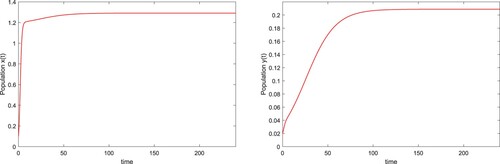
Figure 3. The solutions of system (Equation3(3)
(3) ) with T=3 and
for different initial values. Here we take initial values (0.1, 0.01, 1), (0.08, 0.015, 1), (0.4, 0.08, 0) and (0.8, 0.15, 0).
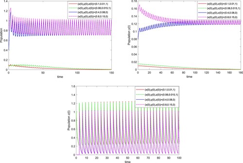
Table 1. Parameter values of the in the laboratory.
However, when we take T=0.5 and , then
and
, from Theorem 3.2, we can get that the periodic solution
is globally asymptotically stable. It means that whatever the initial value is, the wild
population goes to extinction for T=0.5 and
, see Figure . If we take T=6 and
, according to Theorem 3.4, we have
, and the wild
population is strongly persistent in the mean as shown in Figure . From Figures –, we can also see that increasing the release amount β of male
infected with wStri or decreasing the release period T are beneficial to suppress the density of wild
population.
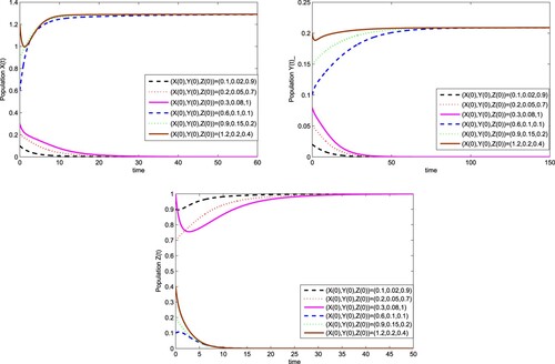
4.2. Long-time behaviours of population replacement model
We first take and T=6, by calculating, we obtain
and
, there exists a locally asymptotically stable wild
eradication periodic solution for system (Equation6
(6)
(6) ) where the wild
population goes to extinction. Furthermore, by selecting appropriate initial values, the numerical simulations show that system (Equation6
(6)
(6) ) also exists a locally asymptotically stable positive periodic solution (see Figure ).
In addition, we consider a special case of system (Equation6(6)
(6) ) that
and
. We obtain
and
by Theorem 3.5, and the equilibrium infected with wStri (0,0,1) is locally asymptotically stable as shown in Figure . It can be seen that we only need to release the
infected with wStri once to the field, and it is possible to complete the replacement of wild
populations.
Figure 4. The solutions of system (Equation3(3)
(3) ) with T=0.5 and
for different initial values. Here we take initial values (0.6, 0.1, 1), (0.8, 0.15, 0.2), (1, 0.2, 0), (1.4, 0.4, 0) and (1.6, 0.5, 0.5).
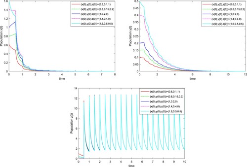
Figure 5. The solution of system (Equation3(3)
(3) ) with T=6,
and the initial value (0.1, 0.05, 1).
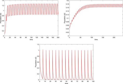
Figure 6. The solutions of system (Equation6(6)
(6) ) with T=6 and
for different initial values. Here we take initial values (0.1,0.02,0.9), (0.2, 0.05, 0.7), (0.3, 0.08, 1), (0.6, 0.1, 0.1), (0.9, 0.15, 0.2) and (1.2, 0.2, 0.4).
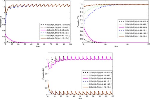
Figure 7. The solutions of system (Equation6(6)
(6) ) with
for different initial values. Here we take initial values (0.1,0.02,0.9), (0.2, 0.05, 0.7), (0.3, 0.08, 1), (0.6, 0.1, 0.1), (0.9, 0.15, 0.2) and (1.2, 0.2, 0.4).
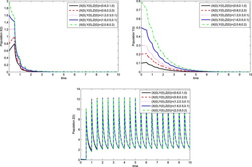
And take and T=0.5, we can get 1−d=−9,
,
and
. It follows from Theorem 3.6 that there exists a globally asymptotically stable wild-
-eradication periodic solution
as shown in Figure . Figure also shows that whatever the initial value is, the wild
population will be replaced by the
infected with wStri when
and T=0.5.
Figure 8. The solutions of system (Equation6(6)
(6) ) with T=0.5 and
for different initial values. Here we take initial values (0.6,0.1,0), (0.8, 0.2, 0), (1.2, 0.3, 0.1), (1.6, 0.5, 0.1) and (2, 0.8, 0.2).
4.3. Control of the wild within a short time
In the first two sub-sections, we fixed parameters ρ, θ, ,
,
and
, and then showed the long-time behaviours of population suppression model and population replacement model by changing parameters β and T. However, it is very important to control the wild
population to a low level in a short time in the actual paddy field management. In this subsection, we will study the effects of release amount β and release period T on the control efficiency of wild
population within a short time under different release strategies. Therefore, we define a concept of control degree as the ratio of the amount of wild
population suppressed or replaced with a finite time to the initial wild
amount [Citation29], denoted by e, and the calculation formula is shown by
where
is the amount of wild
population at time t, and
denotes the initial amount of wild
population. We assume that
,
,
and
.
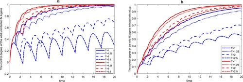
We first consider the effect of the release period T on the control efficiency of wild in a finite time
. Fix parameters
,
,
,
,
and vary T. We take T=1, 1.25, 2 and 2.5, respectively, Both system (Equation3
(3)
(3) ) and system (Equation6
(6)
(6) ) have stable wild-
-eradication boundary periodic solution. From Figure , we can see that the control efficiency of wild
decreases as T increases. For system (Equation3
(3)
(3) ), Figure shows that when
, the control efficiency of the wild
reaches more than
within time
, and when T=2.5, the control efficiency of the uninfected wild
and the wild
infected with wLug within time
is only
and
, respectively. However, the control efficiency of the wild
within time
is more than
for system (Equation6
(6)
(6) ).
Figure 9. The control degree of the wild within a finite time for different release periods. The first four lines of the legend represent the control efficiency of wild
in system (Equation3
(3)
(3) ), and the last four lines of the legend represent the control efficiency of wild
in system (Equation6
(6)
(6) ). (a) The control degree of the uninfected wild
. (b) The control degree of the wild
infected with wLug.
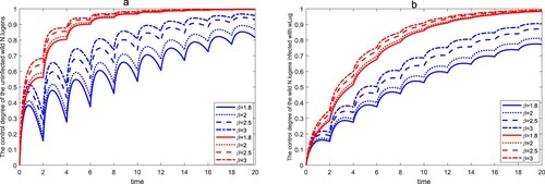
And then, we fix parameters ,
,
,
, T=2 and vary β. Let
and 3, there is also a stable wild-
-eradication boundary periodic solution for both system. Figure shows that the control efficiency of wild
increases as β increases. If we adopt a population suppression strategy, the control efficiency of uninfected wild
within time
is more than
when
, and the control efficiency of wild
infected with wLug within time
is more than
when
. However, when we adopt the population replacement strategy, the control efficiency of wild
within time
is more than
when
.
Figure 10. The control degree of the wild within a finite time for different release amounts. The first four lines of the legend represent the control efficiency of wild
in system (Equation3
(3)
(3) ), and the last four lines of the legend represent the control efficiency of wild
in system (Equation6
(6)
(6) ). (a) The control degree of the uninfected wild
. (b) The control degree of the wild
infected with wLug.
In addition, we consider an ecosystem in which the population of infected with wLug is absent, fix
,
,
,
, and the values of other parameters are the same as those in Figures and , then the time series of the control degree of this wild
population under different release strategies are shown in Figure . It can be seen from Figure that no matter which strategy is adopted, the wild
population will be controlled to more than
in
time. Comparing the results in Figures –, the wild
infected with wLug can reduce the control efficiency of uninfected wild
.
Figure 11. The control degree of the wild within a finite time. The first four lines of the legend represent the control efficiency of wild
in system (Equation19
(19)
(19) ), and the last four lines of the legend represent the control efficiency of wild
in system (Equation23
(23)
(23) ). (a) The effect of β on control degree of the wild
. (b) The effect of T on control degree of the wild
.
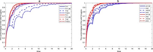
From Figures –, it is easy to see that under the same release amount and release cycle, the efficiency of population replacement strategy in controlling wild within a finite time is significantly higher than that of population suppression strategy. Furthermore, these results also suggest that increasing the release amount β or decreasing the release period T are beneficial for controlling the wild
.
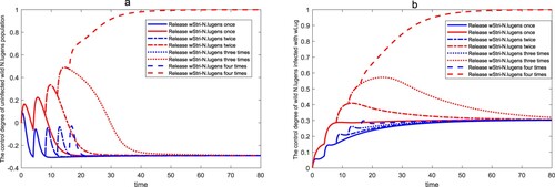
Finally, we will simulate the change of control degree of wild population under a finite release number of times. Fixed parameters
,
,
,
,
, T=4,
,
and
. Based on these parameters, we discuss the situation that the number of release times of
infected with wStri is 1, 2, 3 and 4 respectively, as shown in Figure Equation12
(12)
(12) . It can be seen from Figure Equation12
(12)
(12) that for the population replacement strategy, when the release number of times of
infected with wStri exceeds 3, the wild
population will be controlled. However, for population suppression strategy, it is impossible to achieve complete control of wild
through limited release times. This indicates that the cost of population replacement strategy in controlling wild population will be less than that of population suppression strategy.
In Section 3, we obtained the conditions for the stability of the wild- -eradication periodic solution and verified them numerically in Subsections 4.1–4.2 (see Figures – and –). This also shows that both release strategies are able to control wild
populations. In this paper, both release strategies assume that the
infected with wStri is released in periodic pulses, so the important parameters for control measures are the pulse release amount β and pulse release period T of the
infected with wStri. For population suppression strategy, if the values of the release period T and the release amount β satisfy the conditions of Theorem 3.2, the wild
will become extinct. If the values of β and T satisfy the conditions of Theorem 3.1 but not the conditions of Theorem 3.2, the eradication of wild
depends on the initial values. For population replacement strategy, if the values of T and β satisfy the conditions of Theorem 3.6, the wild
will be replaced. Since the complexity of the expressions for
and
, we cannot directly compare the two strategies theoretically, but we have employed numerical simulations to compare the two strategies in Subsection 4.3, and the population replacement strategy can control wild
faster than the population suppression strategy for the same release period T and the same amount of release β (see Figures –). Moreover, the population replacement strategy can achieve the replacement of the wild
population with a finite number of releases (see Figure ). Of course, the above scenario occurs mainly because there is perfect maternal transmission of female
infected with wStri. However, if the rice population density is added to models (Equation1
(1)
(1) ) and (Equation4
(4)
(4) ), both models will become more complex, which will be one of our next major works. Furthermore, we provided the conditions for the persistence in the mean of wild
in Section 3, but Figure shows the existence of a positive periodic solution for model (Equation3
(3)
(3) ). Unfortunately, we have not found a good mathematical method to solve this problem due to the nonlinearity of the equations, which is also the direction of our future research.
Figure 12. Control of the wild under a finite release number of times. The second, fourth, sixth, and eighth lines of the legend represent the control degree curve of wild
by using population replacement strategy, and the first, third, fifth, and seventh lines of the legend represent the control degree curve of wild
by using population suppression strategy. (a) The control degree of the uninfected wild
. (b) The control degree of the wild
infected with wLug.
5. Conclusions
Gong et al. [Citation6] successfully developed a stable artificial Wolbachia infection of by introducing the Wolbachia strain wStri from
host into
. The use of
infected with wStri to control wild
will be one of the important ways in the future. It is therefore of great interest to study how the release of
infected with wStri. In this paper, we established two models with periodic impulsive release: the population suppression model (Equation3
(3)
(3) ) and the population replacement model (Equation6
(6)
(6) ). Applying Floquet theory and the comparison theorem of impulsive differential equations, we obtained the conditions for the stability of the wild-
-eradication periodic solution of both models (see Figures – and –). Meanwhile, sufficient conditions for the persistence in the mean of wild uninfected
and the extinction of
infected with wLug were obtained, and the conditions for the persistence in the mean of wild uninfected
and
infected with wLug were also given. Numerical simulations were performed to verify our theoretical results. Finally, we compared the control effect of two periodic pulse release strategies on wild
. The population replacement strategy is obviously much better than the population suppression strategy.
Disclosure statement
No potential conflict of interest was reported by the author(s).
Additional information
Funding
References
- S Savary, F Horgan, L Willocquet, et al. A review of principles for sustainable pest management in rice. Crop Prot. 2012;32:54–63. doi:10.1016/j.cropro.2011.10.012
- HJ Huang, YY Bao, SH Lao, et al. Rice ragged stunt virus-induced apoptosis affects virus transmission from its insect vector, the brown planthopper to the rice plant. Sci Rep. 2015;5(1):1–14.
- Z Liu, Z Han, Y Wang. Selection for imidacloprid resistance in Nilaparvata lugens: cross-resistance patterns and possible mechanisms. Pest Manag Sci. 2003;59(12):1355–1359. doi:10.1002/ps.v59:12
- AA Hoffmann, BL Montgomery, J Popovici, et al. Successful establishment of Wolbachia in Aedes populations to suppress dengue transmission. Nature. 2011;476(7361):454–457. doi: 10.1038/nature10356
- X Zheng, D Zhang, Y Li, et al. Incompatible and sterile insect techniques combined eliminate mosquitoes. Nature. 2019;572(7767):56–61. doi:10.1038/s41586-019-1407-9
- JT Gong, Y Li, TP Li, et al. Stable introduction of plant-virus-inhibiting wolbachia into planthoppers for rice protection. Curr Biol. 2020;30(24):4837–4845.e5. doi:10.1016/j.cub.2020.09.033
- H Zhang, KJ Zhang, XY Hong. Population dynamics of noncytoplasmic incompatibility-inducing Wolbachia in Nilaparvata lugens and its effects on host adult life span and female fitness. Environ Entomol. 2010;39(6):1801–1809. doi:10.1603/EN10051
- JF Ju, XL Bing, DS Zhao, et al. Wolbachia supplement biotin and riboflavin to enhance reproduction in planthoppers. ISME J. 2020;14(3):676–687. doi:10.1038/s41396-019-0559-9
- H Noda, Y Koizumi, Q Zhang, et al. Infection density of Wolbachia and incompatibility level in two planthopper species, Laodelphax striatellus and Sogatella furcifera. Insect Biochem Molec. 2001;31(6-7):727–737. doi:10.1016/S0965-1748(00)00180-6
- Z Liu, T Zhou. Wolbachia spreading dynamics in Nilaparvata lugens with two strains. Nonlinear Anal RWA. 2021;62:103361. doi:10.1016/j.nonrwa.2021.103361
- L Cai, S Ai, J Li. Dynamics of mosquitoes populations with different strategies for releasing sterile mosquitoes. SIAM J Appl Math. 2014;74(6):1786–1809. doi: 10.1137/13094102X
- L Cai, S Ai, G Fan. Dynamics of delayed mosquitoes populations models with two different strategies of releasing sterile mosquitoes. Math Biosci Eng. 2018;15(5):1181–1202. doi: 10.3934/mbe.2018054
- J Li. New revised simple models for interactive wild and sterile mosquito populations and their dynamics. J Biol Dynam. 2016;2016:1–18.
- KR Fister, ML Mccarthy, SF Oppenheimer, et al. Optimal control of insects through sterile insect release and habitat modification. Math Biosci. 244(2):201–212. doi:10.1016/j.mbs.2013.05.008
- J Li, ZL Yuan. Modelling releases of sterile mosquitoes with different strategies. J Biol Dynam. 2013;9(1):1–14. doi:10.1080/17513758.2014.977971
- M Huang, X Song, J Li. Modelling and analysis of impulsive releases of sterile mosquitoes. J Biol Dynam. 2017;11(1):147–171. doi:10.1080/17513758.2016.1254286
- J Yu, J Li. Global asymptotic stability in an interactive wild and sterile mosquito model. J Differ Equations. 2020;269(7):6193–6215. doi:10.1016/j.jde.2020.04.036
- B Zheng, J Yu, J Li. Modeling and analysis of the implementation of the Wolbachia incompatible and sterile insect technique for mosquito population suppression. SIAM J Appl Math. 2021;81(2):718–740. doi:10.1137/20M1368367
- J Li, S Ai. Impulsive releases of sterile mosquitoes and interactive dynamics with time delay. J Biol Dynam. 2020;14(1):289–307. doi:10.1080/17513758.2020.1748239
- Z Zhu, B Zheng, Y Shi, et al. Stability and periodicity in a mosquito population suppression model composed of two sub-models. Nonlinear Dynam. 2022;107(1):1383–1395. doi:10.1007/s11071-021-07063-1
- L Hu, M Huang, M Tang, et al. Wolbachia spread dynamics in multi-regimes of environmental conditions. J Theor Biol. 2019;462:247–258. doi:10.1016/j.jtbi.2018.11.009
- L Hu, M Huang, M Tang, et al. Wolbachia spread dynamics in stochastic environments. Theor Popul Biol. 2015;106:32–44. doi:10.1016/j.tpb.2015.09.003
- R Taghikhani, O Sharomi, AB Gumel. Dynamics of a two-sex model for the population ecology of dengue mosquitoes in the presence of Wolbachia. Math Biosci. 2020;328:108426. doi:10.1016/j.mbs.2020.108426
- Z Qu, L Xue, JM Hyman. Modeling the transmission of Wolbachia in mosquitoes for controlling mosquito-borne diseases. SIAM J Appl Math. 2018;78(2):826–852. doi:10.1137/17M1130800
- Z Liu, T Chen, T Zhou. Analysis of impulse release of Wolbachia to control Nilaparvata lugens. Commun Nonlinear Sci. 2023;116:106842. doi:10.1016/j.cnsns.2022.106842
- HJ Barclay. Pest population stability under sterile releases. Res Popul Ecol. 1982;24(2):405–416. doi:10.1007/BF02515585
- J Yu, B Zheng. Modeling Wolbachia infection in mosquito population via discrete dynamical models. J Differ Equ Appl. 2019;25(11):1549–1567. doi:10.1080/10236198.2019.1669578
- V Lakshmikantham, PS Simeonov. Theory of impulsive differential equations. Singapore: World Scientific; 1989.
- J Yu. Modeling mosquito population suppression based on delay differential equations. SIAM J Appl Math. 2018;78(6):3168–3187. doi:10.1137/18M1204917