
 ?Mathematical formulae have been encoded as MathML and are displayed in this HTML version using MathJax in order to improve their display. Uncheck the box to turn MathJax off. This feature requires Javascript. Click on a formula to zoom.
ABSTRACT
HIV continues to be a major global health issue, having claimed millions of lives in the last few decades. While several empirical studies support the fact that proper nutrition is useful in the fight against HIV, very few studies have focused on developing and using mathematical modelling approaches to assess the association between HIV, human immune response to the disease, and nutrition. We develop a within-host model for HIV that captures the dynamic interactions between HIV, the immune system and nutrition. We find that increased viral activity leads to increased serum protein levels. We also show that the viral production rate is positively correlated with HIV viral loads, as is the enhancement rate of protein by virus. Although our numerical simulations indicate a direct correlation between dietary protein intake and serum protein levels in HIV-infected individuals, further modelling and clinical studies are necessary to gain comprehensive understanding of the relationship.
MATHEMATICS SUBJECT CLASSIFICATION:
1. Introduction
Human Immunodeficiency Virus (HIV) is a virus that attacks cells of the human immune system (i.e. cells that help the human body to fight against various infections), making a person more vulnerable to other infections. HIV, which causes acquired immune deficiency syndrome (AIDS), has been a major public health challenge since its first reported case in 1981 [Citation1]. In 2021, approximately 36.7 (1.7) million adults (children) across the world were living with HIV and about 680,000 HIV/AIDS-related deaths were reported [Citation2,Citation3]. Overall, HIV/AIDS has killed approximately 40.1 million humans globally from the time it was first identified (i.e. from 1981) to 2021 [Citation2].
Dynamic interactions between HIV and the human immune system are complex. These interactions have been studied extensively through rigorous mathematical modelling approaches. Most of the research papers on the subject have focused on data- or biologically-driven mathematical models [Citation4,Citation5], while some have been statistical [Citation6,Citation7] or focused on the epidemiology of HIV [Citation8]. A review paper by Jessica M. Conway and Ruy M. Ribeiro summarizes most of the work on the immunology of HIV and offers a comprehensive basis for current work on the topic [Citation9]. Additional sources of information on viral dynamics and immune response to HIV can be found in [Citation10,Citation11].
The fundamental principle behind most of these models is simple: when viral particles meet susceptible cells, they infect the susceptible cells. Some of these infected cells are killed by immune cells, while the other infected cells produce more viruses, leading to a self-sustaining cycle that generates additional infected cells. Although replication of the virus can be modelled with one density-dependent logistic growth equation [Citation11], more elaborate, yet simple models, that are able to capture more biological aspects of the virus require more variables (see, for example, [Citation10,Citation12,Citation13]). These simple mathematical frameworks account for the dynamics of susceptible and infected cells, as well as the free virus, and have been useful in understanding certain aspects of the disease even though they do not capture full biological details of the dynamic interplay between HIV and the immune system. For example, some models in [Citation10,Citation12,Citation13] account for preferential attacks against activated T cells. The simplest models describing interactions between HIV and the immune system, particularly CD8 T cells incorporate an additional compartment for CD8 T cells [Citation12,Citation14]. In addition to these simple models, more complex models have been developed and used to answer more subtle and biologically significant questions on HIV and the human immune system. These models have broad theoretical and practical applications, ranging from CD8 T cell induced pathology [Citation15,Citation16] through modelling of CD8 T cell escape (i.e. the process by which HIV escape recognition by immune effector cells) [Citation17–19] and HIV latency [Citation20–22]. Unfortunately, none of these mathematical models focus on interactions between nutrition, HIV and the human immune system.
Dynamic interplay between nutrition, HIV and the human immune system have been reported. Specifically, HIV weakens the human immune system thereby reducing the ability of the human immune system to fight against diseases significantly [Citation23,Citation24]. On the other hand, the human immune system requires a good nutritional balance to fight such diseases. The formation of immune cells requires various micro and macro nutrients [Citation25–28]. In the absence of proper nutrition, this immune cell formation process can be weakened, rendering a person who is infected with HIV more vulnerable to other opportunistic infections. Although, several studies have focused on the relationship between malnutrition and HIV [Citation29–33], there are still unanswered questions on the impact of dynamic interactions between HIV, immune response to HIV, and nutrition.
Unlike most infectious diseases in which carbohydrates and fats are broken down to supplement the increased nutritional needs of the immune system, HIV induces a special metabolic effect that initiates a preferential loss of proteins over fats and other macro nutrients [Citation34–39]. In particular, HIV is well known for loss of muscle mass and the ‘wasting syndrome’ (i.e. progressive involuntary weight loss of of baseline body weight in the setting of a chronic infection and/or chronic diarrhea [Citation40]) [Citation41,Citation42]. In addition, studies have found some abnormalities in serum protein levels of HIV infected individuals. Serum protein consists of approximately
albumin, which is considered to be a major indicator of malnutrition [Citation43], and approximately
globulin. Studies have found higher levels of serum protein and globulin, and lower levels of albumin in HIV infected individuals compared to their uninfected counterparts [Citation44–47]. A summary of some of the results from various studies that examined the total protein, albumin, and globulin levels in individuals with and without HIV infection is presented in Table . Despite these interesting studies, little to no mathematical modelling effort has been invested in accounting for the relationship between nutrition and human immune response to HIV and the implications of this relationship to HIV dynamics.
Table 1. Total protein, albumin, and globulin levels in individuals with and without HIV infection.
Here, we develop a within-host model for the dynamics of HIV that accounts for interactions between HIV, human immune response to HIV, and nutrition. While this coupled HIV-immune response-nutrition model is new, it is based primarily on well-known within-host HIV models that account for human immune response to HIV [Citation12,Citation49,Citation50]. We incorporate nutrition into the model via protein, which is arguably the most important nutrition factor with regards to HIV. For mathematical tractability, we do not account for separate components of serum protein (such as albumin and globulin). The rest of the paper is organized as follows: The coupled HIV-immune response-nutrition model is developed in Section 2. The immunological reproduction number of the model is computed in Section 3 and used to establish the existence and stability of equilibria to the model system, as well as the existence of a backward bifurcation in Section 3. Numerical simulations to assess the impact of important nutritional parameters on the total protein and HIV viral load are presented in Section 4, while a discussion and concluding remarks are presented in Section 5.
2. The within-host model
2.1. Formation of the within-host model
In this section, we develop a within-host mathematical model for the dynamics of HIV, which accounts for the interactions between HIV, the human immune system, and nutrition. This entails introducing nutrition (specifically, protein) to the target-cell limited model developed in [Citation12] and immune control as in [Citation50]. Since, the primary target of HIV is the CD4 T cells [Citation12,Citation51], we consider CD4 T cells as the target cells cells in our model. These target cells are denoted by T. Infected cells are denoted by , while the virus is denoted by V. Since CD8 T cells constitute the dominant defense mechanism against HIV [Citation12], the cellular immune response is assumed to be dominated by CD8 T cells, which are denoted by Z in our model. Protein is denoted by η. Schematics of the model are depicted in Figure .
Figure 1. Schematic diagram of the within-host model. CD4 T cells are denoted by T, infected cells are denoted by , the virus is denoted by V , CD8 T cells are denoted by Z and nutrition (protein) is denoted by η.
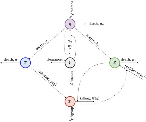
The effect of malnutrition on the immune system is well-documented [Citation29,Citation30]. In particular, studies have shown that malnutrition leads to a decrease in the total number of lymphocytes and CD4 T lymphocytes, while CD8 T lymphocytes are relatively maintained [Citation29,Citation30,Citation52]. Taking this into account, we model the production of target (i.e. CD4 T) cells and the production of immune (i.e. CD8 T) cells as functions of protein, η. Specifically, target (immune) cells are produced at rate r (). Following the target cell limited model in [Citation12], we assume that infected cells (
) are produced at rate
, where V is the population density of the free virus and
–a function of protein is given by
. Here,
is the rate at which target cells are infected per free virus per day and A is a non-negative constant. Observe that the ρ is a decreasing function of η. Target cells die at per capita rate d per day, and the loss of infected cells due to viral cytopathicity is at per capita rate, δ per day. The immune-mediated cytotoxic effect on infected cells by CD8 T cells is modelled with the term
, where
is the rate at which infected cells are killed by activated CD8 T cells,
is the killing rate of infected cells per CD8 T cell per day and Ψ is the half-saturation constant. It should be noted that Ψ allows the killing rate of infected cells to be independent of nutrition, while A in
allows us to remove the dependence of the infectivity rate of target cells on nutrition. Virions (V) are produced from infected cells (
) at rate of p and cleared naturally at per capita rate c. The clearance of virus by immunoglobulins is modelled by the term
, where
is the virus clearance rate by immunoglobulins per gram of protein per day. In the presence of higher protein levels, the immunoglobulin levels are also higher and in this case, we assume that the virus is cleared at a faster rate. Following [Citation12], the activation of CD8 T cells is modelled by the term
that is dependent on the density of infected cells, where b is the antigen activation rate per infected cell per day. The per capita death rate of CD8 T cells
per day. The generation rate of protein is
grams per day, the per capita clearance rate of protein is
per day, while virus-driven increase in total protein levels is modelled by the term
, where
is the enhancement rate of protein per virus per day. It is worth noting that the positive term
coincides with the observed high levels of serum protein in HIV infected individuals. While this term may seem somewhat counter-intuitive, it aligns with the biological data at hand [Citation44,Citation46–48], previous studies on the subject[Citation52] and our numerical simulations. We hypothesize that an increased presence of viral activity in body due to HIV infection leads to an increased antibodies (immunoglobulins) and this in turn leads to higher levels of globulin and serum protein. The cause and effect of this significant phenomena is further discussed in Section 5 where all our results are compared with already existing biological data. Brief descriptions of the model parameters and their units, as well as numerical values are presented in Table .
Using the schematics in Figure together with the variable and parameter descriptions above, we obtain the following coupled HIV-Immune response-nutrition model: (1)
(1)
Table 2. Brief descriptions of the parameters of the within-host model together with the numerical values and units of the parameters and initial conditions.
2.2. Existence, uniqueness, positiveness and boundedness of solutions
The existence of a unique, positive solution locally in time can easily be verified for the system given by (Equation1(1)
(1) ). Let
be defined by
, where
, and
denote the five differential equations in the system. Since F and
are continuous on
, F is locally Lipschitz. Now, the existence of a unique, positive solution defined on some interval
with
follows by Theorem A.4 in [Citation53].
The boundedness of solutions of the system given by (Equation1(1)
(1) ) cannot be established without further imposing conditions on model parameters. In fact, in Appendix 1, we establish the boundedness of solutions under certain assumptions on parameter values.
2.3. Limitations of the model
Model (Equation1(1)
(1) ) is based on some simplifying assumptions, which might limit its applicability. However, relaxing some of these assumptions will render the model more complex and mathematically intractable. For example, a logistic-like growth function can be used for the growth of CD4 T cells to account for the data measuring the number of dividing helper cells in HIV infected individuals with different CD4 T cell counts [Citation12]. But this will make the within-host model more complicated since we must also take the nutritional aspects into consideration. Also, the immune control component of the model, given by the fourth equation of (Equation1
(1)
(1) ), can be made more realistic by using an activation function that saturates [Citation12,Citation50], e.g.
(2)
(2) Here,
is the maximal rate of CD8 T activation. Furthermore, we can improve on the way cellular immunity is modelled. For example, immune impairment due to high viral loads, and hence high infected cell densities, can be taken can be modelled through another saturation function [Citation50], which will lead to the following modified version of the fourth equation of (Equation1
(1)
(1) ):
(3)
(3) Additionally, considering abnormalities related to albumin and globulin concentrations in HIV-infected individuals, albumin and globulin can be modelled separately, instead of the total protein (see, for example, [Citation52]).
The four linear functions of η, namely, and
were assumed to be linear for the sake of mathematical and analytical simplicity. These four functions, however, are unbounded and increasing to ∞ as
. Due to nutrition's limited role in fighting the virus, it would be more realistic to use saturated functions in place of these linear functions.
3. Analytical results
3.1. The infection-free equilibrium 
Equilibria are important in determining the long-term behaviour of solutions to autonomous systems of differential equations that cannot be solved analytically [Citation54]. To identify the equilibria of the model (Equation1(1)
(1) ), we set the left-hand sides of the system to zero and solve the resulting system of algebraic equations for five state variables
, and
(where the ‘*’ denotes ‘the equilibrium value of ’) simultaneously. Specifically, any equilibrium point
, of the model (Equation1
(1)
(1) ) must satisfy the following system of equations:
(4)
(4) Solving for
, and
in terms of
from the first, third, fourth, and fifth equations of system (Equation4
(4)
(4) ) leads to
(5)
(5)
(6)
(6)
(7)
(7)
(8)
(8) It should be noted that for defined and non-negative equilibria,
. From the second equation of the system (Equation4
(4)
(4) ), i.e.
(9)
(9) and (Equation5
(5)
(5) )–(Equation9
(9)
(9) ), it is clear that
is a solution of (Equation4
(4)
(4) ). This is the infection-free equilibrium value of
, which we will denote by
. To obtain the infection-free equilibrium values of the other state variables (i.e.
, and
) denoted by
, and
, respectively, we substitute
in Equations (Equation5
(5)
(5) )–(Equation9
(9)
(9) ). This gives
(10)
(10)
3.2. Immunological reproduction number ()
The immunological reproduction number, , represents the number of secondary virus particles that one viral particle will produce in an entirely susceptible target cell population through out the period within which the viral particle is capable of producing secondary virus particles. In this Section, we compute the reproduction number of the model (Equation1
(1)
(1) ) using two approaches–the next generation operator approach proposed by van den Driessche and Watmough [Citation55] and an intuitive approach with a direct biological interpretation.
3.2.1. Reproduction number through the next generation operator approach
In this subsection, we use the next generation operator technique proposed by van den Driessche and Watmough [Citation55] to calculate the immunological reproduction number of the within-host model given by system (Equation1(1)
(1) ). Following this method and using the same notation as in [Citation55], we define the matrices of new infections (F) and transitions V as follows:
where
is the vector of new infections,
is the vector of new transition terms,
,
, and
, with
is the unique unique equilibrium of the infection-free system
. The next-generation matrix is then defined by
The reproduction number of the model system (Equation1
(1)
(1) ) is then defined to be the spectral radius of the next-generation matrix,
. The eigenvalues of the
matrix (
) are given by the characteristic equation:
, which simplifies to
Thus, the reproduction number from the next-generation operator approach is
(11)
(11) Since
and
, where
, and since
, the expression for the reproduction number in (Equation11
(11)
(11) )) can be simplified to
(12)
(12)
3.2.2. Reproduction number through the intuitive approach
While the immunological reproduction number can be calculated using the next generation operator method, the biological interpretation of this important threshold might not be obvious from the final expression (especially due to the square-root in this expression). In this section, we derive the reproduction number through an intuitive approach in which terms and expressions and associated with meaningful biological interpretations.
Each infected cell produces virus at rate p. Also, infected cells die at rate δ due to viral cytopathogenic effects, or at rate , where
and
(given in (Equation10
(10)
(10) )) are the infection-free equilibrium values of CD8 T cells and protein, respectively, due to immune-mediated cytotoxic effects. Because infected cells are cleared at a total rate of
, they live, on average, for
days. Therefore, on average, each infected cell produces
virions during its lifetime. On the other hand, Now, virions are cleared naturally at a per capita rate c, or by immunoglobulins at rate of
. Thus, virions are cleared at a total rate of
. Hence, on average, each virion lives for
days. During this time, each virion infects
susceptible cells on average. Thus, the total number of cells infected by
virions released from one infected cell is given by
. Thus,
3.2.3. Comparing the reproduction numbers from the next generation operator and intuitive approaches
When the reproduction number is greater than 1, the reproduction number obtained using the intuitive approach produces a higher value compared to the reproduction number obtained using next generation operator approach
. On the other hand, if the reproduction number is less than 1, the relationship between the two reproduction numbers is reversed. Specifically, the reproduction number from the intuitive approach is the square of that from the next generation operator approach, i.e.
However, the intuitive derivation process is more informative as it provides meaningful biological interpretations for the two non-zero entries (
and
) in the next generation operator approach. Irrespective of the difference, the epidemiological/immunological implications of the reproduction number that the disease can be cleared when
, or can persist when
, remains the same since
and
.
3.3. Stability of the infection-free equilibrium
Local stability of the infection-free equilibrium () of the model (Equation1
(1)
(1) ) will be establish by considering the signs of the eigenvalues of the Jacobian of the model system computed at
. This Jacobian is given by
From the Jacobian (
), it is clear that three of the eigenvalues are
, and
and that the remaining two eigenvalues are eigenvalues can be determined from the
sub-matrix
Since the first three eigenvalues are negative, all we need to do to establish the stability of the infection-free equilibrium is to determine the signs of the two remaining eigenvalues. To this effect, we use Theorem 3.2 from [Citation54], which states that a
matrix is stable if the trace of the matrix is negative and the determinant is positive. Hence, we need to determine whether
and
. The trace of
is given by
, which is negative, while the determinant of
is given by
, if
. Hence, we have the following standard result:
Theorem 3.1
If , then the infection-free equilibrium (
) is locally asymptotically stable. If
,
is unstable.
3.4. Existence of infection equilibria and backward bifurcation
In this Section, we show that the model system (Equation4(4)
(4) ) has a unique infection equilibrium when the reproduction number is greater than unity and that there is a parameter regime within which the model exhibits a backward bifurcation when the reproduction number is less than unity. The existence of a backward bifurcation implies that measures aimed at clearing the virus must be sustained even when the reproduction number is slightly less than one until the reproduction number falls below a smaller threshold value.
3.4.1. Existence of unique infection equilibrium
All equilibria of the model system (Equation4(4)
(4) ) must be non-negative. Hence, as indicated in Section 3.1, we must have
. From (Equation8
(8)
(8) ),
(13)
(13) where
and
can be determined from (Equation9
(9)
(9) ). For
to be positive, the denominator of the right-hand side must be positive. That is, we must have
(14)
(14)
The left-hand side () of the inequality (Equation14
(14)
(14) ) is a straight line that goes through the origin, while the right-hand side (
) is a parabola with roots
and
Figure . The parabola opens up (since the coefficient of
is positive) and meets the straight line
at two distinct points (
and
), with
. Then
and hence
. Since this satisfies our requirement for positive infection equilibrium values,
.
Next, considering (Equation9(9)
(9) ) with
and
given by Equations (Equation5
(5)
(5) )–(Equation8
(8)
(8) ), we have
(15)
(15) Let
and
. Here,
is decreasing on
, while
is increasing on
(see Appendix 1). Thus, if a solution exists, it must be unique. We prove the existence of a solution as follows. Since
, we set V =0 in
and
to obtain
Now,
(16)
(16) That is,
. Similarly, we set
to obtain
Thus,
. Since
is decreasing on
,
is increasing on
,
and
,
and
meet at one point, say,
. When
, Equation (Equation15
(15)
(15) ) has a unique root on
. Hence, Equation (Equation15
(15)
(15) ) has a unique positive solution
. Consequently, the model system (Equation4
(4)
(4) ) has a unique infection equilibrium,
, with
and
given by Equations (Equation5
(5)
(5) )–(Equation8
(8)
(8) ) and
given by (Equation9
(9)
(9) ). This proves the following theorem:
Figure 2. Graphical representation of inequality (Equation14(14)
(14) ).
![Figure 2. Graphical representation of inequality (Equation14(14) pμZ(μη−γηV∗)>bV∗[c(μη−γηV∗)+λημV]⇔bλημVV∗<(μη−γηV∗)(pμZ−bcV∗).(14) ).](/cms/asset/50d3aa89-af00-4402-b3d2-769b8a826c3c/tjbd_a_2287087_f0002_oc.jpg)
Theorem 3.2
There exists a unique infection equilibrium of the system (Equation1
(1)
(1) ) when
.
It should be noted that (Equation8(8)
(8) ) shows that the amount of protein at equilibrium (
) is an increasing function of the equilibrium viral load (
), which is consistent with results from other studies that have found higher total protein concentrations in people with HIV compared to people without HIV [Citation44,Citation47].
3.4.2. Backward bifurcation
In this subsection, we explore the possibility of backward bifurcation for the within-host model given by (Equation1(1)
(1) ). Although we will not discuss the theoretical background and biological implications of the phenomenon, we will derive a necessary and sufficient condition for its existence.
We apply the Center Manifold Method proposed in [Citation56,Citation57] to establish the existence of a backward bifurcation in the system (Equation1(1)
(1) ). The first step involves choosing a bifurcation parameter (ϕ) such that
is an increasing function of ϕ. In this case, we use p as the bifurcation parameter. It can be verified that
is an increasing function of p. Let
be the value of p for which
. That is,
(17)
(17) When
, the Jacobian of the model (Equation1
(1)
(1) ) evaluated at the infection-free equilibrium (
) has a simple eigenvalue of zero and all other eigenvalues are negative. Specifically, when
, the eigenvalues of
are
, and
. The right eigenvector for the simple eigenvalue zero is given by
, where
Observe that,
may not be non-negative. However the method can still be applied since
corresponds to a positive entry in the infection-free equilibrium [Citation57]. Now, if
is the left eigenvector for the simple eigenvalue zero, then
The left eigenvector has all zero components except
and
. Define,
for
by
(18)
(18) First, we calculate
, where
,
,
,
and
. Plugging in
,
and
, for m=2, and
, for
the sum b becomes
(19)
(19) which is clearly positive. Next, we calculate
. The non-zero partial derivatives of
and
at
are given below:
(20)
(20) Since
, the formula for a becomes:
(21)
(21) We substitute (Equation20
(20)
(20) ) in (Equation21
(21)
(21) ) and simplify the above expression to get:
(22)
(22) This leads to the following result:
Theorem 3.3
A backward bifurcation occurs in the model (Equation1(1)
(1) ), if and only if
, where a is given by (Equation22
(22)
(22) ).
Assuming that , the expression for a (i.e. (Equation22
(22)
(22) )) simplifies to
. Furthermore, since all parameters involved in a are positive,
if and only if
. By substituting
, and
in (Equation22
(22)
(22) ), we obtain the condition
. Hence we have the following corrollary:
Corollary 3.4
Let and
. Then the model (Equation1
(1)
(1) ) exhibits a backward bifurcation.
4. Model parameters and numerical simulation results
4.1. Model parameters
Most of the standard parameters of the model (Equation1(1)
(1) ) are available in the literature. However, the nutritional parameters remain unclear and hence unknown. This is due to the lack of within-host models that couple the dynamics of HIV and nutrition. Therefore, we use available data to estimate numerical values for the nutritional parameters.
The normal range for total protein in the human body is 60 to 80 grams per litre of blood [Citation58]. Here, we consider an average value of grams per litre. The amount of blood circulating within a human depends on the human's size and weight. But the average adult has nearly 5 litres of circulating blood [Citation59]. Therefore, an average adult has a total of
grams of protein in their body. Hence, we assume that the equilibrium value of η is
grams of protein.
The estimated lifetime of CD4 T cells is 100 days. Since on average this is the same as , d=0.01 per day [Citation50]. We assume that CD4 T cells are produced at a rate of
cells per μ L of blood per day [Citation50], so that the recruitment rate of CD4 T cells per gram of total protein is
cells per μ L of blood per day per gram of protein. The infection rate of target cells is taken to be
of blood per virion per day [Citation50], so that the infection rate of target cells is
grams of protein μ L of blood per virion per day. The proportionality constant for nutrition, A, is assumed to be 0.1 per gram of protein. Infected cells die at rate
per day, and the strength of CD8 T cell response is
L of blood per CD8 T cell per day [Citation50]. The half-saturation constant for nutrition, Ψ, represents the density at which half of the equilibrium protein intake is reached and is given by
grams of protein. The number of virions produced by an infected CD4 T cell during its lifetime, N, is estimated to be between a few hundred to tens of thousands of virions. Following [Citation50], we take and the average value of N=2000 virions per CD4 cell, so that the virus production rate, p, is given by
virions per CD4 cell per day. The viral clearance rate is c=23 per day [Citation50]. The CD8 T cell production rate is given by
CD8 cells per μL of blood per day [Citation50]. Hence, the recruitment rate of CD8 T cells per gram of total protein is given by
CD8 cells per μL of blood per gram of protein per day. The antigen driven activation rate of CD8 T cells is b=1 per day [Citation50], and the CD8 T cells die at a rate of
per day [Citation50]. The rate of ingestion of total protein,
, is calculated as the average weight of 180 pounds multiplied by the Dietary Reference Intake (DRI) of 0.36 grams of protein per pound per day [Citation60]. This is approximately 65 grams per day.
The rate of clearance of virus particles by immunoglobulins, , is calculated by solving the third equation of Model (Equation1
(1)
(1) ) for
. This gives
. We assume a typical viral load of
virions per μL of blood, and
cells per μL of blood [Citation12]. These estimates, together with p=2000 virions per CD4 cell per day and c=23 per day gives
per gram of protein per day. Similarly, solving the fifth equation of (Equation1
(1)
(1) ) at equilibrium we get
. Assuming that
per day, we get
per day.
Numerical simulations, as well as predictions of the model (Equation1(1)
(1) ) depend on the initial conditions. Hence, we estimate the initial conditions that will be used for the numerical simulations here. A normal CD4 T count is from 500 to
cells per cubic millimeter of blood [Citation61]. That is, in
of peripheral blood, there are 1000 CD4 T cells. Following [Citation62], we fix the density of target cells before infection (i.e.
), at
of the CD4 T cell density in peripheral blood and assume that there are no infected cells initially (i.e.
). Based on [Citation62], we take the initial viral load (
), to be
virions per
of blood to represent the presence of a small number of virions following primary infection. The normal range for an absolute number of all CD8 T cells, which includes both killer and suppressor T cells, is 150 to 1, 000 cells per cubic millimeter of blood [Citation63]. For simplicity, we assume an average of
cells per
of blood. The numerical values of these model parameters and initial conditions are summarized in Table .
4.2. Numerical simulation results
In this section the within-host model given by (Equation1(1)
(1) ) will be simulated using the parameter values presented in Table to assess the impact of some of the important nutritional parameters on the behaviour of protein and viral levels. Primary HIV infection is defined as the first six months after acquiring HIV and is considered to be the most crucial period in terms of disease management [Citation64]. During this period, plasma viremia reaches a peak (usually after 21-28 days) [Citation65]. The intensity and timing of the peak, as well as the equilibrium viral load are important factors that define the trajectory of the disease. Hence, it is important to understand the impact of important model parameters on the viral load, as well as other variables during this period.
4.2.1. Assessing the impact of the viral production rate (p)
The model (Equation1(1)
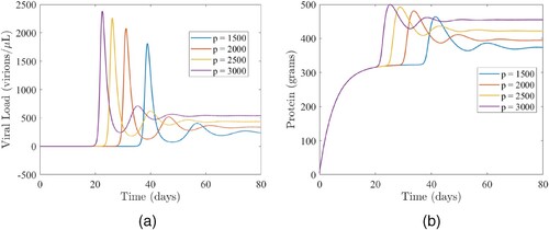
(1) ) is simulated using the parameter values in Table to explore the impact of the viral production rate (p), on the viral load and total protein. Results of the simulations depicted in Figure show that the equilibrium viral load is strongly dependent on the viral production rate Figure (a), which and is consistent with results from previous studies [Citation66]. As expected, increases in the viral production rate will lead to increases in the peak viremia size and total protein, as well as speed up the time for which the viremia and total protein peak. In particular, for the baseline viral production rate of p=2000, the viremia (total protein) peaks on day 31 (34), with a peak size of 2079 virions per μ L and 481 grams of total protein (red curves in Figure ). Reducing the viral production rate from its baseline value of p=2000 to p=1500 (i.e. by
), will lead to a
(
) reduction in peak size of the viral load (total protein) and a 8-day increase in the time that the viremia peaks, as well as a 7-day increase in the time for the total protein to peak (comparing the red and blue curves in Figure ). At equilibrium, a
(
) reduction in the viral load (total protein) is recorded. However, increasing the viral production rate from its baseline value of p=2000 to p=3000 (i.e. by
), will lead to a
(
) increase in the peak size of the viral load (total protein) and a 9-day decrease in the time that the viremia peaks, as well as a 9-day decrease in the time that the total protein peaks (comparing the red and purple curves in Figure ). For this scenario, a
(
) increase in the equilibrium viral load (total protein) is recorded. In summary, there is a positive correlation between the viral production rate (p) and the viral load and serum protein and a negative correlation between the times at which the viral load and total proteins peak.
Figure 3. The impact of the viral production rate (p) on (a) the viral load and (b) total protein. (a) Simulations of the model (Equation1(1)
(1) ) depicting the impact of the viral production rate (p) on the viral load. The other parameters used for the simulations are presented in Table . (b) Simulations of the model (Equation1
(1)
(1) ) depicting the impact of the viral production rate (p) on total protein. The other parameters used for the simulations are presented in Table .
4.2.2. Assessing the impact of the protein intake rate
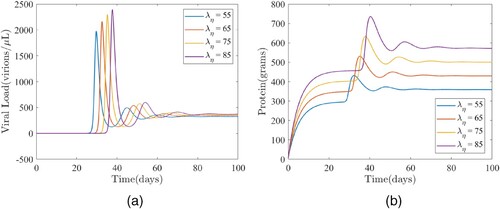
The model (Equation1(1)
(1) ) is simulated using the parameter values in Table to investigate the relationship between the dietary protein intake (
) and the viral load and total protein. The results show that increasing the dietary protein intake will trigger an increase in the viral load and total protein level, as well as the time for the viral load and protein to peak Figure . Specifically, if all parameters are maintained at their baseline values given in Table (including the baseline dietary intake value of
), the viral load (total protein) will attain its first peak on day 33 (35), with a viral peak size of 2164 virions per μL and a total protein peak size of 531 grams (red curves in Figure ). If the baseline value of the protein intake rate is reduced by approximately
(i.e. setting
), a
reduction from the baseline peak size of the viral load will be recorded (comparing the red and blue curves in (a)), while a
reduction from the baseline peak size of total protein will be recorded (comparing the red and blue curves in (b)). For this scenario, a 3-day reduction in the time for both the viral load and total protein to peak will be recorded, while a
(
) reduction in the equilibrium level of the viral load (total protein) will be recorded. On the other hand, an approximate increase of
in the baseline protein intake rate (i.e. setting
) will result in a
increase in the equilibrium viral load and a
increase in the total protein levels (comparing the red and purple curves in ). In summary, for the values of
considered in this study, the viral load (total protein) attains a peak between
and
(
and
) weeks of primary infection.
Figure 4. The impact of the protein intake () on (a) the viral load and (b) total protein. (a) Simulations of the model (Equation1
(1)
(1) ) depicting the impact of the protein intake (
) on the viral load. The other parameters used for the simulations are presented in Table . (b) Simulations of the model (Equation1
(1)
(1) ) depicting the impact of the protein intake (
) on total protein. The other parameters used for the simulations are presented in Table .
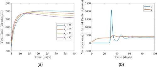
Additional simulations of the model (Equation1(1)
(1) ) were carried out to investigate the factors that contribute to the observed positive correlation between the dietary protein intake and serum protein Figure (a). For this case, we set the virus production rate (p) to 6000 (which is somewhat unrealistic), the strength of CD8 T response (
) to
L per cell per day, vary the protein intake rate from 55 to 85 and maintain the remaining parameters at their baseline values given in Table . As expected, increasing the protein intake rate (
), leads to an increase in the viral load initially Figure (a). However, this changes after the third week of primary infection and after the beginning of the third week, increasing
is associated with a decreasing viral load Figure (a). This implies that there is a negative correlation between the intake rate of total protein and viral load when the strength of the CD8 T response is increased to an extremely high level along with higher viral production rates.
The discussion on the amount of virus present during the primary infection aligns with previous observations: a high level of virus in the bloodstream, which is later controlled by the body's immune system [Citation64]. However, there is one critical observation regarding viral loads and serum protein levels that is unique to this study. Specifically, peak viral loads are almost always quickly followed by peak serum protein levels until equilibrium is attained (see, for example, Figure (b)).
Figure 5. (a) The impact of the protein intake () on the viral load and (b) the dynamics of the viral load (V) and total protein (η). (a) Simulations of the model (Equation1
(1)
(1) ) illustrating the impact of the protein intake rate (
) on viral load. For these simulations,
, and the other parameter values are as given in Table . (b) Simulations of the model (Equation1
(1)
(1) ) illustrating the dynamics of the viral load (V) and total protein (η). Parameter values are as fixed at their baseline values given in Table .
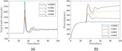
4.2.3. Assessing the impact of the enhancement rate of protein by the virus
In this Section, the model (Equation1(1)
(1) ) is simulated to assess the impact of the enhancement rate of protein by the virus (
) on both the viral load and total protein. It should be noted that there is little to no experimental data or research on
that could be used to evaluate or approximate
. This is simply due to the lack of mathematical modelling with regards to the role of protein in HIV. Therefore, for numerical simulations we use an assumed value of 0.0001 per day for
, the enhancement rate of protein by virus. The results obtained and illustrated in Figure show that the peak viral load (respectively, peak total protein) occur around the same time (on day 33 for the viral load and day 35 for total protein) during primary infection (comparing the primary infection peaks in Figure (a,b), respectively). This suggests that the time at which the peak viremia or protein occurs is independent of
. Furthermore, the simulations show that increasing the enhancement rate of protein by the virus leads to increased equilibrium viral loads and total proteins, although the difference in equilibrium viral load is indiscernible. Interestingly, an increasing enhancement rate of protein by the virus will be associated with decreasing peak viral load. In particular, if the enhancement rate of protein by the virus is increased from its baseline value of
to
, a decrease of
in the peak size of the viral load and a slight increase of
in the equilibrium viral load will be observed (comparing the red and yellow curves in Figure (a)), while an increase of
in the peak total protein levels and an increase of
in the equilibrium protein level will be observed (comparing the red and yellow curves in Figure (b)). Additional increases from the baseline value of the enhancement rate of protein by the virus will lead to more increases in the equilibrium values of both the viral load and total protein (comparing the red curve with the other curves in Figure ).
Figure 6. The impact of the protein intake () on (a) the viral load and (b) total protein. (a) Time series plot of the model (Equation1
(1)
(1) ) showing the effects of the enhancement rate of protein by the virus (
) on the viral load (V). The values of the other parameter used for the simulations are as given in Table . (b) Time series plot of the model (Equation1
(1)
(1) ) showing the effects of the enhancement rate of protein by the virus (
) on the total protein level (η). The values of the other parameter used for the simulations are as given in Table .
5. Discussion
In this study, we developed a within-host mathematical model for the dynamics of HIV, which accounts for interactions between HIV, the human immune system, and nutrition. The model is based on the target cell limited model developed in [Citation12]. The first phase involved introducing immune control in this basic model based on the mathematical frameworks in [Citation12,Citation50]. The main novelty of the model framework involves the introduction of nutrition in the form of protein primarily due to its importance in the context of HIV. The goal of this study is to clear some of the misconception regarding HIV and the role of malnutrition in HIV infection and to shed some light on related unanswered questions.
Rigorous mathematical analysis of the model including existence, uniqueness and positivity of solutions was carried out. The immunological reproduction number was computed (using two different approaches) and used to establish standard results related to the existence and stability of an infection-free equilibrium and the existence of endemic equilibria. In particular, it was shown that a unique infection equilibrium exists when the immunological reproduction number is greater than one and that when the immunological reproduction number is less than one, there is a parameter regime within which a backward bifurcation occurs. Additionally, necessary and sufficient conditions for the existence of this backward bifurcation were derived using the centre manifold theory method.
According to a recent study which focused on the nutritional state of HIV infected adults in the United States, the total protein levels of HIV infected individuals were found to be higher compared to their non-infected counterparts [Citation44]. According to the study, non-infected women have, on average, grams of protein per litre of blood, whereas HIV infected women have
grams per litre, which is almost a
increase compared to non-infected women. Infected men, on average, have
grams of total protein per litre of blood, compared to
grams per litre of non-infected men, which is a
boost in total protein levels compared to non-infected men. According to another study in which serum protein electrophoresis was performed on 70 HIV-positive and 42 HIV-negative controls, the control group, on average, has 75.5 grams of protein per litre of blood, whereas the HIV infected group, on average, has 85.4 grams per litre,
more than the control group [Citation47]. A similar study on serum protein electrophoresis pattern in patients living with HIV in Iran, however, reveals that, unlikely in the United States, a total protein concentrations of HIV infected individuals were lower than that of the control group, i.e. non-infected individuals [Citation46]. The dietary protein intake of individuals involved in the study mentioned above, Thuppal et al. [Citation44], leads us to some interesting hypothesis. According to the study, the daily protein intake of HIV infected women in the United States, on average, is
grams, and this is approximately
higher than the average daily protein intake of non-infected women, which is
grams. While this increase in intake of protein can be labelled as being cautious or vigilant about their diets after diagnosed with HIV, it does not necessarily imply that there is any significant correlation between this increased dietary protein intake and increased serum protein levels. Interestingly, our numerical simulations also suggest that the dietary protein intake is in direct correlation with total protein when other parameters of the model are kept constant. This however may not be an accurate portrayal of the situation.
Firstly, the usual scientific consensus is that an increased protein intake does not cause high levels of protein in blood [Citation67]. Whether or not this is true in case of HIV infected individuals remains to be understood. Secondly, the same study discussed previously, Thuppal et al. [Citation44], reveals that while HIV infected men in the United States have total protein levels that are higher than that of non-infected men, unlike women, HIV infected men do not have an increased dietary protein intake compared to non-infected men. In fact, the daily protein intake of HIV infected men, on average, is
grams and that of non-infected men is
grams. The difference is almost indiscernible. Finally, the results we obtained with respect to the relationship between dietary protein intake and serum protein levels could simply be due to the lack of complexity of the model. The maintenance of blood protein levels in the human body is a complicated process that involves multiple organs (such as lever, kidneys) and mechanisms working hand-in-hand to regulate protein production, removal and homeostasis in the blood. For example, the clearance of albumin alone is a complicated process which is due to
renal activity,
gastrointestinal activity and
catabolic clearances [Citation68]. In our model, the protein ingestion is considered constant and the removal of protein is assumed to be proportional to the amount of protein in blood, which may not accurately explain the situation. Our model, as insightful as it is, may not be able to capture and account for all these subtle biological details. Now, a question that arises naturally is, ‘what other factors, may they be internal or external, would contribute to the observed increment in total protein levels in HIV infected individuals?’. While we still do not possess a full understanding of what factors cause the total protein levels to go up, and more importantly, how these factors contribute to these high levels of blood protein in HIV infected individuals, it is safe to assume that this is caused, or at least catalyzed, by the presence of the virus in the body.
The increased total protein during HIV infection could be explained, at least to a certain extent, by observing the dynamics between HIV, immune system and nutrition. Due to the infection, there is an increased presence of antibodies (immunoglobulins), and this leads to higher levels of globulin, and consequently, to higher total protein levels in blood. This argument is backed by many studies. According to [Citation47], Immunoglobulin G (IgG), the most common antibody, levels in HIV infected individuals are much higher than that of non-infected individuals. The average IgG level in 70 HIV infected individuals is 27.0 grams per litre, a massive higher than an average of 16.0 grams per litre in 42 non-infected individuals (see Table 1). These facts are backed by many other studies [Citation48,Citation69]. In fact, our results suggest that an increased enhancement rate of protein by the virus,
, leads to increased equilibrium protein levels. Furthermore, our numerical simulations suggest a positive correlation between
and equilibrium viral loads. This is to be expected as a higher
value is an indicator of high viral activity in the body.
During the course of our study, numerical simulations were carried out to study the effect of the ingestion rate of protein, , on HIV viral loads. Our results suggest that with an increasing rate of ingestion of protein, the viral loads also increase, although the difference in equilibrium viral loads is almost indiscernible. While this is a somewhat complex issue and there seems to be no clear consensus in the scientific literature, consistent with our results, a study on the impact of high protein intake on viral load and hematological parameters in HIV infected patients suggests that excess dietary protein and L-lysine can increase the risk of high HIV replication, subsequent acceleration of immunosuppression and the disease progression [Citation70].
The relationship between p, the viral production rate, and serum protein levels is interesting, and somewhat expected. A study published on the PNAS (Proceedings of the National Academy of Sciences) on HIV replication found that when HIV is supplemented with human serum in vitro, the HIV replication rates were increased [Citation5]. While the protein content in human serum is about , this could be due to a positive correlation between the viral production rate and serum protein. This hypothesis is further confirmed by our numerical simulations.
In conclusion, the viral production rate is in positive correlation with HIV viral loads, as is the enhancement rate of protein by virus. The effect of dietary protein intake on HIV viral loads and serum protein should further be studied with the aid of clinical studies coupled with mathematical modelling in order to draw more accurate conclusions.
Disclosure statement
No potential conflict of interest was reported by the author(s).
Additional information
Funding
References
- P Lewthwaite, E Wilkins. Natural history of HIV/AIDS. Medicine. 2009;37:333–337. doi: 10.1016/j.mpmed.2009.04.015
- USAIDS. Global HIV & AIDS statistics, Fact sheet (Accessed on March 27, 2023). https://www.unaids.org/en/resources/fact-sheet. Online Version.
- World Health Organization. HIV: global situation and trends. Global Health Observatory (Accessed on March 27, 2023). https://www.who.int/data/gho/data/themes/hiv-aids. Online Version.
- D Burg, L Rong, AU Neumann, et al. Mathematical modeling of viral kinetics under immune control during primary HIV-1 infection. J Theor Biol. 2009;259:751–759. doi: 10.1016/j.jtbi.2009.04.010
- MF Perdomo, W Hosia, A Jejcic, et al. Human serum protein enhances HIV-1 replication and up-regulates the transcription factor AP-1. Proc Natl Acad Sci. 2012;109:17639–17644. doi: 10.1073/pnas.1206893109
- T Zhu, J Zhong, R Hu, et al. Patterns of white matter injury in hiv infection after partial immune reconstitution: a DTI tract-based spatial statistics study. J Neurovirol. 2013;19:10–23. doi: 10.1007/s13365-012-0135-9
- M Ciupe, B Bivort, D Bortz, et al. Estimating kinetic parameters from HIV primary infection data through the eyes of three different mathematical models. Math Biosci. 2006;200:1–27. doi: 10.1016/j.mbs.2005.12.006
- G Maartens, C Celum, SR Lewin. HIV infection: epidemiology, pathogenesis, treatment, and prevention. The Lancet. 2014;384:258–271. doi: 10.1016/S0140-6736(14)60164-1
- JM Conway, RM Ribeiro. Modeling the immune response to HIV infection. Curr Opin Syst Bio. 2018;12:61–69. doi: 10.1016/j.coisb.2018.10.006
- M Nowak, RM May. Virus dynamics: mathematical principles of immunology and virology: mathematical principles of immunology and virology. UK: Oxford University Press; 2000.
- D Wodarz. Killer cell dynamics: mathematical and computational approaches to immunology. New York (NY): Springer; 2007.
- RJ De Boer, AS Perelson. Target cell limited and immune control models of HIV infection: a comparison. J Theor Biol. 1998;190:201–214. doi: 10.1006/jtbi.1997.0548
- RM Anderson, RM May. Infectious diseases of humans: dynamics and control. Oxford (UK): Oxford University Press; 1991.
- MA Nowak, CR Bangham. Population dynamics of immune responses to persistent viruses. Science. 1996;272:74–79. doi: 10.1126/science.272.5258.74
- D Wodarz, DC Krakauer. Defining CTL-induced pathology: implications for HIV. Virology. 2000;274:94–104. doi: 10.1006/viro.2000.0399
- D Wodarz, AL Lloyd, VA Jansen, et al. Dynamics of macrophage and T cell infection by HIV. J Theor Biol. 1999;196:101–113. doi: 10.1006/jtbi.1998.0816
- VV Ganusov, RA Neher, AS Perelson. Mathematical modeling of escape of HIV from cytotoxic T lymphocyte responses. J Stat Mech Theory Exp. 2013;2013:Article ID P01010. doi: 10.1088/1742-5468/2013/01/P01010
- VV Ganusov, RJ De Boer. Estimating costs and benefits of CTL escape mutations in SIV/HIV infection. PLoS Comput Biol. 2006;2:e24. doi: 10.1371/journal.pcbi.0020024
- MP Davenport, L Loh, J Petravic, et al. Rates of HIV immune escape and reversion: implications for vaccination. Trends Microbiol. 2008;16:561–566. doi: 10.1016/j.tim.2008.09.001
- P Mohammadi, A Ciuffi, N Beerenwinkel. Dynamic models of viral replication and latency. Curr Opin HIV AIDS. 2015;10:90–95. doi: 10.1097/COH.0000000000000136
- C Selinger, MG Katze. Mathematical models of viral latency. Curr Opin Virol. 2013;3:402–407. doi: 10.1016/j.coviro.2013.06.015
- L Rong, AS Perelson. Modeling latently infected cell activation: viral and latent reservoir persistence, and viral blips in HIV-infected patients on potent therapy. PLoS Comput Biol. 2009;5:Article ID e1000533. doi: 10.1371/journal.pcbi.1000533
- R Akaraphanth, H Lim. HIV, UV and immunosuppression. Photodermatol Photoimmunol Photomed. 1999;15:28–31. doi: 10.1111/phpp.1999.15.issue-1
- LDC dos SANTOS, GF Castro, IPR de SOUZA, et al. Oral manifestations related to immunosuppression degree in HIV-positive children. Braz Dent J. 2001;12:135–8.
- PT Alpert. The role of vitamins and minerals on the immune system. Home Health Care Manag Pract. 2017;29:199–202. doi: 10.1177/1084822317713300
- ES Wintergerst, S Maggini, DH Hornig. Immune-enhancing role of vitamin C and zinc and effect on clinical conditions. Ann Nutr Metab. 2006;50:85–94. doi: 10.1159/000090495
- S Maggini, S Beveridge, PJ Sorbara, et al. Feeding the immune system: the role of micronutrients in restoring resistance to infections. CABI Rev. 2009;1–21. doi: 10.1079/PAVSNNR20083098
- E Tourkochristou, C Triantos, A Mouzaki. The influence of nutritional factors on immunological outcomes. Front Immunol. 2021;12:Article ID 665968. doi: 10.3389/fimmu.2021.665968
- WR Beisel. Nutrition and immune function: overview. J Nutr. 1996;126:2611S–2615S. doi: 10.1093/jn/126.suppl_10.2611S
- S Duggal, TD Chugh, AK Duggal. HIV and malnutrition: effects on immune system. Clin Dev Immunol. 2012;2012:Article ID 784740. doi: 10.1155/2012/784740
- R Yolken, W Hart, I Oung, et al. Gastrointestinal dysfunction and disaccharide intolerance in children infected with human immunodeficiency virus. J Pediatr. 1991;118:359–363. doi: 10.1016/S0022-3476(05)82147-X
- A Guarino, F Albano, L Tarallo, et al. Intestinal malabsorption of HIV-infected children: relationship to diarrhoea, failure to thrive, enteric micro-organisms and immune impairment. Aids. 1993;7:1435–1440. doi: 10.1097/00002030-199311000-00005
- JW Hsu, PB Pencharz, D Macallan, et al. Macronutrients and HIV/AIDS: a review of current evidence. Durban, South Africa: World Health Organization; 2005.
- DC Macallan, MA McNurlan, E Milne, et al. Whole-body protein turnover from leucine kinetics and the response to nutrition in human immunodeficiency virus infection. Am J Clin Nutr. 1995;61:818–826. doi: 10.1093/ajcn/61.4.818
- DC Macallan, C Noble, C Baldwin, et al. Energy expenditure and wasting in human immunodeficiency virus infection. N Engl J Med. 1995;333:83–88. doi: 10.1056/NEJM199507133330202
- DC Macallan. Wasting in HIV infection and AIDS. J Nutr. 1999;129:238S–242S. doi: 10.1093/jn/129.1.238S
- DC Macallan. Metabolic abnormalities and wasting in human immunodeficiency virus infection. Proc Nutr Soc. 1998;57:373–380. doi: 10.1079/PNS19980054
- DC Macallan. Metabolic syndromes in human immunodeficiency virus infection. Horm Res Paediatr. 2001;55:36–41. doi: 10.1159/000063461
- TS Harrison, DC Macallan, CF Rayner, et al. Treatment of tuberculosis in HIV-infected individuals. AIDS. 2002;16:1569–1570. doi: 10.1097/00002030-200207260-00022
- CJ Boushey, AM Coulston, CL Rock, et al. Nutrition in the prevention and treatment of disease. Amsterdam: Elsevier; 2001.
- W Dudgeon, K Phillips, J Carson, et al. Counteracting muscle wasting in HIV-infected individuals. HIV Med. 2006;7:299–310. doi: 10.1111/hiv.2006.7.issue-5
- GO Coodley, MO Loveless, TM Merrill. The HIV wasting syndrome: a review. J Acquir Immune Defic Syndr. 1994;7:681–694.
- U Keller. Nutritional laboratory markers in malnutrition. J Clin Med. 2019;8:775. doi: 10.3390/jcm8060775
- SV Thuppal, S Jun, A Cowan, et al. The nutritional status of HIV-infected US adults. Curr Dev Nutr. 2017;1:Article ID e001636. doi: 10.3945/cdn.117.001636
- Y Sarro, A Tounkara, E Tangara, et al. Serum protein electrophoresis: any role in monitoring for antiretroviral therapy?. Afr Health Sci. 2010;10:138–143.
- Z Nozarian, V Mehrtash, A Abdollahi, et al. Serum protein electrophoresis pattern in patients living with HIV: frequency of possible abnormalities in Iranian patients. Iran J Microbiol. 2019;11:440.
- AE Zemlin, H Ipp, S Maleka, et al. Serum protein electrophoresis patterns in human immunodeficiency virus-infected individuals not on antiretroviral treatment. Ann Clin Biochem. 2015;52:346–351. doi: 10.1177/0004563214565824
- JP McGowan, SS Shah, CB Small, et al. Relationship of serum immunoglobulin and IgG subclass levels to race, ethnicity and behavioral characteristics in HIV infection. Med Sci Monit. 2006;12:CR11–CR16.
- S Baral, R Antia, NM Dixit. A dynamical motif comprising the interactions between antigens and CD8 T cells may underlie the outcomes of viral infections. Proc Natl Acad Sci. 2019;116:17393–17398. doi: 10.1073/pnas.1902178116
- JM Conway, AS Perelson. Post-treatment control of HIV infection. Proc Natl Acad Sci. 2015;112:5467–5472. doi: 10.1073/pnas.1419162112
- AT Haase. Perils at mucosal front lines for HIV and SIV and their hosts. Nat Rev Immunol. 2005;5:783–792. doi: 10.1038/nri1706
- V Sreejithku, K Ghods, T Bandara, et al. Selecting the best model for complex interplay between HIV and nutrition; 2023.
- HR Thieme. Mathematics in population biology. Vol. 1. Princeton, NJ: Princeton University Press; 2018.
- M Martcheva. An introduction to mathematical epidemiology. Vol. 61. New York (NY): Springer; 2015.
- P Van den Driessche, J Watmough. Reproduction numbers and sub-threshold endemic equilibria for compartmental models of disease transmission. Math Biosci. 2002;180:29–48. doi: 10.1016/S0025-5564(02)00108-6
- C Castillo-Chavez, B Song. Dynamical models of tuberculosis and their applications. Math Biosci Eng. 2004;1:361–404. doi: 10.3934/mbe.2004.1.361
- M Martcheva. Methods for deriving necessary and sufficient conditions for backward bifurcation. J Biol Dyn. 2019;13:538–566. doi: 10.1080/17513758.2019.1647359
- University of Rochester Medical Center. Encyclopedia (Accessed on March 27, 2023). https://www.urmc.rochester.edu/encyclopedia/. Online Version.
- R Sharma, S Sharma. Physiology, blood volume; 2018.
- Healthline. Protein intake – how much protein should you eat per day? (Accessed on March 27, 2023). https://www.healthline.com/nutrition/how-much-protein-per-day. Online Version.
- WebMD. HIV & AIDS resource center. (Accessed on March 27, 2023). https://www.webmd.com/hiv-aids/cd4-count-what-does-it-mean. Online Version.
- MA Stafford, L Corey, Y Cao, et al. Modeling plasma virus concentration during primary HIV infection. J Theor Biol. 2000;203:285–301. doi: 10.1006/jtbi.2000.1076
- POZ. Understanding your lab work (blood tests). (Accessed on March 27, 2023). https://www.poz.com/basics/hiv-basics/understanding-lab-work-blood-tests. Online Version.
- S Fidler, J Fox. Primary HIV infection: a medical and public health emergency requiring rapid specialist management. Clin Med. 2016;16:180–183. doi: 10.7861/clinmedicine.16-2-180
- AJ McMichael, P Borrow, GD Tomaras, et al. The immune response during acute HIV-1 infection: clues for vaccine development. Nat Rev Immunol. 2010;10:11–23. doi: 10.1038/nri2674
- D Wodarz, MA Nowak. Immune responses and viral phenotype: do replication rate and cytopathogenicity influence virus load?. Comput Math Methods Med. 2000;2:113–127.
- J Antonio, A Ellerbroek, T Silver, et al. A high protein diet has no harmful effects: a one-year crossover study in resistance-trained males. J Nutr Metab. 2016;2016:Article ID 9104792. doi: 10.1155/2016/9104792
- DG Levitt, MD Levitt. Human serum albumin homeostasis: a new look at the roles of synthesis, catabolism, renal and gastrointestinal excretion, and the clinical value of serum albumin measurements. Int J Gen Med. 2016;9:229–255. doi: 10.2147/IJGM
- E Lugada, J Mermin, B Asjo, et al. Immunoglobulin levels amongst persons with and without human immunodeficiency virus type 1 infection in Uganda and Norway. Scand J Immunol. 2004;59:203–208. doi: 10.1111/sji.2004.59.issue-2
- EV Butorov. Impact of high protein intake on viral load and hematological parameters in HIV-infected patients. Curr HIV Res. 2017;15:345–354. doi: 10.2174/1570162X15666171002121209
Appendices
Appendix 1
Here, we establish the boundedness of solutions to the system (Equation1(1)
(1) ) under certain assumptions on model parameters. Adding the first, second, third, and fifth equations of (Equation1
(1)
(1) ) we get
(A1)
(A1) Assuming that
,
(A2)
(A2) Now, let
, and
. Then,
(A3)
(A3) Assuming
, we get
(A4)
(A4) Hence, we have the following:
Theorem A.1
Let and
. Assume
and
. Then, the solutions of the system (Equation1
(1)
(1) ) are bounded.
Appendix 2
Recall that, and
. First we shall prove that
is decreasing on
. First, observe that the derivative of
is given by
. Secondly, T is given by Equation (Equation5
(5)
(5) ) and a direct calculation shows that the derivative of T is given by
which is clearly negative on the interval
since
. Therefore, both
and T are decreasing, and hence
is decreasing on
.
Now we shall prove that is increasing on
. Since η and
are clearly increasing on the given interval, it suffices to show that Z is increasing. Referring back to the discussion following (Equation14
(14)
(14) ), it is worth noting that the straight line given by
is increasing and the parabola
is decreasing on
. Therefore, the denominator of Z in (Equation13
(13)
(13) ) is decreasing and hence Z is increasing on the given interval. This completes the proof.