Magnetotelluric signatures of the complex tertiary fold–thrust belt and extensional fault architecture beneath Brøggerhalvøya, Svalbard

ABSTRACT

Magnetotelluric (MT) data were recently collected on Brøggerhalvøya, Svalbard, in a 0.003–1000 s period range along a curved WNW–ESE profile. The collected data manifested strong three-dimensional (3D) effects. We modelled the full impedance tensor with tipper and bathymetry included in 3D, and benchmarked the result with determinant data two-dimensional (2D) inversion. The final inversion results indicated striking similarity with known surface bedrock geology and well reflected the tectonic history of the region. The most convincing contribution of the MT data is perhaps the elegantly imaged interplay between repeated basement-involved fold–thrust belt structures and successive down-dropped strata along steeply dipping oblique-normal faults (e.g., the Scheteligfjellet Fault) that created a horst/ridge and graben/depression system. Peculiarly, the MT result suggests that the Paleocene–Eocene fold–thrust belt structures dominate the shallow crustal level, while later normal faults in the area can be traced deeper into the pre-Devonian basement formations strongly affecting fluid and heat migration towards the surface. Near the sub-vertical Scheteligfjellet Fault, the MT model indicates aquifers within the upraised horsts of the pre-Devonian system at 2–5 km depth, sandwiched between the down-faulted resistive (ca. 500–3000 Ωm) Carboniferous and Permian successions. The section west of the Ny-Ålesund settlement has signatures of lateral and subvertical cap-rock sealings, surrounding a steep and deep-seated major fault and aquifer systems. This section of the peninsula therefore requires closer investigation to evaluate the deep geothermal resource prospect.

KEYWORDS:

• 3D modelling
• Spitsbergen
• horst-graben system
• geothermal
• Arctic

ABBREVIATIONS:

• 1D, 2D, 3D: one-, two-, three-dimensional
• EM: electromagnetic
• MT: magnetotelluric
• RMS: root-mean square

Introduction

Magnetotelluric surveys have been carried out in Svalbard since 2013, motivated by reconnaissance geothermal exploration, focusing particularly on areas around the permanently settled regions of central and north-western Spitsbergen (Beka et al. 2015; Beka et al. 2016; Beka et al. 2017). This series of surveys was the first to apply the magnetotellurics method in a region whose geological structures were previously inferred mainly from surface fieldwork, seismic and gravity studies (Haremo et al. 1990; Eiken 1994; Bergh et al. 1997; Harland 1997; Bergh & Grogan 2003), and with scarce data to deduce the framework of the deep crustal structure. Although the main motivation for the present survey is reconnaissance geothermal exploration, the new data can be very useful in characterizing the geological units and complex structural relations of the hidden subsurface in the area (Bergh et al. 2000; Saalmann & Thiedig 2002).

Previously reported results from 2D (Beka et al. 2015) and 3D (Beka et al. 2016) MT data interpretations of the broadband range (0.003–1000 s), acquired in the so-called Central Tertiary Basin of Spitsbergen (Dallmann 1999) east of Longyearbyen (Fig. 1a), display good agreement with geological models for the region (Bergh et al. 1997; Bælum & Braathen 2012; Blinova et al. 2012). From the 2D resistivity model Beka et al. (2015) inferred the geological architecture of the area and used it to construct the main crustal-scale features as well as estimated a thinned lithosphere ca. 55–100 km in thickness, which made sense with respect to the region’s known anomalous heat-flow (Khutorskoi et al. 2009; Slagstad et al. 2009) related to recent Cenozoic uplift and volcanism (Vågnes & Amundsen 1993; Harland 1997). Later 3D inversion was used to address notable 3D effects indicated by dimensionality analyses of the data, by including in the modelling a detailed bathymetry of the region (Jakobsson et al. 2012) to constrain the final model result.

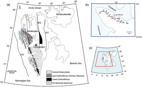
Here, we present MT data collected from Brøggerhalvøya (Fig. 1b), north-western Spitsbergen. The peninsula accommodates Ny-Ålesund, the closest year-round settlement to the North Pole, which we used for accessing the logistics necessary during the MT fieldwork. As shown in Fig. 1a, the data were collected in the broadband range from 13 stations along a curved WNW–ESE profile along a glacier-free plain (ca. 18 km) on the peninsula, facing the inlet of Kongsfjorden. The geological framework of the peninsula from surface to a few hundred metres depth is well established and characterized by a set of anomalous Tertiary fold–thrust sheets and subsequent extensional fault structures (Bergh et al. 2000; Saalmann & Thiedig 2002); however, the crustal structure at deeper levels is not well constrained. The presence of such a tectonically active subsurface in the vicinity of the settlement can be rewarding when it comes to a potential geothermal resources exploration.

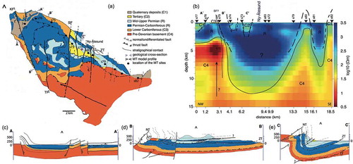
Figure 1. (a) The Svalbard Archipilago with its Tertiary affected section along the transform Hornsund Fault Zone (HFZ) highlighted. The map includes locations of Carboniferous basin strata: the Billefjorden Trough adjacent to the Billefjorden Fault Zone (BFZ), the Lomfjorden Fault zone (LFZ), Inner Hornsund Trough (IHT) and St. Jonsfjorden Trough (SJT). Note also the Tertiary Forlandsundet Graben just south of Brøggerhalvøya. The map is modified and redrawn from Bergh et al. (2000) and Saalmann & Thiedig (2002). (b) The MT studied area on Brøggerhalvøya, also represented in (a) and (c) with blue frames. The MT sites are indicated by the black dots and the pink dots denote sites with measured vertical magnetic fields in addition to the horizontal EM components. (c) The red box indicates the surface area of our 3D model.

In this paper, we extend the extent of the area on Svalbard covered by EM data (Beka et al. 2015; Beka et al. 2016) by interpreting the new MT data from Brøggerhalvøya using 3D inversion and by including the region’s bathymetry (Jakobsson et al. 2012) to account for coastal effects. As the amount of the available MT data is limited and the sites are measured along a single curved profile, we constrained the 3D model using a 2D model obtained from the impedance tensor determinant inversion. After comparing the preferred resistivity model with known bedrock lithology and structures (Bergh et al. 2000; Saalmann & Thiedig 2002), we use the final model to explore and discuss: (i) the deeper framework of the Tertiary fold–thrust belt along strike in a west–east cross-section; and (ii) the later-stage normal faults in section across their strike. By sketching the architecture of the upper crustal bedrock, the stratigraphical units beneath the Tertiary fold–thrust belt as well as the successive extensional fault systems, we discuss the relevance of the MT data in a regional context and make a reconnaissance assessment of the hidden geothermal potential near Ny-Ålesund.

Geological setting

The stratigraphy of Svalbard consists of a crystalline and metamorphic basement of Precambrian and Caledonian rocks overlain by a thick composite sedimentary sequence starting with Devonian and Carboniferous basin fills, and successive Permian through Eocene platform deposits up to 3.5 km thick (Harland 1997; Dallmann 1999). Notable thickness variations exist in the west–central and eastern parts of Svalbard for the Devonian basin deposits, but also for Carboniferous strata adjacent to reactivated block-boundary faults such as the Billefjorden and Lomfjorden fault zones (Harland 1997) as well as faults adjacent to the St. Jonsfjorden Trough in north-western Spitsbergen (Steel & Worsley 1984) and the Inner Hornsund Trough in southern part of Spitsbergen (Fig. 1a). In the Paleocene–Eocene a transpressional fold-and-thrust belt formed along the transform plate boundary between Greenland and the Barents Sea during break-up of the North-Atlantic Ocean (Harland 1997; Faleide et al. 2008), and affected large parts of western Spitsbergen, including the pre-Devonian and overlying sedimentary sequences (Dallmann et al. 1993; Bergh et al. 1997; Braathen et al. 1999).

On the peninsula of Brøggerhalvøya (Challinor 1967; Hjelle 1999) the Tertiary fold–thrust belt consists of three major, north–north-east-vergent basement-involved fold–thrust sheets (lower, middle and upper nappes) cut by younger normal and strike–slip faults trending north–south (Bergh et al. 2000; Saalmann & Thiedig 2002). The pre-Devonian strata consist of various low-grade metamorphic schists, meta-sandstones, quartzites, marbles and some gneisses, and are partly thrusted over younger Palaeozoic and Mesozoic strata in the south-east (Cutbill & Challinor 1965). In the western part of the peninsula, a less deformed sequence of competent Carboniferous sandstones and Lower Permian carbonates (limestone, dolomite) are exposed in the near surface. In the central and northern parts of the peninsula, in the Ny-Ålesund area, younger Triassic–Paleocene–Eocene sandstones and coal-bearing deposits are preserved in a major syncline of the middle nappe, overlying the repeated/thickened Carboniferous–Permian units of the lower nappe. The youngest, north–south trending and steeply dipping normal/strike–slip faults of the area display kilometre-scale vertical down-faulting of the sedimentary strata (e.g., the Scheteligfjellet Fault) and cause variable lateral offset and segmentation of the fold–thrust structures (Bergh et al. 2000), which we further assess using the MT data.

Methods

Magnetotellurics is a plane wave EM geophysical method that enables the resistivity structure of the subsurface to be derived from measured natural source electric and magnetic fields at the surface of the earth (Tikhonov 1950; Cagniard 1953). In the frequency domain, the measured horizontal electric (E_x,E_y) and magnetic (H_x,H_y) field components are linearly related through a transfer function that is refereed to as the impedance tensor, Z.

(1)

Under a homogeneous plane wave condition, Z depends on the underlying resistivity structure (Berdichevsky 1960; Chave & Jones 2012). Similarly, in the frequency domain, the magnetic field vertical component (H_z) is linked to H_x and H_y through a transfer function often called tipper, T (Vozoff 1972):

(2)

In particular, tippers are more sensitive to the surrounding 3D conductivity structure and can provide valuable information on lateral resistivity variations (Simpson & Bahr 2005). Tippers can be visualized as induction arrows, helping to identify locations of large conductive zones and assisting in defining the direction of strike in a 2D condition (Chave & Jones 2012; Samrock et al. 2015).

Data acquisition

We recorded the MT data on Brøggerhalvøya at 13 stations (s71–s83) along the Kongsfjorden inlet (Fig. 1a). Besides the horizontal EM fields, we also measured the vertical magnetic field at five of the stations to derive induction arrows. When picking a site, we tried to avoid areas that were steep or covered in deep snow. As a result the site-to-site separation varied between 500 m and 2000 m.

The data were recorded in the 0.003 – 1000 s period range using the MTU2000 MT system (Smirnov et al. 2008). For magnetic fields measurement, we used LEMI-120 broadband induction coil magnetometers produced in Ukraine. Electric fields are measured using two orthogonal dipoles aligned with magnetic north–south and east–west directions, and typically with a ca. 100 m long wire having non-polarizable Pb-PbCl₂ electrodes at each end. At each station, data were recorded for about 24 hours in dual sampling burst modes. Sampling at 20 Hz was performed during the entire data acquisition, and at midnight when in general low industrial noise was anticipated a simultaneous 1000 Hz sampling was carried out for 2 hours for burst recording. Data loggers were connected to a GPS receiver for the purpose of accurate time synchronization between stations operating simultaneously and for precise determination of station location.

During data recording, we installed two to three instruments at a time at different locations for simultaneous recording so that the data from one station could be used as a remote reference for the others (Smirnov et al. 2008). We measured all the MT sites in the month of May in 2015, when snow conditions allowed travel by snowmobiles and the temperature was not far below freezing, avoiding instrument malfunctioning. The remoteness of the studied area from industrial noise guaranteed high-data quality. Despite the threat of data bias due to proximity of the studied location to ionospheric sources (Viljanen et al. 1999; Simpson & Bahr 2005; Chave & Jones 2012), we have not noticed irregularity in the measured broadband data that we can relate to source field effects. Furthermore, the depth level we are interested in is much smaller than the typical distance to the sources, ca. 100–120 km (Sahr et al. 1991). We can therefore assume that the plane wave condition for the depth of interest is satisfied.

We processed the measured time-varying electric and magnetic field data using the Robust Remote Reference Algorithm of Smirnov (2003), where final results were derived through averaging multiple remote reference estimates in a robust statistical manner (Smirnov & Pedersen 2009).

Strike and dimensionality analysis

Prior to data inversion, it is necessary to understand the geoelectric strike and dimensionality situation of the data in order to avoid model distortions. For the analyses, we employed the phase tensor (Φ) method (Caldwell et al. 2004), which is considered to be immune to galvanic distortions arising from near surface conductivity heterogeneities (Jiracek 1990).

The phase tensor (Φ = X⁻¹Y) is derived from the impedance tensor’s real (X) and imaginary (Y) parts. Φ can be expressed in a decomposed form in terms of three coordinate invariants (i.e., the tensor’s maximum ϕ_max, minimum ϕ_min and the skew angle β) together with an auxiliary angle α defining the tensor’s dependence on the coordinate frame:

(3)

R(α + β) is a rotation matrix and the superscript denotes its transpose. The skew angle β measures the tensor’s asymmetry. β less than three degrees could be used as a subjective criterion for a 2D Earth (Booker 2014). Ellipses provide a graphical illustration of the tensor, where the ellipse’s major and minor axes depict its principal axes, and orientation of the major axis is specified by α − β, which also gives an estimate of the geo-electric strike (Caldwell et al. 2004; Booker 2014).

In Fig. 2a we illustrate the phase tensor ellipses of the 13 sites we measured, sorted in a WNW–ESE direction, together with their corresponding skew angles in colour fills, as a function of period. The skew angles (β^∗ ) are presented having their errors (Chave & Jones 2012; Booker 2014) taken into account following a bootstrapping technique (Efron & Tibshirani 1994) suggested by Cherevatova et al. (2015), where the standard error obtained through 1000 bootstrap realizations is removed, to present only the significant part of the skew angle associated with deviation from the underlying 2D assumption.

The phase tensor ellipse diagram we present in Fig. 2a can be seen as having five zones with some collective behaviour between 0.003 s and 1000 s, on the basis of their geometry and skew. Below we discuss the following period intervals shown in Fig. 2: (i) 0.003–0.1 s, (ii) 0.1–1 s, (iii) 1–10 s, (iv) 10–100 s, and (v) 100–1000 s.

Figure 2. Geoelectric strike and dimensionality. (a) Phase tensor ellipses of the 13 measured sites with their error accounted skew angles (β^∗ ) in colour fills. (b – e) Phase tensor strike estimates for period intervals manifesting a collective dimensionality behaviour. (f) Phase tensor strike estimate for the entire data set (0.003–1000 s). The analysis in general indicates strong 3D effects, with some localized underlying 2D structures and a weak regionally dominant strike direction suitable for the entire data set.

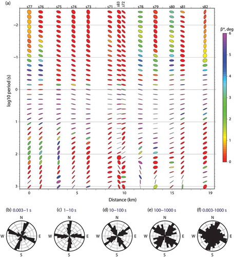
In zone (i), the ellipses display a circular geometry that is consistent with a 1D situation. In addition, the skew angles indicate values that are nearly zero or less than three degrees along the profile, which again support the proposed 1D situation. In zone (ii), the ellipses are less circular, and the skews are larger than three degrees at a number of sites (s77, s76, and s78–s82), which may indicate some 3D effect. As a comparison, we displayed the phase tensor strike estimated for zone (i) and (ii) together in Fig. 2b. The rose diagram of the estimate indicates a dominant strike at about N15E–N30E (with 90 degree ambiguity) for the section. For further justification of the strike and dimensionality condition, Fig. 3 illustrates the real part of the induction arrows derived from the tipper data in Wiese convention (Wiese 1965), where arrows point away from a conductor. Panel (a) of this figure displays the induction arrows at 1 s, where there is a good coincidence between the phase tensor estimated strike direction and the arrow’s collective orientation. Besides supporting the strike estimate (ca. N20E), the arrows also display large magnitudes. We conclude that in zone (i) and (ii) the structure can be better explained as 2D but with 3D effects superimposed. In interval (iii), the geometry of the ellipses is dominated by the major axes, with different rotations at the western (s77–s78) and eastern (s80–s82) sections of the profile. The skew angles of the zone display mostly values larger than three degrees indicating 3D effects, whereas strike estimated (Fig. 2c) for the zone indicated a dominant north–south-trending strike with 90 degrees ambiguity. On the other hand, induction arrows from the period interval plotted on Fig. 3b for 8 s indicate two different orientations, north–south for the eastern and ca. N120E for the western section, with small arrow magnitudes. This indicates that there is no consistent strike suitable for the entire profile. We conclude that, besides having a notable 3D effect, zone (iii) has no consistent strike suitable for the entire profile. In zone (iv), the major axes of the ellipses still dominate but compared to the previous zone, the major axes are collectively rotated clockwise, and there are several sites with nearly zero skew values. Besides, the zone’s strike estimate (Fig. 2d) and the collective orientation of the arrow at 64s (Fig. 3c) both support a dominant strike of about N60E. We consider most of the structures in zone (iv) can be explained with a 2D model.

Figure 3. Real part of the induction arrows of the sites s71, s83, s72, s81 and s82 respectively in north-west–south-east direction, in Wiese convention. The arrows are plotted for 1, 8, 64 and 724 seconds in (a) through (d), respectively. The strike directions indicated by the arrows display a reasonable match with the phase tensor strike estimates shown in Fig. 2b–e.

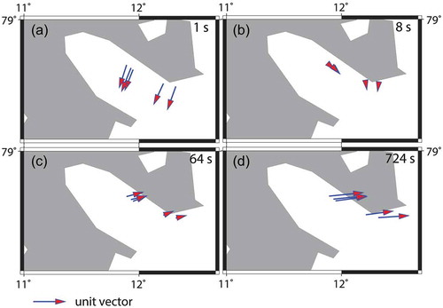
In zone (v), despite mostly small (<3) skew angles, the phase tensor ellipses indicate chaotic geometry particularly in the eastern section of the profile between s83 and s82. This is well reflected on the zone’s strike estimate shown in Fig. 2e, where it was difficult to find a single direction suitable for the period interval. The induction arrows from the zone shown on Fig. 3d display a more collective behaviour with large magnitudes. However, there is also an indication of a minor rotation of the orientation between s81 and s82 (last two tipper sites towards east). Finally, the dimensionality analysis suggests the presence of a weak regional level N20E strike that could be suitable for the entire data set, as can be seen in Fig. 2f. To conclude, the data have 3D behaviour as a whole; nonetheless, a tendency for localized 2D behaviour is also undeniable. Therefore, to obtain the full picture, data interpretation should be performed using 3D inversion and benchmarked with 2D modelling.

2D inversion

Two-dimensional modelling was performed to later benchmark 3D results, by inverting the apparent resistivities and the phase parameters of the determinant data in Occam’s manner (Constable et al. 1987), and seeking the smoothest model that reproduced the observed data using the Reduced Data Space Occam code (Siripunvaraporn & Egbert 2000). During the inversion, we aimed at achieving unity as a RMS misfit between the modelled and observed data, while fitting the data within its errors and within some specified error floor. We excluded stations s71 and s78, collected close to Ny-Ålesund, because of their low data quality, and inverted 11 stations’ data. For each station 19 data points were selected and used in the inversion. Inversion started from a homogeneous initial half-space model of 10 Ωm consisting of 66 cells in the horizontal and 98 cells in the vertical direction that correspond to a physical length of 248 370 km and 569 399 km, respectively. Air layers were not taken into account in the model since topography was out of the scope of the study. The central section of the model where the data sites were concentrated was gridded more densely than the edges, using cells ranging between 150 m and 400 m. This section was padded by subsequent cells that increase in size by a factor of 1.2 logarithmically towards the model edges. To ensure correct model scaling, the sites were projected onto a profile perpendicular to the assumed N20E regional strike based on the analysis discussed above.

Despite the weak regional-level strike (Fig. 2f), the dimensionality analysis discussed in the previous section also suggested strong 3D effects Fig. 2a) coupled with unstable strikes between period intervals (Fig. 2c–e). As a consequence, we could not adequately fit the customarily inverted TE+TM mode data in 2D. Even attempting to fit the TE and TM modes separately did not achieve RMS misfits lower than nine. Because of its rotationally invariance property the determinant is suitable for 2D inversion when MT profile data manifest 3D effects (Pedersen & Engels 2005). We employed the determinant as an alternative to the traditionally inverted bimodal data. 2D inversion was therefore performed mainly to later benchmark the 3D modelling result.

For the final 2D inversion, we assigned the error floors of 3% on the apparent resistivity and 0.015 rad (≈ 0.86 deg) on the phase parameters. The preferred 2D inversion model was obtained at the eighth iteration having 1.16 as an overall RMS misfit. The data misfit between the observed and predicted apparent resistivity and phase parameters is illustrated site by site in Fig. 4. The misfit curves display in general a good match between the observed and modelled data, except during long periods at a few sites (e.g., s72, s83, s79) where the data quality is lower, as the large errors indicate. The model itself is presented in Fig. 5b. The overall geometry of the main anomalies displayed on preferred 2D model (Fig. 5b) seemed to be consistent and reproducible when the inversion was repeated and tested with other starting models and inversion algorithm (Kalscheuer et al. 2010).

Figure 4. The site by site data misfit between the observed (orange dots) and predicted (black solid lines) determinant data apparent resistivity (Ωm in log10 scale) and phase (deg) parameters underlying the preferred 2D inversion model displayed in Fig. 5b having 1.16 as its overall RMS misfit. All the modelled sites are included in the plot ordered from top – bottom right following the MT profile’s WNW–ESE direction. The y axes are given in log10 scales in seconds.

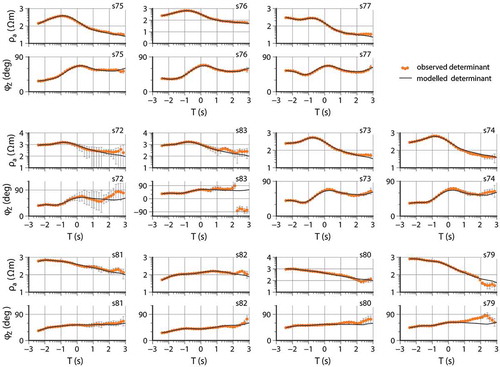
Figure 5. The preferred 2D MT model displayed together with bedrock geology for comparison. (a) A simplified surface geology map for Brøggerhalvøya illustrating the major fold–thrust belt structures and younger, crosscutting normal fault systems; simplified and redrawn from Bergh et al. (2000). (b) The 2D MT model. The MT model anomalies (R, C1 – C4) reasonably correspond with the geology and their interpretation is listed in the colour key in a coinciding manner with the bedrock map. Geological cross-sections that are redrawn from Bergh et al. (2000) are displayed in (c) through (e).

3D inversion strategy

It has been shown using synthetic data experiments that a more realistic image of subsurface resistivities can be achieved through MT profile data 3D inversion, when the profile data manifest strong 3D effects (Siripunvaraporn et al. 2005). This would be appropriate here, considering the 3D effects identified (Fig. 2a) and a successful previous experience with MT profile data 3D interpretation (Beka et al. 2016). To better accommodate for 3D features during the inversion, we included all the four components of the impedance tensor. To freely experiment with different inversion parametrization and regularizations, we employed the ModEM code (Kelbert et al. 2014) built for EM geophysical data inversion following the modular approach (Egbert & Kelbert 2012). The code has a parallel version (Meqbel 2009) that facilitates testing several inversion set-ups swiftly and concurrently, which we took advantage of through a high performance computing facility.

For the inversion, we employed a model consisting of 69, 52 and 44 cells, in X, Y and Z directions, respectively, yielding a total of 157 872 model parameters. The physical area covered by the modelling scheme is displayed in Fig. 1c. The top layer in the vertical direction was set to be 10 m thick and the sizes of the subsequent cells were allowed to increase by a factor of 1.2 with depth. The model did not take air layers into account. The central part of the model where the field data are located (area of interest) was divided densely and homogeneously with a 300 × 300 m grid cells. Outside the area of interest, the model is padded with nine outer cells. Data were rotated by −30 degrees to achieve better alignment between data profile and model grids.

Within the ModEM algorithm, we experimented with several inversions by imposing different data error floors (10, 5 and 3%), starting models (10 Ωm, 100 Ωm and 1000 Ωm) and regularization arrangements that we fixed in the model covariance matrix (Kelbert et al. 2014; Samrock et al. 2015; Beka et al. 2016). Among the tested inversion strategies, combining a 10 Ωm starting model with balanced standard smoothing (0.3) between cells and assigning 10% data error floor led to the preferred inversion result by providing 1.68 as an overall RMS misfit between the observed and predicted impedance data. The preferred model obtained from full impedance inversion is presented in Fig. 6. Most of the resistivity features on this model are as well supported by the 2D inversion result presented in the previous section (Fig. 5b). However, to better justify the resolved resistivity features, it is necessary to include bathymetry in the modelling to constrain the inversion and allow model correction. For this, we employed a 500 × 500 m resolution Arctic region sea depth chart (Jakobsson et al. 2012). From the chart, we extracted a section relevant to the 3D modelling domain following the approach discussed in Beka et al. (2016). The bathymetry extract was subdivided into blocks corresponding to the XY plain of the MT model cells, and averaging within each cell was made to obtain a representative sea depth estimate for the modelling purposes. In the preferred starting model (10 Ωm), the resistivity of cells submerged in seawater was replaced with 0.3 Ωm. Similarly, in ModEM’s model covariance matrix, we froze the smoothing of the submerged cells by masking their corresponding location. The preferred final 3D model for interpretation is presented in Fig. 7a. This model was obtained by including the bathymetry as discussed above, and inverting the full impedance together with the available tipper data by assuming 0.1 absolute errors on the tipper elements. Refer to the figure key to see which sites had tipper data. The overall RMS misfit of this model is 2.2, and the result is obtained after 253 iterations. It can be seen that including the tipper in the inversion has introduced additional complexity to the inversion reflected as an increased overall RMS misfit (2.2) compared to the RMS misfit of the impedance inversion (1.68) presented in Fig. 6.

Figure 6. The 3D resistivity model obtained by inverting all the four components of the impedance tensor. The model has an overall misfit RMS 1.68, obtained after 300 iterations. Data fits of the model are displayed site by site with black solid lines in Fig. 8.

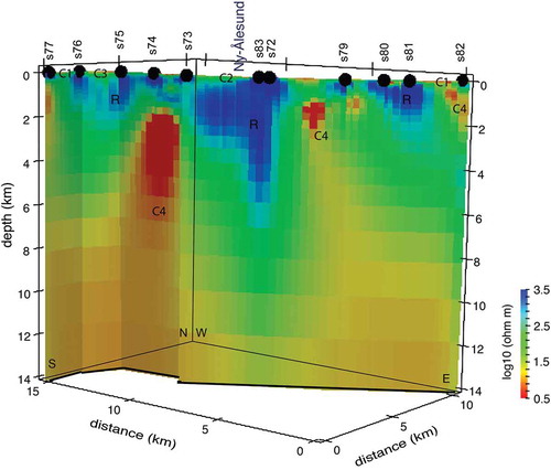
Figure 7. (a) The preferred final 3D model obtained by inverting the full impedance tensor by including detailed bathymetry and the tipper data. The 3D model is supported by the 2D result presented earlier and reflects a geologically meaningful reconstruction of the subsurface bedrock architecture. Interpretation of the model anomalies (R, C1 – C4) can be read from the colour key in Fig. 5. (b) Schematic presentation of the MT final model’s geological and structural interpretation along the studied WNW–ESE profile, showing a horst-graben geometry of alternating, uplifted pre-Devonian unit (C4) and down-faulted Permian–Carboniferous strata (C2 – C3, R).

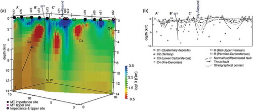
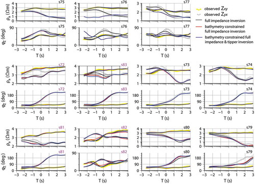
Figure 8. Data misfit between the observed data and results of three different 3D inversion procedures. The misfit is presented site by site for the observed Z_xy (yellow dots) and Z_yx (grey dots) impedance components in measurement coordinate system. The site names in purple represent the sites with the tipper data included in the inversion. For each site the apparent resistivity (Ωm) and the phase (deg) parameters are presented in the top and bottom panels, respectively. The data fit for the model presented in Fig. 6 (full impedance inversion; RMS = 1.68) is denoted with black solid lines, when bathymetry is included in the modelling (RMS = 2.17) in red solid lines and the final model (Fig. 7a, RMS = 2.2) data fits are shown with blue solid lines. The sites are ordered from top left to bottom right matching the MT profile’s WNW–ESE direction and in the same order as in Fig. 4.

In general, the final 3D inversion output (Fig. 7a) has reproduced the 2D (Fig. 5b) resistivity geometry, boosting the trustability of the 3D interpretation. Moreover, including bathymetry and tipper in the 3D enabled some minor corrections to be made to the 3D model obtained earlier by inverting the full impedances alone (Fig. 6). The misfit between the observed and 3D modelled apparent resistivity and phase parameters that were obtained from the inversions of the full impedance data alone, after bathymetry inclusion and after including the tipper data, are illustrated site by site in Fig. 8, in measurement coordinate system. It can be seen that, unlike the failed attempt to fit the data using bimodal 2D inversion, the 3D inversions provided satisfactory data fits. However, it was also obvious that there were some variabilities in the precision of the prediction from site to site. Particularly short period contents (≤10 s) of the data and sites west of s72 (i.e., sites closer to the coast) were more challenging to fit than the rest. Indication for a possible coast effect is also seen from s76’s fit, where bathymetry and tipper inclusion in the inversion equivalently produced a more conductive Z_yx component below ≤10 s. On the other hand, it is not clear why the inversions produce discrepancies for short periods at s72 and s83. However, one can speculate that the sites’ low data quality or the physical proximity between the two sites exceeding the 3D model resolution may account for the reduced precision achieved. In the next section, we present our interpretation based on the 3D final model (Fig. 7a), and by using the 2D result to support the conclusions. For simplicity, we name the anomalies in a similar manner across the 3D and 2D models.

Results

The final 3D (Fig. 7a) and 2D (Fig. 5b) MT models indicate a resistivity geometry that seem to reflect the structure and geological complexity of Brøggerhalvøya reported in previous studies (Challinor 1967; Bergh et al. 1997; Bergh et al. 2000; Saalmann & Thiedig 2002). For comparison with the MT models, the mapped surface geology (Bergh et al. 2000) together with three stratigraphic cross-sections are presented in Fig. 5a, c–e, respectively.

Taking into account the tectonic history of the region and correspondence to the geology, we grouped the major anomalies into four conductive parts (C1–C4) and a resistive section (R). Linking between the MT anomalies and the geology is given in Fig. 5a’s colour key. (i) C1 consists of shallow-level conductive features, from a combination of Quaternary deposits and the underlying Lower Carboniferous basin strata. It is observed at the north-west and south-east edges of the models. (ii) C2 represents the pools of shallow and relatively conductive sections present between s74 and s72. It is interpreted as possible signatures of the structurally uppermost and youngest (Tertiary) sedimentary rocks in the region. (iii) C3 represents the thin conductive segment in the near surface Fig. 5d. It is exposed between s76 and s75. The structure is interpreted as reflecting remains of the Lower Carboniferous strata. (iv) C4 represents a highly reworked and tectonically deformed deep conductive section, displayed beneath the resistive parts and seen as upraised domes between down-faulted resistors. The MT models indicate clearly that this pre-Devonian section, composed of low-grade metamorphic shales/schists and sandstones, is conductive, presumably arising from considerable vertical fluid and heat transport, particularly in the sections adjacent to the major faults. It is capped by directly overlaying resistive rocks. The resistivity in fault zones can be as low as tens of ohm-metres when composed of rocks fractured enough to host fluid migration that may lead to altered mineralogy (Eberhart-Phillips et al. 1995). (v) R represents the resistive section of the model with ca. 300 Ωm or more. The anomaly displays a belt like structure along the profile, with exposures at the surface and with locally varying thickness that ranges between ca. 1.5 and 5 km. The shallower section of R is considered to consist of a combination of multiple repeated (thrusted) Mid-Upper Permian successions, as well as a thick and repeated dolomite succession of the Upper Carboniferous/Lower Permian Wordiekammen Formation. The MT information make it difficult to distinguish between the successions of the Mid-Upper Permian and the Upper Carboniferous/Lower Permian, as both are resistive. On the other hand, the deeper section of R may be related to carbonate rocks in the basement with low fluid content leading to high resistivity (Palacky 1987). We provide further discussion of the shallow and deeper resistivity structure in the following paragraphs.

The shallow structure

At the shallow near-surface level, the MT model displays its longest highly resistive (ca. 1000 Ωm) lateral strip stretching approximately between s83 (near Ny-Ålesund) and s81, coinciding with the best exposures of Mid–Upper Permian carbonate formations of the mapped surface. To the east and west of the Ny-Ålesund area, also in agreement with the geological map, the near surface section of the MT model indicates transitions to relatively small conductive sections. These may represent the Tertiary sedimentary rocks (C2) around s73, and towards the eastern edge of the model either Quaternary deposits (C1) or a conductive pre-Devonian (C4) sliver thrusted over the Permian succession (R) in the middle nappe below and/or in the upper nappe (Bergh et al. 2000; Saalmann & Thiedig 2002). Another striking feature of the 2D MT model is signatures of the younger normal faults that truncate the fold–thrust belt structures. For instance, the two faults that may have down-dropped the Permian strata and allowed the pre-Devonian strata to retain closer to the surface are well marked to the left and right of the site s80, although this is not clear from the 3D model. In another example, the model suggests C4 protruding to the near surface just east of s82, in the vicinity of second major normal fault. At a similar location, there is geological evidence for the pre-Devonian reaching to the surface, as Fig. 5a indicates.

The deeper structure

At a deeper level, the resistive anomaly (R) of ca. 500–3000 Ωm is imaged dipping up to 5 km beneath the Ny-Ålesund area and reaching at most to a depth of 2 km at other locations along the profile. The deepest sections of R occur where previous geological studies indicated vertically the most complete post-Devonian succession, repeated by thrust faults and folded into a major syncline with steeply dipping Permian-Carboniferous succession on the fold limbs consisting of thick and repeated resistive dolomite successions, as illustrated by the cross-section C–C’ in Fig. 5e. However, presence of such a resistive Permian dolomites at depth scale >5 km on the 2D model is unlikely and must be accounted for, for instance, by carbonate rocks in the basement. Moreover, the long period sections of the data for the sites s72 and s82 corresponding the area of the deepest R have poorer quality and data fits (see Fig. 4), making the resolved structure less trustable.

Further to the north-west, below s74 and s73, the model indicates shallower siliciclastic units (e.g., Tertiary formations) bounded by faults and folds as signified by Fig. 5a, e close to the surface. Clearly the most conductive (<10 Ωm) anomaly appears at about 4–6 km depth underneath a presumed steep/subvertical fault that cross-cuts the model just to the east of s74. This structure overlaps with the mapped Scheteligfjellet Fault (Fig. 5a), a late-stage normal fault a vertical throw-down to the east of up to 1 km, and with an additional strike–slip component. This fault may have facilitated upward fluid and heat transport within the adjacent shallower seated pre-Devonian unit in the foot-wall of the Scheteligfjellet Fault to the west, creating a sealed aquifer like structure possibly originating from intruded seawater and imaged as a highly conductive anomaly (<10 Ωm) between ca. 3.5 km and 7 km depth beneath s74 and extending towards s77. To control its reliability and lateral extent, and to check whether the data have enough resolution to image this aquifer like structure, we performed sensitivity tests in 2D. For the tests, we replaced the section on the final model between 3.5 km and 7 km depth and beneath s77–s74 with: (i) 50 Ωm to resemble the conductive background below it; (ii) 200 Ωm to prolong the semi-resistive part imaged directly east of it; and (iii) 2000 Ωm aiming at extending the resistive anomaly imaged overlying the aquifer. After perturbing the final 2D model in the above three ways, we carried out forward modelling using each of the altered models as an input, and assessed the impact on the final model’s data misfit RMS (1.16). All three test scenarios increased the overall data misfit RMS, mainly produced by severely under-fitted sites between s77 and s74 after the perturbation. The new values of the overall misfit RMS were 2.29, 2.8 and 3.1, respectively for the first, second and third test scenarios. Among the MT sites, s76 in particular could not be fitted, having 5.3 and 2.9 as its apparent resistivity and phase misfit RMS during the first test. This is also in line with the 3D inversion result for s76 where a rather conductive short period section is estimated when bathymetry and tipper were included in the inversion (see Fig. 8). On the basis of the sensitivity test results, we can conclude that the data sense the aquifer and that it may extend laterally towards the west.

The position of the sub-vertical SF and the associated conductive aquifer is slightly shifted towards the east in the 3D model. The placement of Scheteligfjellet Fault between s74 and s73 overlaps well with the actual position of the fault as indicated on Fig. 5a. Moreover, the 3D model suggests a seemingly uplifted conductive section at about 3–6 km depth east of the Scheteligfjellet Fault, between s73 and s71. The newly resolved conductive anomaly is interpreted as a signature of a combined down-faulting and strike–slip displacement of Pre-Devonian and cover rocks in the hanging wall of the Scheteligfjellet Fault (Fig. 5a). A peculiar feature of this conductive anomaly is that the conductor seems laterally well sealed by steeply-dipping resistive sections, and the resistive cap-rock on top of the structure is thicker than the presumed aquifer at a similar depth to the east in the footwall of Scheteligfjellet Fault under s74. This may also support the known thrust–fault repetitions of the Pre-Devonian sheets in the thrust stack seen further north on the peninsula, as the cross-section B–B’ in Fig. 5d indicates. However, we also recognize that such a resistivity feature may also be an effect of model regularization. Furthermore, sharp and more vertical dip of the resistive part beneath s82 and s72 correlates well with the increased dip of the folded Permian–Carboniferous formations as illustrated in Fig. 5e. Towards the westernmost part of the model, between s75 and s77, both the final 3D and 2D models indicate a thinned resistive section, which may have resulted from extensive erosion at this coastal part, where a vast quantity of Quaternary fluvial and glacial deposits are present.

Discussion

Reliability of the MT results

Besides extending the EM data coverage on Svalbard, the newly collected MT data from Brøggerhalvøya provides geologically meaningful and valuable information on the crustal framework of the Tertiary affected western part of the archipelago (Fig. 1a). Inverting the MT impedance data in 2D (Fig. 5b) and 3D (Fig. 6) provided in general comparable results.

However, despite an overall satisfactory RMS misfits both from the 3D (1.68) and 2D (1.18) MT impedance data inversions, it was relatively challenging to fit short period ranges of the data in 3D and longer period ranges in 2D. The challenge was in particular encountered at sites closer to coast (e.g., s76) and for sites having lower data quality (e.g., s72 and s83) as indicated in Figs. 4 and 8b. The poor fit to sites s72 and s83 may be because the sites are simply too close and lack sufficient resolution for the 3D scheme, or that the data quality in this tectonically complex section of the profile around Ny-Ålesund is not good enough, noting that two other sites (s71 and s78) from this section are already excluded from the inversion because of their bad quality. Geologically, this section is associated with a complex fold-and-thrust system (Fig. 5a), where there is indication for the presence of a steeply dipping Permian–Carboniferous succession (Fig. 5e) that corresponds well with the 3D model predictions (Figs. 6, 7) where a resistive structure is shown beneath s83 and s72. The 2D model is carefully tested for sensitivity through re-running the inversion with a different algorithm and by starting inversions with different starting models and assessing the reproducibility of the major anomalies. In general, the 2D model adequately supports the final 3D model except in the near surface 200 m section, where the 3D models display a slightly less resistive and less comparable structure to the known surface geology (Fig. 5a).

Geological relevance of the MT model

The presented MT final 3D model nicely documents in some detail the conclusions drawn from geological surface mapping (Fig. 5a) down to 1–3 km depth in Brøggerhalvøya (Hjelle 1999; Bergh et al. 2000; Saalmann & Thiedig 2002). First, it supports the occurrence of a highly reworked pre-Devonian basement overlain by dominantly resistive sedimentary rocks (carbonate-rich Carboniferous and Permian strata) that are involved in the crustal-scale north–north-east-vergent Tertiary fold–thrust belt. However, since the strike of the tilted bed rocks are mostly parallel to the MT profile, geometry of the fold–thrust belt structures is not well constrained. On the other hand, the pronounced thickness of the resistive parts of the model (Carboniferous–Permian carbonates) supports crustal shortening and repetition by thrust faulting. Alternatively, the depth increase of the resistive unit may arise from a hidden Carboniferous basin below the thrust stack (i.e., Brøggerhalvøya basin) linked, for example, to the Carboniferous St Jonsfjorden Trough farther south (Cutbill & Challinor 1965; Worsley 2008), a feature also inferred by Bergh et al. (2000). Secondly, the deep resistive anomaly (R, 3–5 km depth) may represent carbonate rocks in the basement. Thirdly, and more convincing, the geological interpretation of the MT model shown in Fig. 7b in a WNW–ESE section, resembles that of a complex horst/ridge (pre-Devonian) and graben/depression (Carboniferous and Permian) system, formed by dominantly extensional normal and subordinate, strike–slip down-faulting perpendicular to the fold–thrust belt structures (Fig. 5a). This model favours a sequential interplay between the WNW–ESE trending Tertiary fold–thrust belt structures and later Paleocene–Eocene east–west-directed normal and transform faulting, i.e. that first thickened the resistive (Carboniferous and Permian) portion of the crust, and later extended the pre-Devonian crust. This is a feature also known to occur farther south-eastward along the Tertiary affected portions of mainland Spitsbergen (Dallmann et al. 1993; Harland 1997; Braathen et al. 1999). Furthermore, the horst-graben model inferred from the MT data supports a southward link with the known Tertiary Forlandsundet graben (Gabrielsen et al. 1992) as well as onshore transform faults (Maher et al. 1997; Braathen et al. 1999). Finally, the anomaly portions of the MT model, for example, irregular clusters of conductive units within resistive middle and upper-level resistive sections suggest a complex relationship between upthrusted, repeated pre-Devonian successions and down-faulted blocks of Carboniferous and Permian rocks, in conjunction with variable crustal rheology, complex lithology/stratigraphy and various crustal and surficial processes.

Conclusion

Using MT and tipper data sets collected recently on Brøggerhalvøya (north-west Svalbard), we analysed the surface-crustal-level geology of the region along a WNW–ESE profile. The data were modelled in 2D and 3D, and the resulting geometry reflected well the known bedrock geology and tectonics structure. The new MT data have contributed to unravelling both the shallow and the deeper architecture of the crustal geology of western Spitsbergen, which have heretofore not been well studied. The MT data imaged interplay between repeated and reworked basement-involved fold–thrust belt structures and successive steeply dipping oblique-normal faults (e.g., the Scheteligfjellet Fault) that created a basement-seated horst/ridge and graben/depression system. The MT models (2D and 3D) indicated aquifers within the upraised horsts of pre-Devonian shale/schist unit at ca. 2–6 km depth in the vicinity of the sub-vertical Scheteligfjellet Fault. Since there is also evidence for a lateral and sub-vertical cap-rock sealing at the same location surrounding the aquifer systems, this area seems to be the most appropriate to investigate more closely for exploitable geothermal heat.

To conclude, the MT model suggests a highly conductive shallow-mid crust basement-cover architecture with thick resistive carbonate rocks and Tertiary fold–thrust belt structures, down-dropped by later oblique normal faults. At deeper levels, the model shows that these normal faults in the pre-Devonian basement may provide a clear trace for fluid and heat migration towards the surface.

Acknowledgments

The authors thank the Norwegian Ministry of Foreign Affairs for supporting the field survey. We are grateful to Oulu University, Finland, for lending MT instruments. We also acknowledge support from UNINETT in making computation resources available under the quota system NN9362K at the Stallo high performance computing facility at the UiT – The Arctic University of Norway. We greatly appreciate the constructive comments provided by Xavier Garcia, an anonymous reviewer and the journal’s Section Editor Robert Spielhagen for helping us to improve the manuscript.

Disclosure statement

No potential conflict of interest was reported by the authors.

Additional information

Funding

This work was supported by the Norwegian Ministry of Foreign Affairs.

References

- Bælum K. & Braathen A. 2012. Along-strike changes in fault array and rift basin geometry of the Carboniferous Billefjorden Trough, Svalbard, Norway. Tectonophysics 546, 1–14.
- Beka T.I., Senger K., Autio U.A., Smirnov M. & Birkelund Y. 2017. Integrated electromagnetic data investigation of a Mesozoic CO2 storage target reservoir-cap-rock succession, Svalbard. Journal of Applied Geophysics 136, 417–430.
- Beka T.I., Smirnov M., Bergh S.G. & Birkelund Y. 2015. The first magnetotelluric image of the lithospheric-scale geological architecture in central Svalbard, Arctic Norway. Polar Research 34, article no. 26766, doi: 10.3402/polar.v34.26766
- Beka T.I., Smirnov M., Birkelund Y., Senger K. & Bergh S.G. 2016. Analysis and 3D inversion of magnetotelluric crooked profile data from central Svalbard for geothermal application. Tectonophysics 686, 98–115.
- Berdichevsky M. 1960. Principles of magnetotelluric profiling theory. Applied Geophysics 28, 70–91.
- Bergh S.G., Braathen A. & Andresen A. 1997. Interaction of basement-involved and thin-skinned tectonism in the Tertiary fold–thrust belt of central Spitsbergen, Svalbard. The American Association of Petroleum Geologists Bulletin 81, 637–661.
- Bergh S.G. & Grogan P. 2003. Tertiary structure of the Sorkapp–Hornsund region, south Spitsbergen, and implications for the offshore southern extension of the fold–thrust belt. Norwegian Journal of Geology 83, 43–60.
- Bergh S.G., Maher H.D. & Braathen A. 2000. Tertiary divergent thrust directions from partitioned transpression, Brøggerhalvøya, Spitsbergen. Norwegian Journal of Geology 80, 63–81.
- Blinova M., Faleide J.I., Gabrielsen R.H. & Mjelde R. 2012. Seafloor expression and shallow structure of a fold-and-thrust system, Isfjorden, west Spitsbergen. Polar Research, 31, article no. 11209, doi: 10.3402/polar.v31i0.11209
- Booker J.R. 2014. The magnetotelluric phase tensor: a critical review. Surveys in Geophysics 35, 7–40.
- Braathen A., Bergh S.G. & Maher H.D. 1999. Application of a critical wedge taper model to the Tertiary transpressional fold–thrust belt on Spitsbergen, Svalbard. Geological Society of America Bulletin 111, 1468–1485.
- Cagniard L. 1953. Basic theory of the magnetotelluric method of geophysical prospecting. Geophysics 18, 605–635.
- Caldwell T.G., Bibby H.M. & Brown C. 2004. The magnetotelluric phase tensor. Geophysical Journal International 158, 457–469.
- Challinor A. 1967. The structure of Brøggerhalvøya, Spitsbergen. Geological Magazine 104, 322–336.
- Chave A.D. & Jones A.G. 2012. The magnetotelluric method: theory and practice. Cambridge: Cambridge University Press.
- Cherevatova M., Smirnov M.Y., Jones A., Pedersen L., Group M.W., Beckan M., Biolik M., Cherevatova M., Ebbing J., Gradmann S., Gurk M., Hubert J., Jones A.G., Junge A., Kamm J., Korja T., Il L., Lower A., Nigginger C., Pedersen L.B., Savvaidis A. & Smirnov M. 2015. Magnetotelluric array data analysis from north-west Fennoscandia. Tectonophysics 653, 1–19.
- Constable S.C., Parker R.L. & Constable C.G. 1987. Occam’s inversion: a practical algorithm for generating smooth models from electromagnetic sounding data. Geophysics 52, 289–300.
- Cutbill J. & Challinor A. 1965. Revision of the stratigraphical scheme for the Carboniferous and Permian rocks of Spitsbergen and Bjørnøya. Geological Magazine 102, 418–439.
- Dallmann W.K. 1999. Lithostratigraphic lexicon of Svalbard. Tromsø: Norwegian Polar Institute.
- Dallmann W.K., Andresen A., Bergh S.G., Maher H.D.J. & Ohta Y. 1993. Tertiary fold-and-thrust belt of Spitsbergen, Svalbard. Meddelelser 128. Oslo: Norwegian Polar Institute.
- Eberhart-Phillips D., Stanley W.D., Rodriguez B.D. & Lutter W.J. 1995. Surface seismic and electrical methods to detect fluids related to faulting. Journal of Geophysical Research—Solid Earth 100, 12919–12936.
- Efron B. & Tibshirani R.J. 1994. An introduction to the bootstrap. Boca Raton: CRC Press.
- Egbert G.D. & Kelbert A. 2012. Computational recipes for electromagnetic inverse problems. Geophysical Journal International 189, 251–267.
- Eiken O. 1994. Seismic atlas of western Svalbard. Meddelelser 130. Oslo: Norwegian Polar Institute.
- Faleide J.I., Tsikalas F., Breivik A.J., Mjelde R., Ritzmann O., Engen O., Wilson J. & Eldholm O. 2008. Structure and evolution of the continental margin off Norway and the Barents Sea. Episodes 31, 82–91.
- Gabrielsen R.H., Kløvjan O.B.S., Haugsbø H., Midbøe P.S., Nøttvedt A., Rasmussen E. & Skott P.H. 1992. A structural outline of Forlandsundet Graben, Prins Karls Forland, Svalbard. Norwegian Journal of Geology 72, 105–120.
- Haremo P., Andresen A., Dypvik H., Nagy J., Elverhøi A., Eikeland T.A. & Johansen H. 1990. Structural development along the Billefjorden Fault Zone in the area between Kjellstrømdalen and Adventdalen/Sassendalen, central Spitsbergen. Polar Research 8, 195–216.
- Harland W.B. 1997. The geology of Svalbard. London: Geological Society.
- Hjelle A. 1999. Geological map of Svalbard 1:100 000. Sheet A7G Kongsfjorden. Tromsø: Norwegian Polar Institute.
- Jakobsson M., Mayer L., Coakley B., Dowdeswell J.A., Forbes S., Fridman B., Hodnesdal H., Noormets R., Pedersen R., Rebesco M., Schenke H.W., Zaraskaya Y., Acetella D., Armstrong A., Anderson R.M., Edwards M., Gardner J.V., Hall J.K., Hell B., Bestvik O., Kristoffersen Y., Marcussen C., Mohammed R., Mosher D., Nghiem S.V., Pedrosa M.T., Travaglini P.G & Weatherall P. 2012. The International Bathymetric Chart of the Arctic Ocean (IBCAO) version 3.0. Geophysical Research Letters 39, L12609, doi: 10.1029/2012GL052219
- Jiracek G.R. 1990. Near-surface and topographic distortions in electromagnetic induction. Surveys in Geophysics 11, 163–203.
- Kalscheuer T., Juanatey D.Á.G., Meqbel N. & Pedersen L.B. 2010. Non-linear model error and resolution properties from two-dimensional single and joint inversions of direct current resistivity and radiomagnetotelluric data. Geophysical Journal International 182, 1174–1188.
- Kelbert A., Meqbel N., Egbert G.D. & Tandon K. 2014. ModEM: a modular system for inversion of electromagnetic geophysical data. Computers & Geosciences 66, 40–53.
- Khutorskoi M., Leonov Y.G., Ermakov A. & Akhmedzyanov V. 2009. Abnormal heat flow and the trough’s nature in the northern Svalbard plate. Doklady Earth Sciences 424, 29–35.
- Maher H.D., Bergh S., Braathen A. & Ohta Y. 1997. Svartfjella, Eidembukta, and Daudmannsodden lineament: tertiary orogen-parallel motion in the crystalline hinterland of Spitsbergen’s fold–thrust belt. Tectonics 16, 88–106.
- Meqbel N.M.M. 2009. The electrical conductivity structure of the Dead Sea Basin derived from 2D and 3D inversion of magnetotelluric data. PhD thesis, Freie Universität Berlin, Germany.
- Palacky G. 1987. Resistivity characteristics of geologic targets. In: M.N. Nabighian (ed.): Electromagnetic methods in applied geophysics. Pp. 53–129. Tulsa: Society of Exploration Geophysicists.
- Pedersen L.B. & Engels M. 2005. Routine 2D inversion of magnetotelluric data using the determinant of the impedance tensor. Geophysics 70, G33–G41.
- Saalmann K. & Thiedig F. 2002. Thrust tectonics on Brøggerhalvøya and their relationship to the Tertiary West Spitsbergen Fold-and-Thrust Belt. Geological Magazine 139, 47–72.
- Sahr J.D., Farley D.T., Swartz W.E. & Providakes J.F. 1991. The altitude of type 3 auroral irregularities: radar interferometer observations and implications. Journal of Geophysical Research—Space Physics 96, 17805–17811.
- Samrock F., Kuvshinov A., Bakker J., Jackson A. & Fisseha S. 2015. 3-D analysis and interpretation of magnetotelluric data from the Aluto-Langano geothermal field, Ethiopia. Geophysical Journal International 202, 1923–1948.
- Simpson F. & Bahr K. 2005. Practical magnetotellurics. Cambridge: Cambridge University Press.
- Siripunvaraporn W. & Egbert G. 2000. An efficient data-subspace inversion method for 2-D magnetotelluric data. Geophysics 65, 791–803.
- Siripunvaraporn W., Egbert G. & Uyeshima M. 2005. Interpretation of two-dimensional magnetotelluric profile data with three-dimensional inversion: synthetic examples. Geophysical Journal International 160, 804–814.
- Slagstad T., Balling N., Elvebakk H., Midttømme K., Olesen O., Olsen L. & Pascal C. 2009. Heat-flow measurements in Late Palaeoproterozoic to Permian geological provinces in south and central Norway and a new heat-flow map of Fennoscandia and the Norwegian–greenland Sea. Tectonophysics 473, 341–361.
- Smirnov M., Korja T., Dynesius L., Pedersen L.B. & Laukkanen E. 2008. Broadband magnetotelluric instruments for near-surface and lithospheric studies of electrical conductivity: a Fennoscandian pool of magnetotelluric instruments. Geophysica 44, 31–44.
- Smirnov M.Y. 2003. Magnetotelluric data processing with a robust statistical procedure having a high breakdown point. Geophysical Journal International 152, 1–7.
- Smirnov M.Y. & Pedersen L.B. 2009. Magnetotelluric measurements across the Sorgenfrei-Tornquist Zone in southern Sweden and Denmark. Geophysical Journal International 176, 443–456.
- Steel R.J. & Worsley D. 1984. Svalbard’s post-Caledonian strata-an atlas of sedimentational patterns and palaeogeographic evolution. In A.M. Spencer et al. (eds.): Petroleum geology of the North European margin. Pp. 109–135. London: Graham & Trotman.
- Tikhonov A. 1950. On determining electrical characteristics of the deep layers of the Earth’s crust. Doklady Akademii Nauk 73, 295–297.
- Vågnes E. & Amundsen H.E.F. 1993. Late Cenozoic uplift and volcanism on Spitsbergen: caused by mantle convection? Geology 21, 251–254.
- Viljanen A., Pirjola R. & Amm O. 1999. Magnetotelluric source effect due to 3D ionospheric current systems using the complex image method for 1D conductivity structures. Earth Planets Space 51, 933–945.
- Vozoff K. 1972. The magnetotelluric method in the exploration of sedimentary basins. Geophysics 37, 98–141.
- Wiese H. 1965. Geomagnetische Induktionspfeile in der ČSSR, Hervorgerufen durch Grossräumige Elektrische Leitfähigkeitsstrukturen. (Geomagnetic induction arrows in the CSSR, caused by large-scale electrical conductivity structures.) Studia Geophysica et Geodaetica 9, 415–419.
- Worsley D. 2008. The post-Caledonian development of Svalbard and the western Barents Sea. Polar Research 27, 298–317.