Development of time series stacks of Landsat images for reconstructing forest disturbance history

Abstract

Forest dynamics is highly relevant to a broad range of earth science studies, many of which have geographic coverage ranging from regional to global scales. While the temporally dense Landsat acquisitions available in many regions provide a unique opportunity for understanding forest disturbance history dating back to 1972, large quantities of Landsat images will need to be analysed for studies at regional to global scales. This will not only require effective change detection algorithms, but also highly automated, high level preprocessing capabilities to produce images with subpixel geolocation accuracies and best achievable radiometric consistency, a status called imagery-ready-to-use (IRU). This paper describes a streamlined approach for producing IRU quality Landsat time series stacks (LTSS). This approach consists of an image selection protocol, high level preprocessing algorithms and IRU quality verification procedures. The high level preprocessing algorithms include updated radiometric calibration and atmospheric correction for calculating surface reflectance and precision registration and orthorectification routines for improving geolocation accuracy. These automated routines have been implemented in the Landsat Ecosystem Disturbance Adaptive System (LEDAPS) designed for processing large quantities of Landsat images. Some characteristics of the LTSS developed using this approach are discussed.

Keywords:

• Landsat time series stack
• imagery-ready-to-use
• LEDAPS
• forest change

1. Introduction

Comprising only about 40% of the ice-free land surface, forest contains nearly 80% of the total carbon estimated to be in the terrestrial aboveground biosphere (Waring and Running 1998). Forest disturbance and regrowth processes control the carbon residence time in the terrestrial biosphere and the net carbon flux between the biosphere and the atmosphere (Hirsch et al. 2004, Law et al. 2004). Knowledge of the history of forest disturbance and recovery is therefore necessary in order to understand atmospheric carbon budget (Schimel and Braswell 1997, Thornton et al. 2002, Houghton 2003). Forest dynamics are also highly relevant to land hydrology, climate (Band 1993, Sahin and Hall 1996, Giambelluca et al. 2000) and biodiversity (e.g. Kinnaird et al. 2003). Deforestation, for example, can have complex but often adverse impacts on biological conservation by threatening the habitats of endangered species (Zartman 2003, DeFries et al. 2005).

1.1 The Landsat Record

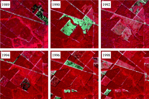
The collection of Landsat images acquired through current and previous Landsat missions (Goward et al. 2006), referred to as the Landsat Record in this article, is a unique data source for reconstructing forest disturbance history for many areas of the globe. Dating back to 1972, this Record makes it possible to document forest changes that have occurred since then, while the fine spatial resolutions of Landsat images provide the spatial details necessary for characterising many of the changes arising from both natural and anthropogenic disturbances (Townshend and Justice 1988). Over the past 30+ years, Landsat images have been widely used in land cover and forest change analysis (Goward and Williams 1997). While the Landsat Record has relatively dense acquisitions in many places of the world, especially in the United States (Goward et al. 2006), largely owing to practical reasons, most previous studies characterised land cover change at relatively sparse temporal intervals (Singh 1989, Lu et al. 2004). Owing to vigorous forest growth in many areas, however, the signal of a forest disturbance may degrade quickly and become spectrally undetectable in just a few years (Figure 1). As a result, some changes likely will not be captured when analysed at sparse temporal intervals (Lunetta et al. 2004). Use of dense image acquisitions is therefore necessary in order to minimise potential omission errors in derived disturbance products.

Figure 1.  Standard false color (i.e., Landsat TM/ETM+ bands 4, 3 and 2 shown as red, green and blue) images showing the spectral progressing of forests recovering from a 1990 stand clearing harvest (the gray areas in the middle of the 1990 image) in a 5.7 km by 5.7 km area near the southern edge of the Lake Moultrie in South Carolina. Immediately after the disturbance, the harvest resulted in drastic spectral changes between the pre- (the 1989 image) and post-disturbance (the 1990 image) images. While the spectral changes were still obvious after two years (the 1992 image), they were difficult to detect after 4-6 years (the 1994 and 1996 images). By 1998, the spectral signature of the disturbed area became visually inseparable from that of the undisturbed forests. This harvest event likely will be missed completely or partially if change analysis is conducted using a pre-1990 image and a post-1992 image.

1.2 The NAFD project

The North American Forest Dynamics (NAFD) project was developed as part of an effort to improve understanding of the carbon budget for North America (Goward et al. 2008). One of the many goals of this project was to evaluate forest disturbance and regrowth history over the last 35+ years for the conterminous U.S. using dense Landsat observations. While a wall-to-wall assessment would be desirable in order to minimise potential sampling errors (Tucker and Townshend 2000), the cost for such an approach would be overwhelming, because data cost was still imposed on Landsat images at the time the NAFD project was conducted. To keep the data cost under control, the NAFD project adopted a sampling approach. Specifically, national estimates of disturbance rates were derived using 23 sample sites selected across the conterminous U.S. (Kennedy et al. 2006). Defined by a path/row tile of the World Reference System (WRS) (Landsat Project Science Office 2000), each sample site had an area of approximately 180 km by 180 km. For each sample site, a Landsat time series stack (LTSS) was developed and used to evaluate forest disturbance history (see Section 2).

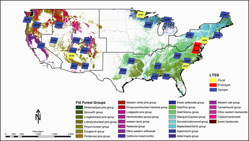
In addition to the 23 sample sites, LTSS were also constructed for three prototype sites and four focal sites through the NAFD and a precursor project. The three prototype sites were developed in the mid-Atlantic region in the 2003 time period to test LTSS procedures prior to full implementation of the NAFD project. By coincidence, one of the prototype sites in Pennsylvania was also selected as a sample site. The four focal (focus on applications) sites were selected to support collaborations between the U.S. Forest Service Forest Inventory and Analysis (FIA) program and the NAFD project, which was intended to facilitate better integration of satellite observations with field measurements collected through the FIA program. Therefore, a total of 29 LTSS have been developed for sites distributed across the conterminous U.S. (Figure 2).

Figure 2.  Distribution of prototype, focal and samples sites where Landsat time series stacks (LTSS) have been assembled through the NAFD project. Each site is represented by a quadrangle. The two numbers separated by a slash in each quadrangle are the WRS path/row number for that site. The background forest group map (Nelson et al. 2007) shows that the majority of the forest groups in the conterminous U.S. have been represented by the study areas covered by the LTSS.

With each LTSS consisting of temporally dense acquisitions, the NAFD project required hundreds of Landsat images. Owing to time and resources constraints, mapping land cover change using such a large number of Landsat images not only required effective change detection algorithms, but also highly automated, high-level preprocessing capabilities to get the images ready for change analysis. This is because standard Landsat imagery products offered by data vendors typically have substantially geometric and radiometric artifacts that often lead to spurious results in land cover change analysis (Townshend et al. 1992). Through the NAFD project, we have developed automated approaches for removing the majority of the radiometric and geometric artifacts contained in standard Landsat imagery products and streamlined the process for producing LTSS that are ready for downstream land cover change analysis. Here we present this process and the developed correction algorithms in detail, along with discussions on some of the characteristics of the LTSS developed through the NAFD project.

Figure 3.  Major steps for developing a Landsat time series stack (LTSS).

Figure 4.  A graphic version of a subset of a full resolution movie loop for the WRS path 16/row 36 LTSS showing the geometric integrity and radiometric consistency among the images of this LTSS. The ground area of each image window is 5.7 km by 5.7 km. Notice the late September and October images appear darker than the pre-mid-September images, illustrating a dependency of the residual spectral variability on the day-of-year of the acquisition date, with which both solar geometry and vegetation phenology vary.

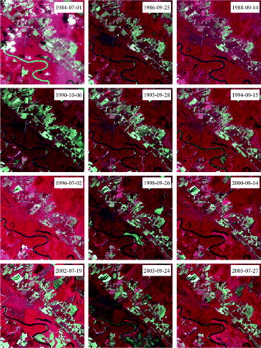
Figure 5.  Same as Figure 4 except that the images were non-IRU (i.e., not corrected using the LEDAPS high level preprocessing algorithms). The displacement of the river running through the lower left quadrant of the image window among the acquisitions shows the magnitude of the geolocation errors in these images while the variable hazy appearances show the impact of changing atmospheric conditions.

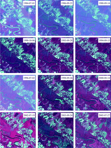
Figure 6.  A comparison of the temporal variability of the top-of-atmospheric (TOA) reflectance and the LEDAPS surface reflectance (SR) for bands 1–3 (a) and bands 4, 5 and 7 (b) for conifer stands within the WRS path 16/row 36 LTSS that did not experience major disturbances. The LEDAPS atmospheric adjustment substantially reduced the temporal variability in the visible bands. The residual temporal variability after the LEDAPS correction appear to be correlated with the day of year of the acquisition date (c and d) or the solar zenith angle (e and f).

2. LTSS definitions

2.1 TM versus MSS Landsat Data

A major goal of the NAFD project was to use the entire Landsat Record (1972–present) to evaluate forest disturbance history. Technically, however, this work was divided into two parts: Thematic Mapper (TM) (1982–present) and multi-spectral scanner (MSS) (1972–1981). This was necessary because the TM and MSS systems used different WRS and the two types of images had different spectral and geometric characteristics (Williams et al. 1984). The MSS part included MSS images acquired by Landsats 1-3. The TM part included TM images acquired by Landsats 4-5 and Enhanced Thematic Mapper Plus (ETM + ) images acquired by Landsat 7. With almost identical spatial and spectral characteristics, TM and ETM+ images are often used interchangeably in land cover change analysis (e.g. Lo and Yang 2002, Vicente-Serrano et al. 2008)

2.2 Landsat time series stack

A Landsat time series stack (LTSS) refers to a sequence of Landsat images acquired at a nominal temporal interval for a particular WRS path/row tile. For the NAFD project, a LTSS typically consisted of one image approximately every two years, which is referred to as biennial LTSS in this paper. Here the selection of the biennial image interval was the compromise between data cost and the necessity to minimise possible omission errors in the derived disturbance products. As discussed earlier (Figure 1), some of the most dramatic manifestations of typical disturbances, such as stand clearing harvesting, may not be detectable at sparse temporal intervals because they can quickly become obscured as successional regrowth takes place. For a small subset of the locations shown in Figure 2, the LTSS consisted of one image per year, which is referred to as annual LTSS hereafter. The annual LTSS were used to evaluate whether there were disturbances that could be detected using annual observations but could not at biennial or longer temporal intervals. Results from this evaluation will be reported separately.

To maintain, as much as possible, a consistent seasonal landscape condition from one year to the next, we constrained seasonal selection to be within the peak green foliage period, which is typically between early June and mid-September for the mid-latitudes and is referred to as the leaf-on season in this paper (to be discussed in more detail in Section 3.1). Unfortunately we also found that for some locations, this limited the availability of nearly cloud-free images within the specified temporal intervals. To adjust for this problem we searched each specified temporal interval and±one year. As will be discussed later, for certain places other approaches will also be needed in order to deal with this problem.

2.3.Imagery ready to use

The main goal of producing a LTSS was to develop imagery time series that could be readily analysed for accurate detection of land cover change and related phenomena, a status called imagery-ready-to-use (IRU) (Goward 2006). Here the IRU of a LTSS is defined in two aspects:

a.

First, it should consist of highest quality images to the extent allowed by data availability, where quality is defined as having minimum engineering problems and minimum cloud and shadow contamination.

b.

Second, the images in each LTSS should have the highest achievable geometric and radiometric integrity: - Subpixel corregistration accuracy among the involved images is critical in order to minimise spurious changes arising from misregistration errors (Townshend et al. 1992). - High radiometric integrity, which is achieved through accurate calibration and adjustment to surface reflectance, permits more reliable characterisation of land cover and land cover change (e.g. Song et al. 2001, Song et al. 2002).

It should be noted that great efforts have been given to produce IRU quality products using images acquired by coarser spatial resolution instruments such as the advanced very high resolution radiometer (AVHRR) and the moderate resolution imaging spectroradiometer (MODIS) (e.g. Vermote et al. 2002, Wolfe et al. 2002, Ouaidrari et al. 2003, Tucker et al. 2005). Standard Landsat imagery products, however, typically have not been subjected to such a high level of geometric and radiometric integrity. This occurs, in part, because of the large effort normally required to process individual images in order to achieve such a high quality level.

3. LTSS development

In order to develop the LTSS required by the NAFD project at affordable effort levels, we automated the high level preprocessing algorithms required to produce IRU quality Landsat images and streamlined the entire process for generating LTSS using standard imagery products offered by most Landsat data vendors. This process comprised an image selection protocol, automated high level preprocessing algorithms and IRU quality verification procedures (Figure 3). The high-level preprocessing algorithms included updated radiometric calibration for Landsat 5 images, atmospheric adjustment to surface reflectance, precision registration and orthorectification. Here the term ‘high level’ is used to differentiate these algorithms from the standard correction algorithms for Landsat images (Landsat Project Science Office 2000). These high level preprocessing algorithms were implemented as fully automated routines in the Landsat Ecosystem Disturbance Adaptive Processing System (LEDAPS) to facilitate batch job processing. The LEDAPS was an adaptation of the MODIS MODAPS system (Justice et al. 2002) for processing Landsat data. It allowed rapid generation of higher-level products from raw Landsat radiometry using the correction algorithms described in this paper (Masek et al. 2006).

3.1 Image selection

The main purpose for image selection was to identify high quality Landsat acquisitions needed to constitute a LTSS. While the actual temporal intervals between consecutive acquisitions within a LTSS could vary owing to data availability, the goal was to select one image within every two years for a biennial LTSS and one image every year for an annual LTSS. Two issues were considered in selecting a high quality image:

a.

First, a selected image must be acquired during the leaf-on season. Images acquired outside this temporal window are generally not suitable for forest change analysis, because leaf-off deciduous forests can be spectrally confused with disturbed forest land. Based on phenology studies using MODIS and AVHRR measurements (Schwartz et al. 2002, Zhang et al. 2003), the leaf-on season included the months between June and mid-September for most areas in the conterminous U.S.; but this criterion was relaxed to include May and October in southern U.S.

b.

Second, in order to maximise the proportion of usable pixels within each selected image, it should have minimum or no quality problems arising from instrument errors or from cloud and shadow contamination.

Although the data searching systems developed by the U.S. Geological Survey (USGS) provided a quality index and a cloud cover index, we were unable to automate the selection of desirable images using these indices because an initial analysis revealed that these indices were not always reliable. Instead, we visually inspected the browse images using the USGS Global Visualization Viewer (GloVis) system (http://glovis.usgs.gov/) to determine the best quality images. For each selected image, a cloud cover was estimated based on visual inspection of the browse image.

Most selected images were purchased from the USGS National Center for EROS. The specifications for these images included 28.5 m pixel size, cubic convolution resampling and UTM projection. To reduce data cost, we incorporated some publically available Landsat data sets in developing the NAFD LTSS. We discovered that the USGS, in cooperation with the U.S. Forest Service under the project Monitoring Trends in Burn Severity (MTBS), was producing Landsat data sets similar to the NAFD LTSS for locations where major wild land fires had occurred. These data sets were freely available for use by interested researchers and some of them were used in the NAFD project. The main difference between the two data sets was that the MTBS used the Albers Conical Equal Area projection rather than the UTM projection used in the NAFD project. Therefore, the MTBS images selected for use in the NAFD project were reprojected using the NAFD specifications. In addition, suitable images in the GeoCover data sets acquired through NASA's Science Data Buy program (Tucker et al. 2004) were also included in developing the NAFD LTSS.

3.2 Updated radiometric calibration

Radiometric calibration is part of the USGS process for producing standard level 1 Landsat imagery (Landsat Project Science Office 2000). For Landsat 7 images, the ETM+ sensor has been carefully monitored since launch (Markham et al. 2004). As such, the conversion of ETM+ Level 1 radiometry to at-sensor radiance was a simple matter of applying the rescaling gains and biases from the ETM+ header file to the imagery. For Landsat 5 images, however, there have been many revisions to the calibration coefficients (Markham and Barker 1986, Chander and Markham 2003, Chander et al. 2004, Markham et al. 2004):

1.	Prior to May 2003–internal calibration (IC) lamps measurements were used to determine the gain coefficient. During the 1990s it became increasingly apparent that variations in the IC-derived gain values reflected a combination of real changes in sensor calibration (i.e. detector sensitivity and filter properties) and changes in the IC lamps themselves.
2.	May 2003 to April 2007–following the Landsat-7/Landsat-5 under-fly experiment in April 1999, a cross-calibration between ETM+ and TM was established (Chander et al. 2004, Teillet et al. 2004), which was used to determine the gain value for Landsat 5 images.
3.	After April 2007–further investigations using invariant ground targets in North Africa suggested that the initial lookup table was in error for the first part of the Landsat-5 history (about 1985–1992). Instead, records of at-sensor radiance from these sites suggested a more gradual decay in gain throughout the mission life. As such, Landst-5 imagery processed after April 2007 used a revised lookup table (Chander et al. 2004).

Within LEDAPS, the production date of a Landsat-5 image was used to determine which calibration was originally applied to the image. As appropriate, the original calibration was ‘undone’ by applying the reciprocal of the gain and the most recent (the post April 2007 version) lookup table was applied. Conversion to top-of-atmosphere reflectance was then performed for the reflective bands using the scene-specific solar geometry and sensor-specific band-passes convolved with the CHKUR exo-atmospheric irradiances from MODTRAN-4 (Markham and Barker 1986, Landsat Project Science Office 2000).

The calibration of the Landsat 5 thermal band was not monitored for most of the history of the Landsat 5. While a radiance correction to the calibration was published in late 2007 (Barsi et al. 2007), all the LTSS had already been produced by that time. Therefore, for this band, raw DN was converted to top-of-atmosphere (apparent) temperature using the standard approach provided by Markham and Barker (1986) for TM images and by the Landsat Project Science Office (2000) for ETM+ images.

3.3 Atmospheric adjustment to surface reflectance

The LEDAPS atmospheric adjustment algorithm was designed to calculate surface reflectance by compensating for atmospheric scattering and absorption effects on the TOA reflectance (Masek et al. 2006). The basic assumptions of this algorithm include:

a.	The target is Lambertian and infinite; and
b.	The gaseous absorption and particle scattering in the atmosphere can be decoupled.

This approach, based on a similar method used for MODIS and AVHRR (Vermote et al. 2002), uses the 6S radiative transfer code to compute the transmission, intrinsic reflectance and spherical albedo for relevant atmospheric constituents (Vermote et al. 1997).

The relevant atmospheric constituents include gases, ozone, water vapor and aerosols. Ozone concentration was derived from the total ozone mapping spectrometer (TOMS) aboard the Nimbus-7, Meteor-3 and Earth Probe platforms as well as from NOAA's Tiros Operational Vertical Sounder (TOVS) ozone data when TOMS data were not available. Column water vapour was taken from NOAA National Centers for Environmental Prediction (NCEP) re-analysis data (available at http://dss.ucar.edu/datasets/ds090.0/). Digital topography (1km GTopo30) and NCEP surface pressure data were used to adjust Rayleigh scattering to local conditions. Aerosol optical thickness (AOT) was directly derived from the Landsat image using the dark, dense vegetation method of Kaufman et al. (1997).

This LEDAPS atmospheric adjustment approach has previously been used to correct the GeoCover Landsat images to produce 1990 and 2000 surface reflectance data sets for North America. Comparisons of the LEDAPS surface reflectance products with ground-based optical thickness measurements and simultaneously-acquired MODIS imagery indicated comparable uncertainty in Landsat surface reflectance as compared with the standard MODIS reflectance product (Masek et al. 2006).

3.4 Precision registration and ortho-rectification

Raw satellite images usually contain significant geometric distortions arising from a range of sources, including platform and instrument related sources, as well as those due to the Earth's curvature, rotation and topography (Toutin 2003). While some of the distortions have been removed through the standard level 1G (L1G) systematic correction, substantial geolocation errors still exist in many L1G images. An assessment of USGS L1G images acquired for the NAFD project revealed that these standard image products, especially the Landsat 5 images, could be mis-registered from one acquisition date to another by as much as 500 m. This resulted primarily from uncontrolled orbital drift. Further analysis of image relief displacement as a result of topography has shown that at swath edges geolocation is in error by about 120 m per kilometer of elevation. The LEDAPS precision registration and orthorectification algorithms were designed to reduce the geolocation errors to subpixel levels.

3.4.1 Precision registration

A prerequisite for performing orthorectification is that the orbit of each image acquisition is known precisely. The LEDAPS orthorectification algorithm uses nadir view pixels to calculate satellite orbit. The purpose of precision registration is to calculate the geolocation of nadir view pixels accurately to allow precise determination of satellite orbit. This routine uses an automatic tie-point searching algorithm to register a target image to an orthorectified base image. In the LEDAPS system the global GeoCover 2000 images were used as the based images for precision registration. The GeoCover data set consists of orthorectified Landsat images with average geolocation errors of 50 m or less for all land areas of the globe (Tucker et al. 2004).

Ideal tie points for image registration include edges or corners of ground features that remained relatively stable, both geometrically and radiometrically, between the target image and the base image. Road intersections, bridges and dams are examples of good tie points. For a point in the target image, its tie point in the base image is determined in the following steps.

1.	Calculate the projected location of that point in the base image based on the original coordinates of both the base image and the target image.
2.	Calculate the correlation coefficient (r) between the base image and the target image using a local window centred at each point.
3.	Move the local window in the base image within a predefined searching window around the projected location as determined in step 1 and recalculate r.
4.	If the maximum r value is higher than a predefined threshold value for r (r-threshold) and the number of r values higher than r-threshold is less than a predefined threshold value (N-threshold), the center of the local window in the base image that gives the highest r value is the tie point. Otherwise, no tie point is found for that particular point in the target image. Here the N-threshold is used to constrain tie points to object edges or corners. Based on experiments with a large number of images, we selected 0.6 for the r-threshold and 3 for the N-threshold.

Most of the points identified this way should be good tie points, but some could be spurious. False tie points are identified and removed as follows.

1.	Calculate the average offset of the target image from the base image using the tie points.
2.	Assuming the target image would be shifted using the calculated offset, calculate the residual geolocation error of the shifted image at each tie point.
3.	Find the point with the maximum residual error. If the error is more than a predefined threshold (e.g., half a pixel), discard that point and repeat steps 1–3. Otherwise screening of the tie points is complete.

A successful precision registration requires a minimum number of predefined tie points (e.g., 10) after the screening. For the combined precision registration and orthorectification process, only successfully registered images are further processed using the orthorectification algorithm described in Section 3.4.2.

During processing of the NAFD images, we noticed that in extreme cases the geolocation errors in the standard L1G TM images could be more than 10 km, or 300 TM pixels, in one dimension. The speed of the searching algorithm described above deteriorated greatly when the searching window was larger than 300 by 300 TM pixels. To alleviate this problem, a preliminary registration was performed to remove the gross geolocation error in the target image before performing the precision registration at the full resolution. The preliminary registration consisted of the same steps as described above but those steps were performed on a coarser resolution version of the target image and the base image derived through spatial aggregation. With search windows of up to ±50 pixels, this two-step approach can allow successful identification of tie points even when two images are offset by as much as 60 km.

3.4.2 Orthorectification

For each precision registered image, the nadir pixels define the instantaneous orbit of the platform when the target image was acquired. Through orthorectification the relief displacement of each pixel is calculated using satellite altitude, an Earth model, terrain height and the pixel's location in the precision registered image. Equations for orthorectification have been provided in the Landsat 7 Image Assessment System (IAS) Geometric Algorithm Theoretical Basis Document (available at http://ldcm.nasa.gov/library/L7_IAS_070998.pdf). In the LEDAPS system, terrain height was obtained from the digital elevation model (DEM) data set produced through the Shuttle Radar Topography Mission (SRTM) (Rabus et al. 2003). This data set is available at the 30 m spatial resolution for the U.S. and at the 90 m resolution for the rest of the world.

To ensure that subpixel co-registration accuracy is achieved, following orthorectification each image is checked against the appropriate base image using the tie points identified during the precision registration process. If a residual error higher than a predefined criteria is found (e.g., half a pixel), a polynomial transformation is then performed to remove possible skew or rotation errors in the target image. In our tests, we found that first or second order polynomial transformations were necessary for some early Landsat images.

It should be noted that although the above described precision registration and orthorectification routines comprise multiple steps – to minimise the impact of resampling on the integrity of image geometry and radiometry (Khan et al. 1995, Lillesand et al. 2004) – the two routines were implemented such that each input image would not be resampled more than once when processed using the LEDAPS.

3.5 LTSS IRU quality verification

Prior to its use in downstream applications, each developed LTSS was verified to determine whether the processed images had geometric or radiometric artefacts. Artefacts in the LTSS can result from:

a.	unidentified quality problems with the input images;
b.	unknown bugs that may exist in the LEDAPS pre-processing algorithms;
c.	incorrect inputs regarding the geometry or radiometry of the concerned images.

Identified artefacts that were attributed to the LEDAPS processing were removed or minimised either by supplying appropriate inputs to the algorithms or by fixing the identified bugs. For issues that were attributed to quality problems in the input images, those images were either replaced with images that met the image selection criteria described in Section 3.1, or dropped if no qualified image was available.

The verification procedures included a quick visualisation approach and a spectral-temporal profile method. Prior to the verification, the images of each LTSS were clipped such that they had exactly the same spatial domain.

3.5.1 Image clipping

As noted earlier, due to difficulties in orbital control, satellite orbits can shift slightly among repeat passes. As a result, several images for a single WRS location are not necessarily congruent to the same geographic region (i.e. they do not overlay on top of each other exactly). Therefore, pixels near the edge of a WRS tile can have valid values on some dates but not on other dates. Temporal analysis of such incomplete observations is difficult. To avoid this problem, a common area mask was used to exclude such observations from being analysed. For each LTSS, this mask was defined as the maximal geographic area where all image acquisitions in that LTSS had valid pixel values (except the missing data area caused by missing scan lines that may exist in certain acquisitions) and all images of that LTSS were clipped using this mask.

3.5.2 Visual verification

Visual inspection is a simple yet effective method for verifying the quality of the LTSS images. By flipping the images from one date to another, an experienced image analyst can quickly identify inconsistencies among the images, which are often indicators of geometric or radiometric artefacts, and can gain first hand knowledge of the change processes to be analysed later. To facilitate quick visualisation of the LTSS images, the clipped images were converted to the JPEG format (note: other visualisation ready formats can be used in the place of the JPEG format here), which were then assembled to create a movie loop. For each LTSS a single stretching method was used during the conversion in order to create comparable colour tones among the images. After testing with different stretching methods, we found that, except in semiarid areas where vegetation cover is relatively low and the background is bright, a single stretching method per band could be applied to all the images. The general linear stretching equation is:

1

where in_value and out_value are the input surface reflectance (%) and output stretched values respectively. The single set of refl_min and refl_max applicable to most vegetated areas are given in Table 1.

Table 1. Parameters used in Equation (1) for stretching the surface reflectance images to create JPEG images for use in the movie loop. Only standard false colour images were created using the TM/ETM+ bands 4, 3 and 2 shown in red, green and blue colours.

	Refl_min (%)	Refl_max (%)
Band 2	0	15
Band 3	0	15
Band 4	2	50

In the semiarid western U.S., some partially vegetated areas appeared saturated in bands 2 and 3 when stretched using Equation (1). To avoid this problem, the following nonlinear stretching method was applied to those two bands for images in this area (band 4 was stretched using Equation (1));

2

For each LTSS one movie loop was created to show the entire LTSS at a browse resolution (i.e. 285 m). The browse resolution images were generated by subsampling the full resolution images using a 10:1 ratio in both along- and cross-track directions. In addition, three movie loops were created at the full 28.5 m resolution for 15 km by 15 km image windows randomly selected from within each LTSS. The browse level movie loop provided an overview of the radiometric integrity of all images within a LTSS, while the full resolution movie loops allowed more detailed inspection of both the geometry and radiometry of the images in each LTSS.

3.5.3 Spectral-temporal profile

In order to provide a more quantitative assessment of the radiometric consistency among the images within each LTSS, we also evaluated the temporal variability of the spectral values of targets that were considered relatively stable over time. As the primary use of the LTSS assembled in this study was forest change analysis, the ‘stable targets’ in this context referred to conifer stands that did not have visual signs of being disturbed during the entire observing period of each LTSS. For each LTSS, a few examples of such stands were identified and the average spectral values of those stands were calculated for each acquisition date. The values for all dates were then plotted as a function of acquisition date.

4. Example results and discussions

The LTSS development procedures were used to produce the LTSS for the TM part for the 29 locations shown in Figure 2. Each LTSS was verified using the above described verification procedures. Verification results revealed high levels of geometric integrity and radiometric consistency among the images of each LTSS, which can be illustrated using example verification results for a typical LTSS.

Figure 4 shows a graphic version of a subset of a full resolution movie loop created using the LTSS for the sample location WRS path 16/row 36. To illustrate the effectiveness of the geometric and radiometric correction algorithms implemented in the LEDAPS system, a movie loop was created for the same area using non-IRU images (i.e., without performing the LEDAPS algorithms for precision registration, orthorectification and atmospheric adjustment) (Figure 5). Displacement of the river running through the lower left quadrant of the image from one acquisition date to another shows the magnitude of the geolocation errors in the non-IRU images. After the LEDAPS precision registration and orthorectification, the river is consistently found in the same location in different dates (Figure 4), indicating that the majority of the geolocation errors were removed through the LEDAPS corrections. The variable hazy appearances of the non-IRU images show the impact of changing atmospheric conditions on those images (Figure 5), much of which was removed after the LEDAPS atmospheric adjustment (Figure 4).

A quantitative illustration of the effectiveness of the LEDAPS atmospheric adjustment algorithm is provided in the spectral-temporal plots created using ‘stable’ conifer stands. As discussed earlier, ‘undisturbed’ conifer forests should have relatively stable spectral values from one year to another during the peak-growing season. The top-of-atmospheric (TOA) reflectance values for the selected ‘stable’ stands, however, varied from 8.9% to 12.9% in band 1 (blue band), 6.8% to 9.6% in band 2 (green band) and and 4.5% to 6.7% in band 3 (red band) (Figure 6(a)). After the LEDAPS processing, the conifer stands had much narrower spectral variations from one year to another (Figure 6(a)). The temporal variability of the spectral values of the selected conifer stands as measured by the 22-year standard deviation was reduced by 78%, 55% and 44% for bands 1, 2 and 3 respectively (Table 2). The calculated surface reflectance (SR) values were much closer to those derived from MODIS measurements than the TOA reflectance (Table 2, see also Masek et al. 2006).

Table 2. 22-year (1984–2005) mean and standard deviation of the spectral value of “stable” conifer stands selected from the WRS path 16/row 36 LTSS.

	Surface reflectance (%)		TOA reflectance (%)
	Mean	Standard deviation	Mean	Standard deviation
Band 1	2.02	0.31	10.39	1.39
Band 2	3.62	0.48	7.93	1.06
Band 3	2.22	0.47	5.39	0.84
Band 4	26.97	3.09	23.42	2.10
Band 5	11.35	1.48	9.96	1.51
Band 7	4.43	0.90	3.84	0.77

Because the atmospheric effect in the infrared bands (bands 4, 5 and 7) is predominantly a transmission effect (Vermote et al. 2002), the spectral value of the conifer stands increased slightly when it was converted from TOA reflectance to surface reflectance by the LEDAPS atmospheric adjustment algorithm (Figure 6(b)), which also resulted in a slight change in the 22-year standard deviation (Table 2).

The residual temporal variability of the surface reflectance values appeared to be correlated with the day-of-year (DOY) calculated from the acquisition date (Figure 6(c) and (d)), or with the solar zenith angle at the acquisition of the Landsat images (Figure 6(e) and (f)). This means that a good portion of the residual temporal variability likely can be explained by actual variations in either solar geometry or vegetation phenology, or both.

The fact that the LEDAPS atmospheric adjustment algorithm greatly reduced the temporal variability of stable targets in the visible bands but had much less impact on the infrared bands may suggest that such adjustment is less critical for downstream applications that only rely on the infrared bands or use spectral indices such as the normalised difference moisture index (NDMI) that are calculated by only using the infrared bands. However, most vegetation studies using remote sensing images likely will benefit from atmospheric adjustment because many spectral vegetation indices are essentially calculated by contrasting the visible and infrared bands in different ways (e.g. Qi et al. 1994, Jurgens 1997). In addition, use of visible bands or combined use of visible and infrared bands have been found more effective in land cover change analysis than using just the infrared bands alone (e.g. Ridd and Liu 1998, Wilson and Sader 2002, Zhan et al. 2002).

5. Summary and implications

The Landsat record provides a unique opportunity for understanding the dynamics of land cover and related surface properties for the decades dating back to the early 1970s. While Landsat images have been used in numerous applications, not many studies systematically explored the rich temporal information by using dense Landsat observations, which is needed in order to minimise change detection omission errors that may exist in change products derived using sparse acquisitions. This may be attributed to many practical reasons, including data availability issues and a lack of capabilities for producing large quantities of IRU quality images.

The LTSS concept developed in this study and the streamlined process make it possible to produce dense time series of IRU quality Landsat observations for land cover change and other downstream analyses at affordable effort levels. The automated high level preprocessing algorithms implemented in the LEDAPS system provide the technical capabilities for rapidly producing large quantities of IRU quality LTSS. The verification procedure is necessary to ensure the IRU quality of the produced LTSS. In fact, during the production of the LTSS for the NAFD project, the verification procedures revealed a number of problems with earlier versions of the LEDAPS algorithms, which were fixed following the discovery of those problems.

With the mass processing capacity provided by the LEDAPS system, the ability to assemble LTSS for any particular area will depend on the availability of Landsat acquisitions within the specified temporal intervals for that area. The temporal richness of historical Landsat archives has been shaped by many factors, including instrument capabilities, data acquisition, pricing and distribution policies, as well as changes in the management responsibility of the Landsat program (Draeger et al. 1997, Green 2006). An in-depth analysis of the USGS Landsat archive by Goward et al. (2006) revealed that the conterminous U.S. had the best spatial and temporal coverage of Landsat acquisitions, with the caveat that little was known on the Landsat data holdings at international ground receiving stations at the time of that study. Even within the conterminous U.S., however, cloud free images were difficult to find during the peak growing season of certain target years for places characterised by constant cloudy conditions. In the western Pennsylvania site (WRS path 17/row 31), for example, even the least cloudy images had 10%, 40% and 15% cloud cover during the growing season of 1988, 1990 and 1992, respectively. For the NAFD project, we had difficulties to find cloud-free images for certain target years for many places in eastern U.S. that satisfied the image selection protocol described in Section 3.1. As a result, many of the LTSS consisted of at least one image that had more than 5% cloud cover (Table 3) and there were more images having significant though less than 5% cloud cover.

Table 3. Number of images that had at least 5% cloud cover in the developed LTSS in eastern U.S.

WRS2 path/row	Location	Total number of images	Number of images having at least 5% cloud cover
12/27	Northern Maine	13	5
12/31	Massachusetts	13	2
14/32	Delaware	13	4
15/33	Maryland/Washington DC	12	3
15/34	Virginia	22^1	6
16/36	Southern North Carolina	13	1
16/37	South Carolina	13	3
17/31	Western Pennsylvania	26^2	20
18/35	Western North Carolina	13	4
19/39	Western Florida	12	1
21/37	Central eastern Mississippi	12	0
21/39	Southern Mississippi	12	3
22/28	Northern Michigan	12	2
26/36	Oklahoma	12	1
27/27	Northern Minnesota	13	6
27/38	Eastern Taxes	12	1
Notes: ^1This is an annual LTSS, i.e., it consists of one image per year;
^2This site was so cloudy that for many of the target years we could not find a cloud free image during the leaf-on season. For each of those years, at least two partially cloudy images were acquired in order to create a composite with minimum or no cloud contamination.

It should be noted that even a small percentage of cloud cover in an image (e.g. 1%) can result in significant errors in a derived forest change product if the clouds are not flagged properly. An unflagged cloud over a forest is likely to be mapped as a forest change. If all clouds in an image are over forests and are not flagged properly, 1% cloud cover can result in 1% or more false detection of change pixels in that image. According to Masek et al. (2008), most areas in North America have annual disturbance rates less than 1%, with the highest annual disturbance rates being 2%-3% in southeastern U.S. Therefore, even 1% cloud cover in an image could result in false changes that may be equivalent to or more than the amount of actual changes. A change detection algorithm has to be able to flag the cloudy pixels properly in order to avoid them being mapped as change.

Another way to reduce false changes arising from cloud contamination in constantly cloudy areas is to create a cloud-free image mosaic using partially cloudy acquisitions through cloud clearing compositing. We have noticed through the NAFD project that for many of the target years where we could not find cloud-free images, multiple partially cloudy images did exist during the peak growing season of the concerned years. Compositing has been widely used with coarse spatial resolution satellite data sets as a technique to minimise the impact of cloud contamination and different techniques have been developed for use with those data sets (e.g. Holben 1986, Huete et al. 2002). However, those techniques likely will not be directly applicable to images acquired by a single Landsat or Landsat-class instruments. Because such instruments have nominal revisiting cycles of about two weeks or longer, each of them can only collect a few acquisitions for a given location during the growing season of a particular year and some of the acquisitions can be months apart. Therefore, a cloud clearing compositing algorithm for use with such a few number of images will not only need to identify and replace the pixels contaminated by cloud and shadow, but also to make appropriate adjustment to the phenological differences among the concerned images (e.g. Helmer and Ruefenacht 2005). For producing the large quantities of Landsat images needed to assemble annual or biennial LTSS, such an algorithm has to be automated and integrated into a streamlined process like the one described here.

An inventory of Landsat holdings at international ground receiving stations will be needed in order to determine the feasibility to assemble LTSS at a specific temporal interval for regions outside the U.S. According to the Goward et al. (2006) study, use of the USGS archive alone will not allow construction of LTSS at 5-year or shorter temporal intervals for the entire Landsat history for many regions outside the U.S. For regions where existing Landsat acquisitions available at the USGS and international archives are inadequate for assembling time series of satellite observations, use of data fusion techniques to harness images acquired by other Landsat-class instruments may allow construction of such time series of observations for a portion of the land remote sensing history.

Notes on contributors

Chengquan Huang is a Research Faculty in the Geography Department of the University of Maryland. He received his B.S. and M.S. from Peking University and Ph.D from the University of Maryland. His research interests include characterisation and monitoring of land cover, biomass and ecosystem dynamics by integrating satellite and non-satellite observations. Dr Huang is currently engaged in multiple projects designed to gain understanding of regional and global scale forest dynamics using fine resolution satellite data sets and is developing automated image pre-processing and land cover change analysis algorithms for achieving the goals of those projects.

Dr Goward is Professor of Geography at the University of Maryland. He serves on the editorial board of Remote Sensing of Environment and has been involved in land remote sensing since the early 1970s. Recently his work has focused on automated processing and analysis of regional and global data sets from Landsat, AVHRR and MODIS. From 1997 to 2002 he served as the Team Leader for the NASA Landsat Science Team and is currently a member of the USGS/NASA Landsat Science Team. He co-chaired the 2^nd and 3^rd FACA advisory committees for the USGS National Land Satellite Remote Sensing Data Archive advisory committee. He was awarded the USGS John Wesley Powell Award in 2006 and the USGS/NASA William T. Pecora Award in 2008 for contributions to the Landsat Mission.

Dr Masek is a Research Scientist in the Biospheric Sciences Branch at NASA Goddard Space Flight Center. His research interests include mapping land-cover change in temperate environments, carbon cycle science, application of advanced computing to remote sensing and satellite remote sensing techniques. As Deputy Project Scientist for the Landsat Data Continuity Mission (LDCM), he has focused on advancing the development of new scientific products for the LDCM mission. He received a B.A. in Geology from Haverford College and a Ph.D in Geological Sciences from Cornell University.

Dr Gao is a research scientist with Earth Resources Technology (ERT), Inc., a contractor at NASA Goddard Space Flight Center. He was a research associate professor with the Department of Geography, Boston University from 1998 to 2004. He received the B.A. degree in geology and the M.S. degree in remote sensing from Zhejiang University, Hangzhou, China, in 1989 and 1992, respectively, the Ph.D. degree in geography from Beijing Normal University, Beijing, China, in 1997 and the M.S. degree in computer science from Boston University, Boston, MA, in 2003. He is a member of the Landsat science team since September 2006. His recent research interests include remote sensing modeling, multi-sensor data fusion and applications.

Eric Vermote received the Ph.D. degree in atmospheric optics from the University of Lille, Lille, France, in 1990. He is currently a Senior Research Scientist with the Department of Geography, University of Maryland at College Park. He is a member of the Moderate Resolution Imaging Spectroradiometer Science Team, the NASA National Polar-orbiting Operational Environmental Satellite System Preparatory Project Science Team and the Landsat Data Continuity Mission Science Team and is responsible for the atmospheric correction over land surfaces in the visible-to-middle infrared spectral range. His research interests cover radiative transfer modelling, vicarious calibration, atmospheric correction and aerosol retrieval.

Nancy Thomas is with the Department of Geography at the University of Maryland and works as Project Manager for the North American Forest Dynamics study. She received a B.A. in Geography from San Francisco State University and a M.A. from the University of Maryland. Ms. Thomas worked as Remote Sensing Analyst and Coordinator for Pacific Meridian Resources/Space Imaging in Emeryville, California, where she designed and managed remote sensing and GIS projects which focused on land cover change detection, object-oriented image classification and detailed vegetation mapping with high-resolution imagery. Her current research focus is on validation techniques for Landsat time series disturbance maps and on integrating USFS Forest Inventory Analysis (FIA) plot data with remotely sensed imagery.

Karen Schleeweis received a Masters degree in Geography from the University of Maryland, College Park, in 2005. She is currently working on a Ph.D in Geography with the University of Maryland and is a graduate research assistant for the North American Forest Dynamics (NAFD) project. Her research interests cover landscape ecology, biogeography, remote sensing for ecosystem monitoring, forest disturbance and carbon management.

Dr Robert Kennedy is a research associate in the Department of Forest Ecosystems and Society at Oregon State University. His research focuses on issues related to understanding ecological systems at broad spatial scales, including sampling, modelling and remote sensing.

Dr Zhu works for the U.S. Geological Survey as the bureau's fire science lead. He is responsible for setting research priorities and directions, enhancing collaborations and science support for the Department of the Interior and the USDA Forest Service and coordinating and representing fire research activities across all of the USGS disciplines. Prior to his current responsibility, Dr. Zhu was a research scientist at USGS working on wild land fire and fuel mapping. He was the USGS principal investigator for the LANDFIRE project. He also worked for Forest Service in the early 1990s and briefly in 2008. Dr. Zhu has a B.S. in forestry from Nanjing Forestry University, China and MS and PhD in remote sensing and forestry from University of Michigan.

Dr Eidenshink is a Physical Scientist at the USGS Earth Resources Observation and Science (EROS) Center. He has been involved in remote sensing and GIS research for over 30 years and has worked in the research and development of environmental data sets from satellite observations and application of remote sensing technology in fire science. He has served as the leader of the Fire Science at EROS, which includes LANDFIRE, Monitoring Trends in Burn Severity, fire danger monitoring and other fire science researches. He is currently Deputy Director of USGS EROS.

Dr Townshend is a Professor and Chair of Geography at the University of Maryland. He received the B.S. and Ph.D. degree in geography from the University College London. His research interests are in land-cover change, remote sensing and environmental information systems. He is a member of NASA's MODIS Science Team and Principal Investigator of the Global Land Cover Facility. He was Chair of GOFC-GOLD from 2000 to 2006 and co-chair of the IGOS-P's Land Theme from 2004 to present. He serves as chair of the UNEP's Division of Environmental Information, Assessment and Early Warning for North America. In 2007, he was the Terrestrial Lead for the CEOS Response Team to the GCOS Implementation Plan. From 1995 to 1998, he was Chairman of the Joint Scientific and Technical Committee of GCOS.

References

- Band , L.E. 1993 . Effect of land surface representation on forest water and carbon budgets . Journal of Hydrology , 150 : 749 – 772 .
- Barsi , J.A. , Hook , S.J. , Schott , J.R. , Raqueno , N.G. and Markham , B.L. 2007 . Landsat-5 Thematic Mapper Thermal Band Calibration Update . IEEE Geoscience and Remote Sensing Letters , 4 ( 4 ) : 552 – 555 .
- Chander , G. , Helder , D.L. , Markham , B.L. , Dewald , J.D. , Kaita , E. , Thome , K.J. , Micijevic , E. and Ruggles , T.A. 2004 . Landsat-5 TM reflective-band absolute radiometric calibration . IEEE Transactions on Geoscience and Remote Sensing , 42 ( 12 ) : 2747 – 2760 .
- Chander , G. and Markham , B. 2003 . Revised Landsat-5 TM Radiometric Calibration Procedures and Postcalibration Dynamic Ranges . IEEE Transactions on Geoscience and Remote Sensing , 41 ( 11 ) : 2674 – 2677 .
- DeFries , R. , Hansen , A. , Newton , A.C. and Hansen , M.C. 2005 . Increasing isolation of protected areas in tropical forests over the past twenty years . Ecological Applications , 15 ( 1 ) : 19 – 26 .
- Draeger , W.C. , Holm , T.M. , Lauer , D.T. and Thompson , R.J. 1997 . The availability of Landsat data: past, present and future . Photogrammetric Engineering & Remote Sensing , 63 ( 7 ) : 869 – 876 .
- Giambelluca , T.W. , Nullet , M.A. , Ziegler , A.D. and Tran , L. 2000 . Latent and sensible energy flux over deforested land surfaces in the eastern Amazon and northern Thailand . Singapore Journal of Tropical Geography , 21 ( 2 ) : 107 – 130 .
- Goward , S. , Irons , J. , Franks , S. , Arvidson , T. , Williams , D. and Faundeen , J. 2006 . Historical record of landsat global coverage: Mission operations, NSLRSDA and international cooperator stations . Photogrammetric Engineering and Remote Sensing , 72 ( 10 ) : 1155 – 1169 .
- Goward , S.N. , 2006 . Future of land remote sensing: What is needed . In Joint Agency Commercial Imagery Evaluation (JACIE) Workshop , Patuxent National Wildlife Research Center , Laurel , MD , March 14–16 , 2006 .
- Goward , S.N. , Masek , J.G. , Cohen , W. , Moisen , G. , Collatz , G.J. , Healey , S. , Houghton , R. , Huang , C. , Kennedy , R. , Law , B. , Turner , D. , Powell , S. and Wulder , M. 2008 . Forest Disturbance and North American Carbon Flux . EOS Transactions, American Geophysical Union , 89 ( 11 ) : 105 – 106 .
- Goward , S.N. and Williams , D.L. 1997 . Landsat and earth systems science: develoment of terrestrial monitoring . Photogrammetric Engineering and Remote Sensing , 63 ( 7 ) : 887 – 900 .
- Green , K. 2006 . Landsat in Context: The Land Remote Sensing Business Model . Photogrammetric Engineering and Remote Sensing , 72 ( 10 ) : 1147 – 1155 .
- Helmer , E.H. and Ruefenacht , B. 2005 . Cloud-free satellite image mosaics with regression trees and histogram matching . Photogrammetric Engineering and Remote Sensing , 71 ( 9 ) : 1079 – 1089 .
- Hirsch , A.I. , Little , W.S. , Houghton , R.A. , Scott , N.A. and White , J.D. 2004 . The net carbon flux due to deforestation and forest re-growth in the Brazilian Amazon: analysis using a process-based model . Global Change Biology , 10 ( 5 ) : 908 – 924 .
- Holben , B.N. 1986 . Characteristics of maximum-value composite images from temporal AVHRR data . International Journal of Remote Sensing , 7 ( 11 ) : 1417 – 1434 .
- Houghton , R.A. 2003 . Why are estimates of the terrestrial carbon balance so different? . Global Change Biology , 9 ( 4 ) : 500 – 509 .
- Huete , A. , Didan , K. , Miura , T. , Rodriguez , E.P. , Gao , X. and Ferreira , L.G. 2002 . Overview of the radiometric and biophysical performance of the MODIS vegetation indices . Remote Sensing of Environment , 83 ( 1–2 ) : 195 – 213 .
- Jurgens , C. 1997 . The modified normalized difference vegetation index (mNDVI) – a new index to determine frost demages in agriculture based on Landsat TM data . International Journal of Remote Sensing , 18 ( 17 ) : 3581 – 3594 .
- Justice , C.O. , Townshend , J.R.G. , Vermote , E.F. , Masuoka , E. , Wolfe , R.E. , Saleous , N. , Roy , D.P. and Morisette , J.T. 2002 . An overview of MODIS Land data processing and product status . Remote Sensing of Environment , 83 ( 1–2 ) : 3 – 15 .
- Kaufman , Y.J. , Wald , A.E. , Remer , L.A. , Gao , B.-C. , Li , R.-R. and Flynn , L. 1997 . The MODIS 2.1 mm Channel—Correlation with visible reflectance for use in remote sensing of aerosol . IEEE Transactions on Geoscience and Remote Sensing , 35 : 1286 – 1298 .
- Kennedy , R.E. , Cohen , W.B. , Moisen , G.G. , Goward , S.N. , Wulder , M. , Powell , S.L. , Masek , J.G. , Huang , C. , and Healey , S.P. , 2006 . A sample design for Landsat-based estimation of national trends in forest disturbance and regrowth . In NASA Joint Workshop on Biodiversity, Terrestrial Ecology and Related Applied Sciences , College Park , MD . August, 21–25 , 2006 .
- Khan , B. , Hayes , L.W.B. and Cracknell , A.P. 1995 . The effects of higher-order resampling on AVHRR data . International Journal of Remote Sensing , 16 : 147 – 163 .
- Kinnaird , M.F. , Sanderson , E.W. , O'Brien , T.G. , Wibisono , H.T. and Woolmer , G. 2003 . Deforestation Trends in a Tropical Landscape and Implications for Endangered Large Mammals . Conservation Biology , 17 ( 1 ) : 245 – 257 .
- Landsat Project Science Office , 2000 . Landsat 7 science data user's handbook [online]. National Aeronautics and Space Administration. Available from : http://landsathandbook.gsfc.nasa.gov/handbook/handbook_toc.html [Accessed March 2008] .
- Law , B.E. , Van Tuyl , S. , Ritts , W.D. , Cohen , W.B. , Turner , D. , Campbell , J. and Sun , O.J. 2004 . Disturbance and climate effects on carbon stocks and fluxes across Western Oregon USA . Global Change Biology , 10 ( 9 ) : 1429 – 1444 .
- Lillesand , T.M. , Kiefer , R.W. and Chipman , J.W. 2004 . Remote sensing and image interpretation , New York : John Wiley .
- Lo , C.P. and Yang , X. 2002 . Drivers of land-use/land-cover changes and dynamic modeling for the Atlanta, Georgia metropolitan area . Photogrammetric Engineering & Remote Sensing , 68 ( 10 ) : 1073 – 1082 .
- Lu , D. , Mausel , P. , Brondízio , E. and Moran , E. 2004 . Change detection techniques . International Journal of Remote Sensing , 25 ( 12 ) : 2365 – 2407 .
- Lunetta , R.S. , Johnson , D.M. , Lyon , J.G. and Crotwell , J. 2004 . Impacts of imagery temporal frequency on land-cover change detection monitoring . Remote Sensing of Environment , 89 ( 4 ) : 444 – 454 .
- Markham , B.L. and Barker , J.L. 1986 . Landsat MSS and TM post-calibration dynamic ranges, exoatmospheric reflectances and at-satellite temperatures . EOSAT Landsat Technical Notes , 1 : 3 – 8 .
- Markham , B.L. , Storey , J.C. , Williams , D.L. and Irons , J.R. 2004 . Landsat sensor performance: history and current status . Geoscience and Remote Sensing, IEEE Transactions on , 42 ( 12 ) : 2691 – 2694 .
- Masek , J.G. , Huang , C. , Cohen , W. , Kutler , J. , Hall , F. and Wolfe , R.E. 2008 . Mapping North American forest disturbance from a decadal Landsat record: methodology and initial results . Remote Sensing of Environment , 112 : 2914 – 2926 .
- Masek , J.G. , Vermote , E.F. , Saleous , N.E. , Wolfe , R. , Hall , F.G. , Huemmrich , K.F. , Feng , G. , Kutler , J. and Teng-Kui , L. 2006 . A Landsat surface reflectance dataset for North America, 1990–2000 . IEEE Geoscience and Remote Sensing Letters , 3 ( 1 ) : 68 – 72 .
- Nelson , M. , Moisen , G. , Finco , M. and Brewer , K. 2007 . Forest inventory and analysis in the United States: Remote sensing and geospatial activities . Photogrammetric Engineering and Remote Sensing , 73 ( 7 ) : 729 – 732 .
- Ouaidrari , H. , Goward , S.N. , El Saleous , N. , Vermote , E.F. and Townshend , J.R. 2003 . AVHRR Land Pathfinder II (ALP II) data set: Evaluation and inter-comparison with other data sets . International Journal of Remote Sensing , 24 ( 1 ) : 135 – 142 .
- Qi , J. , Chehbouni , A. , Huete , A.R. , Kerr , Y.H. and Sorooshian , S. 1994 . A modified soil adjusted vegetation index . Remote Sensing of Environment , 48 : 119 – 126 .
- Rabus , B. , Eineder , M. , Roth , A. and Bamler , R. 2003 . The shuttle radar topography mission-A new class of digital elevation models acquired by spaceborne radar . ISPRS Journal of Photogrammetry and Remote Sensing , 47 ( 4 ) : 241 – 262 .
- Ridd , M.K. and Liu , J. 1998 . A comparison of four algorithms for change detection in an urban environment . Remote Sensing of Environment , 63 : 95 – 100 .
- Sahin , V. and Hall , M.J. 1996 . The effects of afforestation and deforestation on water yields . Journal of Hydrology , 178 : 293 – 309 .
- Schimel , D.S. and Braswell , B.H. 1997 . Continental scale variability in ecosystem processes: models, data and the role of disturbance . Ecological Monographs , 67 ( 2 ) : 251 – 271 .
- Schwartz , M.D. , Reed , B.C. and White , M.A. 2002 . Assesing satellite-derived start-of-season measures in the conterminous USA . International Journal of Climatology , 22 ( 14 ) : 1793 – 1805 .
- Singh , A. 1989 . Digital change detection techniques using remotely-sensed data . International Journal of Remote Sensing , 10 ( 6 ) : 989 – 1003 .
- Song , C. , Woodcock , C.E. and Li , X. 2002 . The spectral/temporal manifestation of forest succession in optical imagery: The potential of multitemporal imagery . Remote Sensing of Environment , 82 ( 2–3 ) : 285
- Song , C. , Woodcock , C.E. , Seto , K.C. , Lenney , M.P. and Macomber , S.A. 2001 . Classification and change detection using Landsat TM data: when and how to correct atmospheric effects? . Remote Sensing of Environment , 75 : 230 – 244 .
- Teillet , P.M. , Helder , D.L. , Ruggles , T.A. , Landry , R. , Ahern , F.J. , Higgs , N.J. , Barsi , J.A. , Chander , G. , Markham , B.L. , Barker , J.L. , Thome , K.J. , Schott , J.R. and Palluconi , F.D. 2004 . A definitive calibration record for the Landsat-5 thematic mapper anchored to the Landsat-7 radiometric scale . Canadian Journal of Remote Sensing , 30 ( 4 ) : 631 – 643 .
- Thornton , P.E. , Clark , K.L. , Falge , E. , Ellsworth , D.S. , Goldstein , A.H. , Monson , R.K. , Hollinger , D. , Falk , M. , Chen , J. , Sparks , J.P. , Law , B.E. and Gholz , H.L. 2002 . Modeling and measuring the effects of disturbance history and climate on carbon and water budgets in evergreen needleleaf forests . Agricultural and Forest Meteorology , 113 ( 1–4 ) : 185 – 222 .
- Toutin , T. 2003 . “ Geometric correction of remotely sensed images ” . In Methods and Applications for Remote Sensing of Forests: Concepts and Case Studies , Edited by: Wulder , M. and Franklin , S. 143 – 180 . Kluwer Academic Publishers .
- Townshend , J.R.G. and Justice , C.O. 1988 . Selecting the spatial resolution of satellite sensors required for global monitoring of land transformations . International Journal of Remote Sensing , 9 : 187 – 236 .
- Townshend , J.R.G. , Justice , C.O. and McManus , J. 1992 . The impact of misregistration on change detection . IEEE Transactions on Geoscience and Remote Sensing , 30 ( 5 ) : 1054 – 1060 .
- Tucker , C.J. , Grant , D.M. and Dykstra , J.D. 2004 . NASA's Global Orthorectified Landsat Data Set . Photogrammetric Engineering & Remote Sensing , 70 ( 3 ) : 313 – 322 .
- Tucker , C.J. , Pinzon , J.E. , Brown , M.E. , Slayback , D. , Pak , E.W. , Mahoney , R. , Vermote , E. and Saleous , N.E. 2005 . An Extended AVHRR 8-km NDVI Data Set Compatible with MODIS and SPOT Vegetation NDVI Data . International Journal of Remote Sensing , 26 ( 20 ) : 4485 – 4498 .
- Tucker , C.J. and Townshend , J.R.G. 2000 . Strategies for monitoring tropical deforestation using satellite data . International Journal of Remote Sensing , 21 ( 6&7 ) : 1461 – 1471 .
- Vermote , E.F. , El Saleous , N.Z. and Justice , C.O. 2002 . Atmospheric correction of MODIS data in the visible to middle infrared: first results . Remote Sensing of Environment , 83 ( 1–2 ) : 97 – 111 .
- Vermote , E.F. , Tanre , D. , Deuze , J.L. , Herman , M. and Morcrette , J.J. 1997 . Second simulation of the satellite signal in the solar spectrum, 6S: an overview . IEEE Transactions on Geoscience and Remote Sensing , 35 : 675 – 686 .
- Vicente-Serrano , S.M. , Pérez-Cabello , F. and Lasanta , T. 2008 . Assessment of radiometric correction techniques in analyzing vegetation variability and change using time series of Landsat images . Remote Sensing of Environment , 112 ( 10 ) : 3916 – 3934 .
- Waring , R.H. and Running , S.W. 1998 . Forest Ecosystems: Analysis at Multiple Scales , New York : Academic Press .
- Williams , D.L. , Irons , J.R. , Markham , B.L. , Nelson , R.F. , Toll , D.L. , Latty , R.S. and Stauffer , M.L. , 1984 . A statistical evaluation of the advantages of Landsat Thematic Mapper in comparison to Multispectral Scanner data . IEEE Transactions on Geoscience and Remote Sensing , GE-22 3 , 294 – 304 .
- Wilson , E.H. and Sader , S.A. 2002 . Detection of forest harvest type using multiple dates of Landsat TM imagery . Remote Sensing of Environment , 80 ( 3 ) : 385 – 396 .
- Wolfe , R.E. , Nishihama , M. , Fleig , A.J. , Kuyper , J.A. , Roy , D.P. , Storey , J.C. and Patt , F.S. 2002 . Achieving sub-pixel geolocation accuracy in support of MODIS land science . Remote Sensing of Environment , 83 ( 1–2 ) : 31
- Zartman , C.E. 2003 . Habitat fragmentation impacts on epiphyllous bryophyte communities in central Amazonia . Ecology , 84 ( 4 ) : 948 – 954 .
- Zhan , X. , Dimiceli , C. , Carroll , M.L. , Eastman , J.C. , Hansen , M. , DeFries , R. , Townshend , J.R.G. and Sohlberg , R. 2002 . Detection of land cover changes using MODIS 250 m data . Remote Sensing of Environment , 83 ( 1/2 ) : 336 – 350 .
- Zhang , X. , Strahler , A.H. , Hodges , J.C.F. , Gao , F. , Reed , B.C. , Huete , A. , Friedl , M.A. and Schaaf , C.B. 2003 . Monitoring vegetation phenology using MODIS . Remote Sensing of Environment , 84 ( 3 ) : 471 – 475 .