Abstract
The HY-2 satellite was successfully launched on 16 August 2011. It carried four microwave instruments into space for operationally observing dynamic ocean environment parameters on a global scale. The HY-2 satellite altimeter provides sea surface height (SSH), significant wave height (SWH), sea surface wind (SSW) speed, and polar ice sheet elevation, while the HY-2 satellite scatterometer provides SSW fields. At the same time, other oceanic and atmospheric parameters such as sea surface temperature (SST) and wind speed, water vapor and liquid water content can also be obtained by its onboard scanning microwave radiometer. In this paper, we show the data processing methods of the HY-2 satellite's payloads. The preliminary results show that wind vector, SSH, SWH, and SST conform to the designed technical specifications.
1. Introduction
The HY-2 satellite carries four scientific instruments: a radar altimeter, microwave scatterometer, scanning microwave radiometer, and three-frequency microwave radiometer.
1.1. Description of instruments
1.1.1. Radar altimeter
The HY-2 satellite's radar altimeter is an active microwave remote sensor with a main objective to measure sea surface height (SSH) with high accuracy, which lays the foundation for long-term ocean monitoring from space to an extent that will ultimately lead to improved understanding of the ocean's role in global climate change. The other objective of the HY-2 satellite radar altimeter is to measure significant wave height (SWH) and wind speed along its nadir track.
1.1.2. Microwave scatterometer
The microwave scatterometer is dedicated to determine the wind vector field (including wind speed and direction) of the ocean surface. Its swath is about 1750 km and can cover more than 90% of global open sea area within one day. The HY-2 scatterometer adopts two pencil beams to measure the backscatter energy, thus ground wind vector cells can be observed with four different views by conically scanning each. This geometry can resolve the nadir data gap that is exists in fan-fixed beam scatterometers, such as the advanced scatterometer (ASCAT) and NASA scatterometer (NSCAT). The launch of the HY-2 scatterometer will certainly contribute to the continuity of global and regional ocean wind data.
1.1.3. Scanning microwave radiometer
The scanning microwave radiometer operated on HY-2 is a multi-channel radiometer (RM). Intended to obtain ocean circulation parameters such as sea surface temperatures (SSTs), sea surface wind (SSW), total water vapor (WV) and cloud liquid water (CLW) content under all-weather conditions, the HY-2 RM is designed as a nine-channel instrument capable of receiving both horizontally and vertically polarized radiation, except on the 23.8 GHz channel, which only works with vertical polarization. The parabolic antenna reflects the 6.6 GHz and 10.8 GHz microwave emissions into a two-frequency feed horn and other channel emissions into a three-frequency feed horn. The antenna beam maintains a constant off-nadir angle of 40°, resulting in an incidence angle of 47.7° at earth's surface. The antenna is forward viewing and rotates equally ±70° relative to the satellite nadir track. The 140° scan provides a 1600 km swath on the earth's surface with a period of 3.79 s. The scanning radiometer uses the two-point calibration method, and the instrument was well calibrated in a thermal vacuum container before launch.
1.1.4. Three-frequency microwave radiometer (nadir)
The fourth instrument in the payload installed on HY-2 is a nadir three-frequency microwave radiometer that is only used to provide the path delay for the altimeter's atmosphere attenuation correction. Its data processing is similar to the scanning radiometer and will not be presented in detail in this paper.
1.2. Instrument Parameters
The HY-2 satellite's radar altimeter, operating at Ku and C bands simultaneously, is the primary sensor for the HY-2 mission. The measurements made at the two frequencies are combined to obtain altimeter height of the satellite above the sea (range), wind speed, and SWH. The instrument and orbit parameters are listed in .
Table 1. Main parameters of the HY-2 radar altimeter.
To meet the requirements of wind vector retrieval with high precision and a wide swath, the following scatterometer specifications were proposed, as listed in .
Table 2. Main parameters of the HY-2 scatterometer.
The HY-2 satellite's RM instrument specification is listed in .
shows the characteristics of the HY-2 satellite and its orbit.
Table 3. Main parameters of the HY-2 RM.
Table 4. Main characteristics of the HY-2 satellite and its orbit.
2. Algorithm and data processing methods
2.1. Altimeter data processing method
2.1.1. Sea surface height
The SSH of the HY-2 radar altimeter is computed from altimeter range and satellite altitude above the reference ellipsoid.
The corrected range is given by
The altitude is estimated by Doppler orbitography and radio-position integrated by satellite (DORIS) and global positioning system (GPS) data. Both data have high accuracy in precise orbit determination (POD); radial orbit error is less than 5 cm.
2.1.2. Significant wave height
Moore and Williams (Citation1957), Barrick (Citation1972), and Barrick and Lipa (Citation1985) demonstrated that the mean power of the returned pulse (waveform) could be expressed as the following three terms' convolution:
where W(t) is the mean power of the return pulse; P FS (t) is the average flat surface impulse response, q s (t) is the probability density function (PDF); and P t (t) is the point target response (PTR).
The slope of the leading edge of the waveform is related to SWH. SWH can be obtained from the normalized waveform using a weighted least square fit.
2.1.3. Sea surface wind speed (WS)
The Modified Chelton-Wentz model (MCW) wind speed model function is adopted for processing HY-2 measurements of σ 0. Since the MCW model function was used to estimate the wind speed from the Geosat and Seasat σ 0 values, it is necessary to calibrate the HY-2 measurements with respect to the wind speed by a method similar to that used by Witter and Chelton (Citation1991).
2.2. Scatterometer data processing method
2.2.1. Process flowchart
The main steps for the scatterometer in the ground data processing system include ephemeris data extraction, frame time flagging, satellite attitude and state vector calculation, data transformation, frame information extraction, satellite position and attitude interpolation, geometry calculation, σ 0 and kp calculation, σ 0 grouping, surface type flagging, atmospheric attenuation correction, wind vector retrieval, rain flagging, ambiguity removal, ascending and descending pass separation, and gridding.
2.2.2. Algorithm description
The key processing algorithms for the scatterometer are σ 0 calculation, wind vector retrieval, and ambiguity removal. Each algorithm is briefly described below.
(1) Calculation of σ0
The σ 0 can be computed using the energy measurements received in the echo and noise filter channels, which are contained in the scatterometer telemetry data package. According to the radar equation, the received echo power can be written as (Dunber and Hsiao Citation2001)
where P
t
and P
s
are the transmit and receive powers of the radar, respectively, λ is the radar wavelength, R is the slant range of the pulse beam, and
denote the transmit and receive gains of the antenna, respectively, and L
a
and L
w
are the atmospheric loss and one-way waveguide loss.
(2) Wind vector retrieval
The maximum likelihood estimation (MLE) method was used in the wind vector retrieval of the HY-2 scatterometer due to its high performance with respect to other algorithms (Chi and Li Citation1988). The MLE objective function can be expressed by the following formula (Freilich Citation1999):
where z is the backscatter coefficient measurement, M is the model value, V Ri is the measurement variance, and w, Φ, φ, θ, p denote wind speed, wind direction, azimuth angle, incidence angle, and polarization, respectively. It is obvious that wind vector retrieval is used to find the local maxima of Equation (Equation5).
(3) Ambiguity removal
In most cases, two to four ambiguities are generated from the inversion of Equation (Equation5). Thus, an algorithm is needed to select the most possible wind vector solution among all the ambiguities. This procedure is usually called ambiguity removal. A circle median filter is adopted for the HY-2 scatterometer ambiguity removal in this paper.
The concept of the circle median was first extended to vector data and used in wind ambiguity removal by Shaffer. According to his definition, the circle median wind vector solution can be computed by the following equation (Shaffer and Dunbar Citation1991):
where (i,j) is the center of the filter window with size N×N, h=(N–1)/2, Ak ij denotes the kth ambiguity of the filter window center, A mm is the ambiguity at the position of (m, n), W mn is the weight of the position (m, n) relative to the filter window center, and is the likelihood value of the kth ambiguity of the filter window center. The ambiguity removal procedure is performed iteratively until the wind field is converged or the maximum iteration number is reached.
2.3. RM data processing method
2.3.1. Retrieval algorithm
The HY-2 scanning RM ocean product algorithm is based on the physical radiative transfer model (RTM). The RTM consists of an atmospheric absorption model for WV, oxygen, liquid cloud water, and a sea surface emissivity model that parameterizes the emissivity as a function of SST, sea surface salinity, and SSW speed and direction.
The upwelling brightness temperature at the top of the atmosphere through RTM (Wentz and Gentemann Citation2000) is given by
where, T BU is the contribution of the upwelling atmospheric emission, T BD is the down welling atmospheric emission, which is affected by atmospheric WV and liquid water content. t is the total transmittance from the surface to the top of the atmosphere. In the microwave spectrum below 100 GHz, atmospheric absorption is mainly due to oxygen, nitrogen, WV, and liquid water in the form of clouds and rain. E is the earth's surface emissivity, which depends on surface roughness mainly affected by wind speed, wind direction, and SST. T S is the SST. T BC is the radiation coming from cold space.
The ocean product retrieval algorithm is a physically based regression expressed in terms of brightness temperature. A least squares regression is then found that relates the in situ parameter to that of T B . The mathematical form of this type of algorithm is
where P is the ocean products’ SST, SSW speed, WV, cloud liquid water (CLW); c i is the retrieval coefficient; and F i (i=1–9) are linearization functions. The subscript denotes the RM channel (1 = 6.6V, 2 = 6.6H, 3 = 10.7V, 4 = 10.7H, 5 = 18.7V, 6 = 18.7H, 7 = 23.8V, 8 =3 7.0V, and 9 = 37.0H).
2.3.2. Processing flow details
The first step in retrieving the ocean products is to compute the rain flag. The RTM for the atmosphere is bounded on the bottom by the earth's surface and on the top by cold space. Within a spectral range from 6 to 37 GHz, the absorption–emission approximation is valid for clear and cloudy skies and for light rain up to about 2 mm/h (Wentz and Gentemann Citation2000). We use no-rain coefficients to retrieve no-rain ocean products, combined with RM observation brightness and temperature brightness through RTM, yielding least squares fits for down-welling atmospheric emission T BD19, T BD37 and total transmittance τ 19, τ 37 to flag rain.
The second step of the retrieval is to compute ocean products using the rain flag to find the TBs in the rain condition and retrieving oceanic geophysical quantity.
2.4. The POD system on HY-2
The orbit error is a major component in the overall error budget of all altimetry satellite missions. HY-2 is no exception and has set a 10 cm radial orbit accuracy goal. To ensure POD accuracy, the HY-2 satellite carries a dual-frequency GPS receiver and DORIS receiver and laser retroreflector array (LRA) along with the altimetry itself. The on-board dual-frequency GPS receiver and the LRA were developed by the China Academy of Space Technology (CAST) and Wuhan University in China, respectively. The on-board DORIS receiver is provided by the Centre National d’Études Spatiales (CNES). In the HY-2 satellite's operational POD processing system, the GPS ground station and GPS satellite data, Satellite Laser Ranging (SLR) global station data, and some auxiliary data are downloaded in real-time from international GPS service (IGS) and the international laser ranging service (ILRS) via the Internet. The raw, dual-frequency GPS data are transmitted from HY-2 to the POD processing system and based on which medium accuracy orbit ephemeris (MOE) and precise orbit ephemeris (POE) are computed. The raw DORIS data received from HY-2 are delivered to CNES, and then the MOE and POE determined and provided by DORIS are delivered to the ground segment for the HY-2 mission (NSOAS).
2.4.1. GPS MOE strategy
HY-2 GPS data are processed using the zero-difference (ZD) dynamic POD technique with existing GPS satellite precise orbit and satellite clock bias. The HY-2 dynamic model and estimation parameters are illustrated in and , respectively.
Table 5. HY-2 dynamic model.
Table 6. HY-2 estimation parameters.
3. Preliminary results
3.1. Results of the HY-2 altimeter
3.1.1. Sea surface height
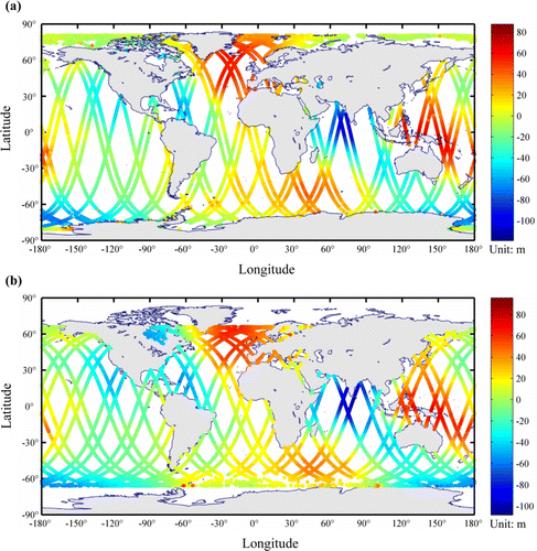
demonstrates the SSH from HY-2 and Jason-2. The SSH inverted from HY-2 agree well with the SSH from Jason-2. In the West Pacific and the North Atlantic, SSH is larger than other ocean areas, while in the Indian Ocean, the SSH is smaller.
Figure 1. Comparison of the sea surface height from the HY-2 and Jason-2 altimeters. (a) HY-2 altimeter SSH; (b) Jason-2 altimeter SSH.
3.1.2. Significant wave height
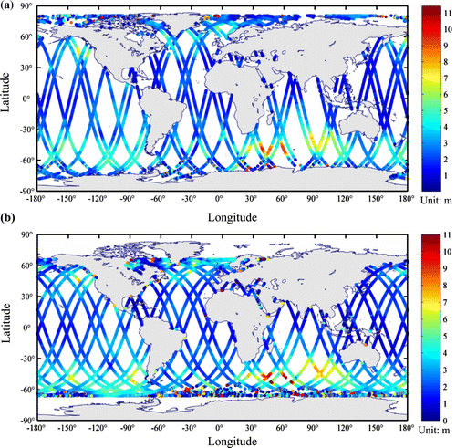
gives a comparison of the SWH from HY-2 and that from Jason-2 satellite radar altimeters. Obviously, in the Southern Ocean, the SWH is higher than other ocean areas, especially the Westerlies. This characteristic is consistent between HY-2 and Jason-2.
Figure 2. Comparison of the SWH from HY-2 and Jason-2 altimeters. (a) HY-2 altimeter SWH; (b) Jason-2 altimeter SWH.
3.1.3. WS
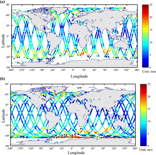
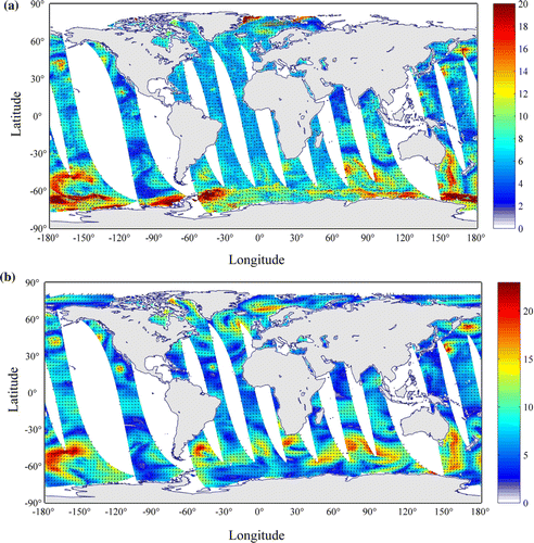
gives a comparison of the WS from HY-2 and Jason-2 satellite radar altimeters. The results show that the HY-2 WS agrees very well with the Jason-2 WS. This characteristic is shared by HY-2 and Jason-2, especially in the Westerlies.
Figure 3. Comparison of the WS from HY-2 and Jason-2 altimeters. (a) HY-2 altimeter WS; (b) Jason-2 altimeter WS.
3.2. Results of the HY-2 scatterometer
The last orbit transformation was finished on 28 September 2011. Since then, the HY-2 scatterometer has collected quality backscatter measurements from the ocean and land surfaces for about one month. Here, we give some preliminary results derived from these data.
3.2.1. The stability analysis of σ0
Rain forest is usually regarded as one of the most stable targets on the earth's surface. In order to verify the stability of HY-2 scatterometer backscatter measurements, we selected one Amazon rain forest region as the study target. The longitude range of this region is from –66°E to –60°E, while the latitude range is from –8°N to –5.5°N. The temporal coverage of the σ 0 data is three days, from 17 October to 19 October 2011. gives the σ 0 scatter plots of this rain forest region.
Figure 4. (a) σ 0 scatter plot of the inner beam for an ascending pass; (b) σ 0 scatter plot of the inner beam for a descending pass; (c) σ 0 scatter plot of the outer beam for an ascending pass; (d) σ 0 scatter plot of the outer beam for a descending pass.
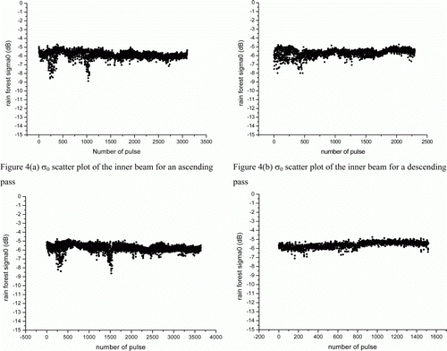
From , it can be seen that the σ 0 measurements in this region fluctuate around a fixed mean value and the variation is very small, which indicates the stability of the instrument. The mean value and the standard deviation of σ 0 measurements for each beam and pass are listed in .
Table 7. Mean value and standard deviation of σ0 for rain forest.
3.2.2. Comparison of the retrieved and NCEP wind field
The comparison between the retrieved wind field and the spatially and temporally matched NCEP wind field can verify the correctness and validity of the scatterometer's σ 0 measurements. (a) and (b) presents the retrieved wind field and the corresponding NCEP wind field for 29 September 2011, respectively. shows that there is high similarity and consistency between these two wind fields as a whole. Especially in the central low area, both wind fields reveal identical cyclone structures with clockwise wind direction.
Figure 5. (a) Wind field retrieved by the HY-2 scatterometer; (b) NCEP wind field.
3.2.3. The capture of a cyclone and front
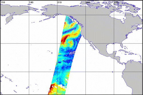
One of the applications of the scatterometer is to exactly capture the diagnostic weather structure, such as cyclones and fronts on the ocean, which are very useful as inputs to enhance the ability of prediction models. gives an example of cyclone and front structure captured by the HY-2 scatterometer. demonstrates that the HY-2 scatterometer is capable of capturing meso-scale weather structures.
Figure 6. Synoptic cyclone and front structure captured by the HY-2 scatterometer.
3.3. Results of the scanning RM
We compared the HY-2 RM data with NCEP re-analysis data. These NCEP FNL (final) operational global analysis data are on 1.0°×1.0° grids produced every six h. These data are from the Global Data Assimilation System (GDAS), which continuously collects observational data from the Global Telecommunications System (GTS) and other data sources for many analyses.
We matched the oceanic geophysical quantity retrieved by the HY-2 RM and NCEP re-analysis data on the global scale from 10 October to 20 October 2011. The time matching scale is 0.5 h and the geographical matching scale is 0.3°. We matched 80,000 points, and calculated the RMS of the two datasets.
Because there has not been much time since the launch of HY-2, and the TBs are not precisely calibrated and the algorithms are not optimized, we believe that the precision of the retrieved oceanic geophysical quantity is fairly satisfactory, and the SSW and WV will be more accurate after the TBs are precisely calibrated in the near future. These results can also prove that the instrument and data processing software work well, as shown in .
Table 8. Comparison of HY-2 RM and NCEP re-analysis products.
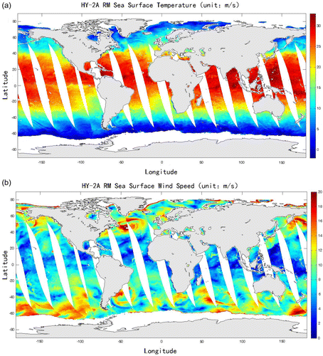
The retrieved oceanic geophysical quantity results of HY-2 RM are shown in .
Figure 7. (a) SST retrieved by the HY-2 RM; (b) wind speed retrieved by the HY-2 RM.
3.4. Results of the HY-2 MOE
3.4.1. GPS MOE accuracy with SLR validation
SLR data used to compare GPS MOE include 11 SLR stations, and the mean accuracy of these SLR data is 2–3 cm. The MOE determined by the GPS tracking system was independently validated by SLR data with one cycle duration. The SLR validation GPS MOE accuracy RMS is about 2.7 cm.
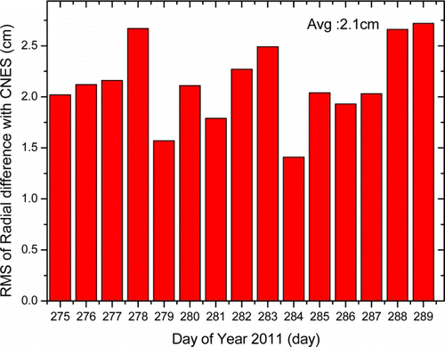
3.4.2. GPS MOE radial difference with CNES
The MOE determined with GPS was compared to that determined by CNES DORIS tracking system with one cycle duration. The RMS of radial difference is illustrated in . We found that the largest RMS of radial difference with CNES'MOE is less than 3 cm and the average of RMS is about 2.1 cm, as shown in .
Figure 8. RMS of radial difference with CNES.
4. Preliminary assessment and conclusion
From the aforementioned preliminary results, it can be concluded that the HY-2 radar altimeter has the ability to measure global SSH, SWH, and WS with high accuracy. A comparison with Jason-2 data shows that the SSH, SWH, and WS results from HY-2 and Jason-2 altimeters are highly consistent. More recently, we have been carrying out CAL/VAL, so it can be expected that more accurate results will be gained after the CAL/VAL program.
From the data analysis results, we can see that the HY-2 scatterometer exhibits high stability in σ 0 measurements and can be used to operationally provide global ocean surface winds for weather prediction models and other uses. However, it must be noted that the absolute calibration of σ 0 has not yet been performed, so better results can be achieved after the in-orbit calibration stage.
The RM can retrieve precise oceanic geophysical parameters and the RM instrument and data processing system work well.
The RMS accuracy of the HY-2 satellite MOE determined by a GPS tracking system with respect to SLR is 2.7 cm, and the RMS of the HY-2 satellite's orbit radial difference compared with CNES is 2.1 cm.
The preliminary results show that the wind vector, SSH, SWH, SST, WS, and MOE are within the designed technical specifications. A further accuracy assessment of HY-2 data will be reported in the future.
Notes on contributors
Xingwei Jiang is a senior scientist at National Satellite Ocean Application Service, SOA. He holds PhD in Ocean University of China. His research interests lie in oceanography, satellite remote sensing and information system.
Mingsen Lin is a senior scientist at National Satellite Ocean Application Service, SOA. He holds PhD in China Academy of Science. His research interests lie in remote sensing of the ocean, computation fluid dynamics.
Jianqiang Liu is a senior scientist at National Satellite Ocean Application Service, SOA. He holds master degree in National Marine Environmental forecasting center, SOA university of China.His research interests lie in remote sensing of the ocean.
Youguang Zhang is a researcher at National Satellite Ocean Application Service, SOA. He holds PhD in Institute of Oceanography, Chinese Academy of Sciences. His research interests lie in remote sensing of the ocean.
Xuetong Xie is a associate researcher at National Satellite Ocean Application Service, SOA. He holds PhD in Peking University. His research interests lie in remote sensing of the ocean.
Hailong Peng is a associate researcher at National Satellite Ocean Application Service, SOA. He holds PhD in Peking University. His research interests lie in remote sensing of the ocean.
Wu Zhou is a research assistant at National Satellite Ocean Application Service, SOA. He holds master degree in National Marine Environmental forecasting center. His research interests lie in remote sensing of the ocean.
Acknowledgements
The project was supported by the National High-Tech Project of China (No. 2008AA09A403) and the Marine Public Welfare Project of China (No. 201105032).
References
- Barrick , D.E. 1972 . Remote sensing of the sea state by radar . Engineering in the Ocean Environment , 9 ( 13 ) : 186 – 192 .
- Barrick , D.E. and Lipa , B.J. 1985 . Analysis and interpretation of altimeter sea echo . Advnces in Geophysics , 27 : 61 – 100 .
- Chi , C.Y. and Li , F.K. 1988 . A comparative study of several wind estimation algorithms for spaceborne scatterometers . IEEE Transactions on Geoscience and Remote Sensing , 26 : 115 – 121 .
- Dunber , R.S. and Hsiao , V.S. , 2001 . Science algorithm specification for SeaWinds on QuikSCAT and SeaWinds on ADEOS-II . California : JPL . Available from: http://podaac.jpl.nasa.gov/quikscat [Accessed October 2003] .
- Freilich , M.H. , 1999 . SeaWinds algorithm theoretical basis document . MD NASA . Available from: http://podaac.jpl.nasa.gov/quikscat/qscat-doc [Accessed May 2003] .
- Moore , R.K. and Williams , C.S. 1957 . Radar terrain return at near-vertical incidence . Proceedings of IRE , 45 ( 2 ) : 228 – 238 .
- Shaffer , S.J. and Dunbar , R.S. 1991 . A median-filter-based ambiguity removal algorithm for NSCAT . IEEE Transactions on Geoscience and Remote Sensing , 29 : 167 – 173 .
- Wentz , F.J. and Gentemann , C. 2000 . Satellite measurements of sea-surface temperature through clouds . Science , 288 : 847 – 850 .
- Witter , D.L. and Chelton , D.B. 1991 . A Geosat altimeter wind speed algorithm and a method for altimeter wind speed algorithm development . Journal of Geo physical Research , 96 : 8853 – 8860 .