Characterization of ASTER GDEM elevation data over vegetated area compared with lidar data

Abstract

Current researches based on areal or spaceborne stereo images with very high resolutions (<1 m) have demonstrated that it is possible to derive vegetation height from stereo images. The second version of the Advanced Spaceborne Thermal Emission and Reflection Radiometer Global Digital Elevation Model (ASTER GDEM) is the state-of-the-art global elevation data-set developed by stereo images. However, the resolution of ASTER stereo images (15 m) is much coarser than areal stereo images, and the ASTER GDEM is compiled products from stereo images acquired over 10 years. The forest disturbances as well as forest growth are inevitable in 10 years time span. In this study, the features of ASTER GDEM over vegetated areas under both flat and mountainous conditions were investigated by comparisons with lidar data. The factors possibly affecting the extraction of vegetation canopy height considered include (1) co-registration of DEMs; (2) spatial resolution of digital elevation models (DEMs); (3) spatial vegetation structure; and (4) terrain slope. The results show that the accurate coregistration between ASTER GDEM and national elevation dataset (NED) is necessary over mountainous areas. The correlation between ASTER GDEM minus NED and vegetation canopy height is improved from 0.328 to 0.43 by degrading resolutions from 1 arc-second to 5 arc-second and further improved to 0.6 if only homogenous vegetated areas were considered.

Keywords:

• vegetation canopy height
• ASTER GDEM
• NED
• photogrammetry
• stereo-mapping

1. Introduction

Digital elevation model (DEM) is essential for the construction of digital earth. Currently, there are two sets of near-global DEM generated from remotely sensed data. One is the elevation data-set produced using the C-band single-pass Interferometry Synthetic Aperture Radar (InSAR) data obtained by the Shuttle Radar Topography Mission (SRTM) (from 56°S to 60°N latitudes). The other is the Global Digital Elevation Model generated by the stereo processing of the Advanced Spaceborne Thermal Emission and Reflection Radiometer Global Digital Elevation Model (ASTER GDEM) covering the earth land surface between 83°N and 83°S latitudes.

Apparently, the 2 sets of DEM are generated by different techniques, i.e. InSAR and photogrammetry, respectively. Vegetation canopy height is a critical parameter in modeling ecosystem processes and carbon cycle (Balzter, Rowland, and Saich 2007; Sexton et al. 2009). It is well known that InSAR is sensitive to the vertical distributions of ground objects. Therefore, there are many researches for the extraction of vegetation height using InSAR data. For example, Hagberg, Ulander, and Askne (1995) found that the penetration depth at C band increased from dense forest to less dense forest when the tree heights were similar. Neeff et al. (2005) used the interferometric height, i.e. the difference of the surface elevations derived from interferometric SAR data at X and P bands to retrieve forest height within a pixel. They found that interferometric height was dependent on the forest succession stage or disturbance history that control vertical and horizontal structures. Balzter, Rowland, and Saich (2007) also presented a method to map vegetation canopy height using dual-wavelength InSAR data at X- and L-band. Kellendorfer et al. (2004) studied the extraction of the forest canopy height from SRTM using the national elevation dataset (NED). Simard et al. (2006) explored the mapping of mangrove forest height in the Everglades National Park using SRTM calibrated by United States Geological Survey (USGS) digital terrain model (DEM) and airborne lidar data. Scientists at the Woods Hole Research Center have produced a high-resolution ‘National Biomass and Carbon Dataset for the year 2000’ (NBCD2000) (Walker et al. 2007), which mainly employed the height of scattering phase center extracted by the difference between SRTM and NED.

Photogrammetry is a traditional technique for the extraction of digital surface model (DSM). The information of vegetation canopy height should be contained in the stereo imagery because it is acquired by optical sensor, which records the signal mainly reflected by top surface of the vegetation canopy. In the past, photogrammetry worked on aerial stereo images and the information of vegetation structure was always suppressed by manual selection of cognominal points under forest in order to get the elevation of ground surface as accurate as possible. Some researchers in the field of surveying and mapping have investigated the extraction of vegetation structure using aerial or spaceborne stereo images. Sheng, Gong, and Biging (2001) successfully reconstructed crown surface of a redwood tree from high-resolution aerial images. Gong et al. (2002) presented a correction method for improvement of the canopy boundary locations in the DSM derived from high-resolution aerial images. Naesset (2002) measured the mean tree height of 73 forest stands in a 1000 ha forest area by automatic stereo processing of aerial images. The mean heights from the stereo imagery underestimated the true heights by 5.42 m. Toutin (2004) reported the results from spaceborne stereo imagery – Ikonos with resolution of 0.8 m. An elevation linear error of 1.5 m was obtained for bare surfaces compared with DEM from Lidar data. St-Onge et al. (2008) created hybrid photo-lidar canopy height models (CHMs) by subtracting the lidar DTM from the aerial photogrammetric DSM. Photo-lidar CHMs were well correlated to their lidar counterparts on a pixel-wise basis but have a lower resolution and accuracy.

These researches demonstrated that photogrammetry (stereo imagery) held great potentials to derive vegetation height. However, most of current researches were conducted on aerial images or spaceborne images with very high resolutions (about 0.5 m). The characteristics of DSMs derived by photogrammetry could be affected by image resolutions because the automatic recognition of cognominal points from stereo images mainly depend on image textures. ASTER has a resolution of 15 m, which is far coarser than aerial images. Therefore, the characteristics of DSM from ASTER data may be different with those from high-resolution image. There are rare researches on the characteristics of DSM from ASTER stereo images over vegetated areas.

The second version of the ASTER GDEM at a spacing of 1 arc-second has been formally released by Japanese Ministry of Economy, Trade and industry (METI) and National Aeronautics and Space Administration (NASA) on 17 October 2011. The first version was produced using almost 1.3 million scenes of ASTER VNIR data acquired from 1999 to 2008. Another 260,000 additional scenes data were used to improve the coverage, and a smaller correlation kernel was used to improve data quality in the second version. The validation report documented that data quality has a great improvement in the second version (Tachikawa et al. 2011). The spatial resolution was improved from about 120 m to about 71–82 m. The number of voids and artifacts were also substantially reduced, and a negative 5 m overall bias was removed. The global altimeter study found that ASTER GDEM was sensitive to tree canopy height. Therefore, the release of ASTER GDEM provides the research community a great opportunity to investigate the feasibility and problems of vegetation canopy height mapping over large areas using ASTER GDEM. More importantly, ASTER GDEM covers larger areas than SRTM, especially for the boreal forest beyond 60°N latitudes.

However, the ASTER GDEM is compiled products from ASTER data acquired over 10 years. The seasonal effects, forest disturbances as well as forest growth are inevitable in 10 years time span. Under this circumstance, this study is mainly to investigate two main problems by comparing ASTER GDEM against lidar data: (1) the possibilities of extracting vegetation canopy height from ASTER GDEM and (2) the method to select effective pixels if not all pixels are useful.

2. Methodology

The extraction of vegetation canopy height from SRTM while taking NED as the elevation of ground surface has been widely investigated and accepted in the United States of America (Simard et al. 2006; Kenyi et al. 2009; Kellndorfer et al. 2010). In this study, NED also serves as the elevation of ground surface. The vegetation canopy height information is investigated in the difference image of ASTER GDEM and NED, i.e. ASTER GDEM minus NED. The analysis requires in situ measurement of vegetation canopy height. Lidar data are the direct measurement of vegetation structures (Lefsky et al. 1999; Sun et al. 2011). Our previous researches were conducted on the first version of ASTER GDEM against the footprint measurement of Geoscience Laser Altimeter System (GLAS) over Chinese Changbai mountainous areas (Ni et al. 2010). The lidar data acquired by the Laser Vegetation Imaging Sensor (LVIS) will provide the measurements of vegetation vertical structures in this study. LVIS developed by NASA Goddard Space Flight Center is an airborne full waveform medium footprint Lidar system (http://lvis.gsfc.nasa.gov/index.html). It has been demonstrated that LVIS provides highly accurate measurements of the forest vertical structure (Blair, Rabine, and Hofton 1999).

As pointed out in the validation report, the horizontal displacement of ASTER GDEM has been improved from 0.95 pixels in the first version to 0.23 pixels in current version. Van Niel et al. (2008) found that the co-registration accuracy should be higher than 0.1 pixels when the difference value between two DEMs was used in the extraction of geophysical parameters. A method for the co-registration of two DEMs has been proposed and validated in our previous researches (Ni et al. 2014). The method will be employed for the co-registration between ASTER GDEM and NED. The co-registration of two DEMs are modeled by a quadratic polynomial, which can consider the transformation caused by horizontal translation, rotation, skew, and scales. Two simulated images will be generated based on the local incidence angle calculated from the two DEMs. The transformation parameters can be calculated based on the control points selected from the simulated images. ASTER GDEM will be resampled to NED using the transformation parameters.

Kellndorfer et al. (2004) found that sample averaging was a critical prerequisite (they recommend around 20 pixels) in the extraction of forest canopy height from SRTM-NED. To examine the effect of resolution on the estimation of forest canopy height, the ASTER GDEM minus NED data were aggregated from 1 arc-second to 5 arc-second at a step of 1 arc-second by averaging.

The results of photogrammetry are determined by the cognominal points recognized from the stereo images. The recognition of cognominal point could be affected by vegetation structures and observation geometry. For homogenous and dense forest, the common points should come from the forest canopy top because the optical image cannot penetrate the forest canopy. For multilayered or sparse forest, the recognition of cognominal point is easily affected by the observation geometry. Over these heterogeneous or sparse forests the cognominal point may be identified in some pairs of stereo images but not in others acquired under different geometry. ASTER GDEM is compiled based on several stereo image pairs. Therefore, the ASTER GDEM over the homogeneous forest is theoretically more stable than over sparse or multilayered forests. A homogeneous index is proposed here to examine whether this is true. The index could be used to select reliable pixels to minimize the influence of vegetation structure on the estimation of vegetation canopy height from ASTER GDEM minus NED. The standard deviation of ASTER GDEM minus NED within a pixel (for pixel size larger than 1 arc-second) or surrounding a pixel (for pixel size of 1 arc-second) is taken as the homogeneous index of the pixel. For the data at the resolution of 1 arc-second, the homogeneous index of a pixel is the standard deviation of ASTER GDEM minus NED within a given window (e.g. 5*5). For other resolutions, the homogeneous index of a pixel is the standard deviation of ASTER GDEM minus NED of those 1 arc-second sub-pixels included in a pixel. For example, for a 2 arc-second pixel, its homogeneous index is defined by the standard deviation of ASTER GDEM minus NED of the corresponding four pixels of 1 arc-second while that of a 3 arc-second pixel is defined by the standard deviation of ASTER GDEM minus NED of the corresponding nine pixels of 1 arc-second. The thresholds of the homogeneous index used in the study were 1–5 m. Only the pixels with the homogeneous index smaller than the threshold were used in analyses.

Slope is an important factor affecting the estimation accuracy of bio-geophysical parameters from remotely sensed data. After the co-registration of ASTER GDEM and NED, the effects of slope on the correlation between ASTER GDEM minus NED and forest canopy height were investigated. A slope threshold was set in the analysis. The pixels with slopes smaller than or equal to the threshold were used in analyses. The threshold was increased from 5° to 60° with a step of 5°.

In all, the factors considered in this study include (1) co-registration of DEMs; (2) spatial resolution of DEMs; (3) spatial vegetation structure; and (4) terrain slope.

3. Test site and data

3.1. Test site

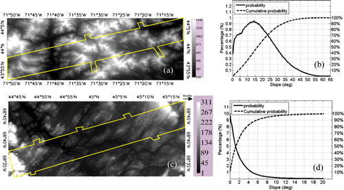
This study is conducted over 2 test sites. One is over mountainous areas (71°40′ W, 44° 0′ N) located between the towns of Warren and Conway in New Hampshire (NH), USA while the other (68°40′ W, 45° 0′ N) is over flat areas between Howland and Bangor in Maine (ME), USA. Figure 1a is the 1 arc-second NED provided by USGS over NH site while Figure 1c is that over ME site. It shows that the elevation ranges from 118 to 1440 m at NH and ranges from 1 to 311 m at ME site. Figure 1b shows the histogram of slopes from Figure 1a. About 30% of the area has slopes smaller than 10°, 60% between 10° and 35°, and 10% higher than 35°. Figure 1d shows the histogram of slopes from Figure 1c. About 90% of the area has slopes smaller than 6°. The polygons on Figure 1a and 1c indicate the area covered by LVIS data.

Figure 1. The terrain conditions of test sites. (a) 1 arc-second national elevation dataset (NED) at New Hampshire site (NH); (b) the probability and cumulative probability frequency (dotted line) of terrain slope at NH; (c) 1 arc-second NED at Maine site (ME); (d) the probability and cumulative probability frequency (dotted line) of terrain slope at ME. The polygons on (a) and (c) indicate the area covered by LVIS data.

The NH site is featured with old-growth northern hardwoods (Lee et al. 2011). The dominant species include beech, yellow birch, sugar maple, and eastern hemlock. In lower elevations, most of the forest is covered by tall canopies where sugar maple/beech/yellow birch dominates the upper canopy layer. At higher elevation before reaching the forest line, spruce, fir, and hemlock are commonly mixed with hardwoods, and can be dominant on cool steep slopes (Filip and Little 1971). Ten percent area is covered by young forest lower than 12 m, 80% is forest between 12 and 32 m, and 10% forest is higher than 32 m. The peak of probability distribution of forest height is around 24 m.

The ME site is currently used for interdisciplinary forest research and experimental forestry practices. The natural stands in this northern hardwood boreal transitional forest consist of hemlock-spruce-fir, aspen-birch, and hemlock-hardwood mixtures. The dominant species include quaking aspen, paper birch, eastern hemlock, red spruce, balsam fir, and red maple (Huang et al. 2013). This site has an American Flux Tower within intermediate aged forest, and the surrounding areas are private land owned by a timber production company with different forest management manipulations such as clear-cut, select-cut, and stripe-cut (Huang et al. 2013). Twenty percent area is covered by young forest lower than 10 m, 70% is intermediate aged forest between 10 and 23 m, and 10% matured forest higher than 23 m. The peak of probability distribution of forest height is around 20 m.

3.2. Data

ASTER GDEM is released in geotiff format with geographic lat/long coordinates and at 1 arc-second (approximately 30 m) grid. The latitude-longitude coordinate of ASTER GDEM is referenced to the World Geodetic System 1984 (WGS 84), and the elevations are computed with respect to the Earth Gravitational Model 1996 (EGM96 geoid) (Slater et al. 2009). The software (GEOTRANS) developed by the National Geospatial-Intelligence Agency can calculate the differences between EGM96 geoid and the ellipsoid surface of Geodetic Reference System 1980 (GRS 80). ASTER GDEM has been transformed to the ellipsoid surface of GRS80 before analysis.

The NED is a seamless elevation dataset for the continental United States provided by USGS from a compilation of various data sources with some dating back as far as 1978 (Gesch et al. 2002; Kenyi et al. 2009). The NED released in geographic coordinates at a resolution of 1 arc-second is selected in this study for the consistent spatial resolution of the different elevation data sets. The horizontal reference of NED DTM is North American Datum 83 (NAD83) while that of vertical is the North American Vertical Datum of 1988 (NAVD 88). The tool GEOID12 developed by National Geodetic Survey (NGS) was used to transform NED data to the ellipsoid surface of GRS80 from NAVD 88. The overall absolute vertical accuracy of the NED expressed as the root mean square error (RMSE) is 2.44 meters estimated with the National Geodetic Survey control points (http://ned.usgs.gov/downloads/documents/NED_Accracy.pdf).

NASA's LVIS is an airborne laser altimeter system designed, developed, and operated by the Laser Remote Sensing Laboratory at Goddard Space Flight Center (http://lvis.gsfc.nasa.gov/index.html). The LVIS data used in this study were acquired on August 2009 with a footprint size of 20 m for both NH and ME sites. LVIS Ground Elevation (lge) data include location (latitude/longitude), ground surface elevation, and the heights of energy quartiles (relative height to ground surface, RH25, RH50, RH75 and RH100) where 25%, 50%, 75%, and 100% of the waveform energy occur. The elevation is referred to the WGS-84 (i.e. GRS80) ellipsoid. The quartile heights are the relatively direct measurement of the vertical profile of canopy components. The RH50 and RH100 of LVIS data for the study area were both rasterized to 1 arc-second ×1 arc-second pixels. The RH50 and RH100 of footprints located within a pixel were averaged respectively to be the value of the pixel. The pixels having no footprints are masked out and not included in the analysis.

The lidar waveform from flat bare ground has only 1 Gaussian peak, which should be located at the ground surface, and the RH50 should theoretically be zero because lidar waveform is symmetric around the ground peak. If vegetation appears within lidar footprint, H50 should be greater than zero due to the more contributions from vegetations above ground surface. In this study, pixels having RH50 greater than 0.5 m (instead of zero) are taken as vegetated areas considering the effects of noise and waveform extension caused by terrain slopes. The comparison will be made between ASTER GDEM minus NED and RH100, which is the measurement of vegetation canopy top height.

4. Results

Figure 2 shows the difference image between ASTER GDEM and NED, and vegetation canopy height map (RH100) from LVIS data. Figure 2a and 2c covers the same area with Figure 1a while Figure 2d and 2e covers the same area with Figure 1c. Figure 2a is the difference between original ASTER GDEM and NED while Figure 2b is that between co-registered ASTER GDEM and NED at NH site. Figure 2c is the RH100 from LVIS. The polygons in Figure 2a and 2b is the area covered by LVIS. Table 1 shows the transformation parameters for the co-registration of ASTER GDEM to NED. Besides other deformation parameters, the displacement between ASTER GDEM and NED at longitude direction is 1.06 pixels while that on latitude direction is 0.162 pixels. The terrain features caused by mis-registration between ASTER GDEM and NED are explicit in Figure 2a. The image of slopes facing to north is white while that on slopes facing to opposite direction is dark. ASTER GDEM is higher on north slopes and lower on south slope than NED because ASTER GDEM shifted to north relative to NED due to mis-registration. Most of these features have been successfully removed after the co-registration of ASTER GDEM and NED. The spatial pattern on Figure 2b within the polygon is similar to Figure 2c. Figure 2d is the difference between original ASTER GDEM and NED at ME site while Figure 2e is corresponding LVIS data. No obvious terrain features as in Figure 2a are observed. The spatial pattern in Figure 2d resembles that in Figure 2e in a certain degree.

Figure 2. The difference images between ASTER GDEM and NED; (a) the difference between original ASTER GDEM and NED (NH site); (b) the difference between registered ASTER GDEM and NED (NH site); (c) RH100 from LVIS data (NH site); (d) the difference between original ASTER GDEM and NED (ME site); (e) RH100 from LVIS data (ME site). The polygons on (a), (b), and (d) are the area covered by LVIS.

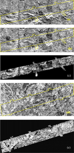
Table 1. The affine parameters for ASTER GDEM relative to NED.

Translation vector (pixel)			Scale vectors			Accuracy (pixel)
Latitude direction	Longitude direction	Skew	Latitude direction	Longitude direction	Rotation (degree)	Latitude direction	Longitude direction
0.162	1.060	−0.00076	0.9975	0.9996	1.57e^−3	0.089	0.094

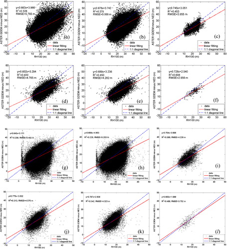
Figure 3 shows the scatter plot of RH100 against the difference between ASTER GDEM and NED after co-registration. The first 2 rows are for NH site while the last 2 rows are for ME site. The first and third rows are the results at the resolution of 1 arc-second while the second and forth rows are the results at the resolution of 5 arc-second. The homogenous index is not applied on the left column. The middle and right columns are the results under the homogenous index of 5 and 1 m, respectively. It is clear that the R² increases while RMSE decreases with the data resolution going coarser. For NH site, the R² improved from 0.328 to 0.430 while RMSE is reduced from 5.76 to 4.76 m when the resolution changed from 1 arc-second to 5 arc-second. The homogenous index performs well in selecting effective pixels. R² increases while RMSE decreases with smaller homogenous index (more homogeneous). As shown in the first row figures in Figure 3, the R² is improved from 0.328 to 0.45 while RMSE is reduced from 5.76 to 3.95 m when a 1 m threshold of homogenous index was used. The results at ME site show the same phenomenon described above.

Figure 3. The effect of resolution and homogenous index on the correlation between ASTER GDEM minus NED and RH100. The first two rows (i.e. a–f) are for NH site while the last two rows (i.e. g–l) are for ME site. For each site the first row is the result of 1 arc-second while the second row is that of 5 arc-second. The homogenous index is not applied on the left column. The homogenous index applied on the middle column is 5 m while that on the left column is 1 m.

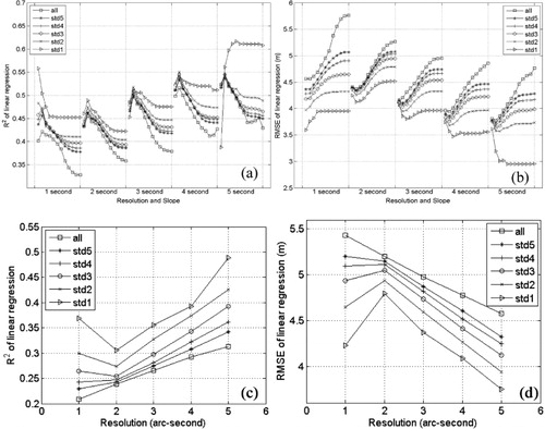
Figure 4 shows the effects of resolution, slope, and vegetation structure on the correlation between ASTER GDEM minus NED and vegetation canopy height. Figure 4a and 4b is the R² and RMSE of linear regression between ASTER GDEM minus NED and RH100 at NH site, respectively. The six lines stand for whether the homogenous index is applied and the value of homogenous index applied. ‘all’ means the homogenous index is not applied. ‘std5’ means the homogenous index applied is equal to 5 m. As described in methodology, the slope threshold under each resolution increases from 5° to 60° with a step of 5°. It can be seen that R² increases gradually from 1 arc-second to 5 arc-second under each requirement of homogenous index while RMSE decreased gradually. The R² goes up and RMSE goes down with the homogenous index becoming stricter under each resolutions. The forest stands located under 10° slopes has the best correlation between ASTER GDEM minus NED and RH100 under nearly all data resolutions and homogenous index but that of std1 under 5 arc-second. The correlation becomes worse after the slopes threshold exceed 10°. Figure 4c and 4d are the R² and RMSE of the linear regression model at ME site. The effects of slope are not explored at ME site due to the narrow dynamic ranges of slopes. The results at ME repeat the same phenomenon exhibited at NH site in terms of resolution and homogenous index. The correlation between ASTER GDEM minus NED and RH100 becomes better as pixel size goes larger or vegetation becomes more homogenous.

Figure 4. The effects of resolution, slope, and vegetation structure on the correlation between ASTER GDEM minus NED and vegetation canopy height. (a) and (b) are R² and RMSE of the linear regression for NH site, respectively; the slope threshold increases from 5° to 60° at a step of 5° (left to right) in each resolution; (c) and (d) are R² and RMSE of the linear regression for ME site, respectively. The std1 to sd5 are for the cases of using 1–5 meters as the threshold of homogeneous index. The ‘all’ means no limit on the homogeneous index.

5. Discussions

It has to be pointed out that the homogeneous index used in the analysis is directly calculated from ASTER GDEM minus NED rather than LVIS data. The limited availability of LVIS data will limit the application of the proposed method if it is calculated from LVIS data although it is more accurate on the description of vegetation homogeneity than ASTER GDEM minus NED. The proposed method provides us a practical way to refine the correlation between ASTER GDEM minus NED and vegetation canopy height.

Figure 4 shows that a case of deviance occurred at 5 arc-second and 1 m homogenous index at flat area (slope < 5°). The R² is low and RMSE is high in this case. That is mainly due to the fact that too few pixels were remained under such coarse resolution and such strict requirements.

Another issue is the uncertainty of the time span between ASTER stereo images used to produce ASTER GDEM over the test area. Forest disturbance or growth may happen if the time span is too long. If the time span is known over the test area, the overall accuracy may be improved by excluding the disturbed pixels or by considering the uncertainty caused by forest growth. The time span information generally cannot affect the analysis on resolution, slope, and DEMs co-registration in this study. It may have some influences in the effect of forest homogeneity but the influences should be positive because the consideration of forest disturbance can help us to exclude false homogenous forest pixels.

The results of co-registration between NED and ASTER GDEM show an obvious displacement between them at NH site. Co-registration of DEMs is a very important prerequisite of DEM validation and the application of the difference between 2 or more DEMs especially over mountainous areas. The value of transformation parameters given in Table 1 may give us an impression that the horizontal translation is dominant and others can be neglected because they are far smaller than the translation vector. In fact, this is not the case. The effect of skew, scale, and rotation is proportionate to the image size. For example, ASTER GDEM and NED are co-registered under 1 arc-second resolution in this study. The image size is 2414 samples by 864 lines at NH site. The displacement on image edge caused by scaling factor at latitude direction is about 1.079 (864/2*[1–0.9975]) pixels. Therefore, the translation vector alone cannot fully model the deformation of 2 DEMs.

The influences of 4 factors on the correlation between ASTER GDEM minus NED and vegetation canopy height were investigated in this study. DEMs coregistration is undoubtedly a necessary step over mountainous area. Figure 3a shows that the sensitivity of ASTER GDEM minus NED to vegetation canopy height definitely exist although the R² is only 0.328 while RMSE is only 5.765 m. Figure 4 shows the separate or comprehensive effects of slope, resolution, and vegetation structure on the refinement of ASTER GDEM minus NED pixels. It guides users to select effective pixels or determine the proper resolutions according to the requirement of their specific applications. The pixels on flat area have higher accuracy; the pixels of more homogenous forest give more reliable correlations; the bigger mapping unit (resolution) gives more stable results. Although the refinement of ASTER GDEM minus NED excludes the mapping of vegetation canopy height over large areas at high resolution (1 arc-second), the pixels (areas) identified by the criteria (slope, homogeneity, resolution) described in this study can be used as sampling areas for cross validation of vegetation canopy height products from other data sources.

6. Conclusion

The feasibility and critical factors in the mapping or estimation of vegetation canopy height using ASTER GDEM and NED are investigated. The co-registration of DEMs is proven to be the foundation of the application of ASTER GDEM over mountainous areas. The results showed that it was possible to map vegetation canopy height at 1 arc-second for those applications whose accuracy requirement was not very high. Resolution was an important factor for determining the mapping accuracy of vegetation canopy height. Users could select the proper product resolution according to their specific application. Terrain slope also had obvious impact on the mapping accuracy of vegetation canopy height. The pixels on flat area had higher accuracy. But it was not a destructive factor. The mapping of forest canopy height was still feasible even if the effect of slope was not considered. A homogenous index derived from ASTER GDEM minus NED was proposed to describe the homogeneity of vegetation structures. The results demonstrate that it could help to refine effective pixels in the estimation of vegetation canopy height. In all, it was feasible to map forest canopy height using ASTER GDEM with the help of NED. Additional requirements on 3 factors (resolution, slope, and homogenous index) could help to improve the mapping or estimation accuracy of forest canopy height using ASTER GDEM. The uncertainty caused by the long time span of ASTER data is one main limitation in the application of ASTER GDEM for the extraction of vegetation canopy heights. The issue will be fully investigated in future by use of the ASTER stereo images over long time span over various forested areas.

Acknowledgements

This work was partially supported by the National Basic Research Program of China (Grant no.2013CB733404), the National Natural Science Foundation of China (Grant nos. 41001208 and 91125003), support for the study was also provided by the NASA Terrestrial Ecology Program (NNX09AG66G). The LVIS data sets were provided by the Laser Vegetation and Ice Sensor (LVIS) team in the Laser Remote Sensing Laboratory at NASA Goddard Space Flight Center with support from the University of Maryland, College Park. The authors thank each of the foregoing. Special thanks to the ASTER GDEM team and USGS for the open data access.

References

- Balzter, H., C. S. Rowland, and P. Saich. 2007. “Forest Canopy Height and Carbon Estimation at Monks Wood National Nature Reserve, UK, Using Dual-wavelength SAR Interferometry.” Remote Sensing of Environment 108 (3): 224–239. doi:10.1016/j.rse.2006.11.014.
- Blair, J. B., D. L. Rabine, and M. A. Hofton. 1999. “The Laser Vegetation Imaging Sensor (LVIS): A Medium-altitude, Digitations-only, Airborne Laser Altimeter for Mapping Vegetation and Topography.” ISPRS Journal of Photogrammetry and Remote Sensing 54: 115–122. doi:10.1016/S0924-2716(99)00002-7.
- Filip, S. M., and E. L. Little. 1971. Trees and Shrubs of the Bartlett Experimental Forest. Carroll County, New Hampshire: Northeastern Forest Experiment Station, Forest Service, US Department of Agriculture.
- Gesch, D., M. Oimoen, S. Greenlee, C. Nelson, M. Steuck, and D. Tyler. 2002. “The National Elevation Dataset.” Photogrammetric Engineering and Remote Sensing 68 (1): 5–11.
- Gong, P., X. L. Mei, G. S. Biging, and Z. X. Zhang. 2002. “Improvement of an Oak Canopy Model Extracted from Digital Photogrammetry.” Photogrammetric Engineering and Remote Sensing 68 (9): 919–924.
- Hagberg, J. O., L. M. H. Ulander, and J. Askne. 1995. “Repeat-pass SAR Interferometry Over Forested Terrain.” IEEE Transactions on Geoscience and Remote Sensing 33 (2): 331–340. doi:10.1109/36.377933.
- Huang, W. L., G. Q. Sun, R. Dubayah, B. Cook, P. Montesano, W. J. Ni, and Z. Y. Zhang. 2013. “Mapping Biomass Change after Forest Disturbance: Applying LiDAR Footprint-derived Models at Key Map Scales.” Remote Sensing of Environment 134: 319–332. doi:10.1016/j.rse.2013.03.017.
- Kellndorfer, J., W. S. Walker, L. Pierce, C. Dobson, J. A. Fites, C. Hunsaker, J. Vona, and M. Clutter. 2004. “Vegetation Height Estimation from Shuttle Radar Topography Mission and National Elevation Datasets.” Remote Sensing of Environment 93 (3): 339–358. doi:10.1016/j.rse.2004.07.017.
- Kellndorfer, J. M., W. S. Walker, E. LaPoint, K. Kirsch, J. Bishop, and G. Fiske. 2010. “Statistical Fusion of Lidar, InSAR, and Optical Remote Sensing Data for Forest Stand Height Characterization: A Regional-scale Method Based on LVIS, SRTM, Landsat ETM Plus, and Ancillary Data Sets.” Journal of Geophysical Research-Biogeosciences 115: G00E08, 01–10. doi:10.1029/2009JG000997.
- Kenyi, L., R. Dubayah, M. Hofton and M. Schardt. 2009. “Comparative Analysis of SRTM-NED Vegetation Canopy Height to LIDAR-derived Vegetation Canopy Metrics.” International Journal of Remote Sensing 30(11): 2797–2811. doi:10.1080/01431160802555853.
- Lee, S., W. Ni-Meister, W. Z. Yang, and Q. Chen. 2011. “Physically Based Vertical Vegetation Structure Retrieval from ICESat Data: Validation Using LVIS in White Mountain National Forest, New Hampshire, USA.” Remote Sensing of Environment 115(11): 2776–2785. doi:10.1016/j.rse.2010.08.026.
- Lefsky, M. A., W. B. Cohen, S. A. Acker, G. G. Parker, T. A. Spies, and D. Harding. 1999. “Lidar Remote Sensing of the Canopy Structure and Biophysical Properties of Douglas-Fir Western Hemlock Forests.” Remote Sensing of Environment 70 (3): 339–361. doi:10.1016/S0034-4257(99)00052-8.
- Naesset, E. 2002. “Determination of Mean Tree Height of Forest Stands by Digital Photogrammetry.” Scandinavian Journal of Forest Research 17 (5): 446–459. doi:10.1080/028275802320435469.
- Neeff, T., L. V. Dutra, J. R. dos Santos, C. D. Freitas, and L. S. Araujo. 2005. “Tropical Forest Measurement by Interferometric Height Modeling and P-band Radar Backscatter.” Forest Science 51 (6): 585–594.
- Ni, W., Z. Guo, G. Sun and H. Chi. 2010. Investigation of Forest Height Retrieval Using SRTM-DEM and ASTER-GDEM. IEEE International Geoscience and Remote Sensing Symposium, Honolulu, USA, 2111–2114.
- Ni, W., G. Sun, Z. Zhang, Z. Guo and Y. He. 2014. “Co-registration of Two DEMs: Impacts on Forest Height Estimation from SRTM and NED at Mountainous Areas.” IEEE Geoscience and Remote Sensing Letters 11 (1): 273–277. doi:10.1109/LGRS.2013.2255580
- Sexton, J. O., T. Bax, P. Siqueira, J. J. Swenson, and S. Hensley. 2009. “A Comparison of Lidar, Radar, and Field Measurements of Canopy Height in Pine and Hardwood Forests of Southeastern North America.” Forest Ecology and Management 257 (3): 1136–1147. doi:10.1016/j.foreco.2008.11.022.
- Sheng, Y. W., P. Gong, and G. S. Biging. 2001. “Model-based Conifer-crown Surface Reconstruction from High-resolution Aerial Images.” Photogrammetric Engineering and Remote Sensing 67 (8): 957–965.
- Simard, M., K. Q. Zhang, V. H. Rivera-Monroy, M. S. Ross, P. L. Ruiz, E. Castaneda-Moya, R. R. Twilley, and E. Rodriguez. 2006. “Mapping Height and Biomass of Mangrove Forests in Everglades National Park with SRTM Elevation Data.” Photogrammetric Engineering and Remote Sensing 72 (3): 299–311.
- Slater, J. A., B. Heady, G. Kroenung, W. Curtis, J. Haase, D. Hoegemann, C. Shockley, and K. Tracy. 2009. Evaluation of the New ASTER Global Digital Elevation Model. Reston, VA: National Geospatial-Intelligence Agency.
- St-Onge, B., C. Vega, R. A. Fournier, and Y. Hu. 2008. “Mapping Canopy Height Using a Combination of Digital Stereo-photogrammetry and Lidar.” International Journal of Remote Sensing 29 (11): 3343–3364. doi:10.1080/01431160701469040.
- Sun, G., K. J. Ranson, Z. Guo, Z. Zhang, P. Montesano, and D. Kimes. 2011. “Forest Biomass Mapping from Lidar and Radar Synergies.” Remote Sensing of Environment 115 (11): 2906–2916. doi:10.1016/j.rse.2011.03.021.
- Tachikawa, T., M. Kaku, A. Iwasaki, D. Gesch, M. O. Z. Zhang, J. D. T. Krieger, B. Curtis, et al. 2011. ASTER Global Digital Elevation Model Version 2 – Summary of Validation Results. Tokyo: the Joint Japan-US ASTER Science Team.
- Toutin, T. 2004. “DTM Generation from IKONOS In-track Stereo Images Using a 3D Physical Model.” Photogrammetric Engineering and Remote Sensing 70 (6): 695–702.
- Van Niel, T. G., T. R. McVicar, L. T. Li, J. C. Gallant, and Q. K. Yang. 2008. “The Impact of Misregistration on SRTM and DEM Image Differences.” Remote Sensing of Environment 112 (5): 2430–2442. doi:10.1016/j.rse.2007.11.003.
- Walker, W. S., J. M. Kellndorfer, E. LaPoint, M. Hoppus and J. Westfall. 2007. “An Empirical InSAR-optical Fusion Approach to Mapping Vegetation Canopy Height.” Remote Sensing of Environment 109 (4): 482–499. doi:10.1016/j.rse.2007.02.001.