Application of geovisual analytics to modelling the movements of ruminants in the rural landscape using satellite tracking data

Abstract

Geovisual analytics provides a framework for the development of decision support tools for landscape design, analysis and optimisation. An important application is modelling the spatial-temporal movements of ruminants and their grazing behaviour using global positioning system (GPS) collar units. This study describes the mapping and analysis of spatial distributions of animal waste products (which correlate with farm nitrogen [N] emissions) and also determination of animal feeding preferences (which correlate with animal welfare and production). Segmentation of local regions of animal N emissions provides support in meeting targets for local and international N leaching and greenhouse gas emissions. An agent-based model was used for pre-screening in order to gain insights into the clustering behaviour of sheep during feeding activities. Subsequent spatial analysis demonstrated that livestock excreta are not always randomly located, but concentrated around highly localised animal gathering points, separated by the nature of the excretion. In a separate study, the statistical significance of feeding choices was determined by testing a null hypothesis on animal boundary transitions between adjacent pastures using the binomial approximation. The analysis also included compensation for the precision of the GPS sensor, which produced a fuzzy decision boundary.

Keywords:

• agent-based modelling
• geovisual analytics
• nitrogen emissions
• feeding preferences
• ruminants
• satellite tracking

1. Introduction

1.1. Aims of study

A geovisual analytics framework is described for use as a decision support aid for analysis of spatio-temporal movements of ruminants over a rural landscape. The framework includes initial pre-screening and visualisation, using an agent-based approach, followed by numerical and statistical analysis to support inferences from the data. More specifically, application to mapping and analysis of spatial distributions of ruminant waste products is described, as this provides inputs for estimates of biomass data required in models of nitrogen (N) emissions. A methodology is described for the determination of the feeding preferences of ruminants under conditions of spatial uncertainty in satellite tracking data.

Tracking and analysis of the movements of grazing animals in paddocks provides inputs for improving landscape design, and farming practices, with possible economic impacts (product quality, stock numbers and profit), environmental impacts (soil quality and management of N emissions) and animal welfare (including food supply, health and longevity). The need for geovisual analytics is based on the large amounts of multi-dimensional data in space and time, which suggests the need for appropriate visualisation at the human–computer interface together with spatial-statistical analysis.

1.2. Background

Tracking and analysing the movement of animals in their ambient environment provides information for improved landscape design and farming practices. Studies have shown that the behaviour of ruminants grazing on different parts of large paddocks can be affected by various factors, such as aspect, elevation, time of day, pasture mass and quality variation, shade, shelter, watering and supplementary feeding sites (Mayer et al. 1999; Silanikove 2000; Betteridge et al. 2010). In particular, correlation of animal movements with feeding preferences offers the prospect of pasture selection with the aim of production optimisation by nutritional selection. For example, dietary preferences and certain pastures can result in an over-active thyroid gland leading to higher body temperature and sensitivity to heat stress (Silanikove 2000). There is therefore a case for tracking and analysing the behaviour of grazing animals and their interactions with the local environment in order to identify opportunities to improve conditions through redesign of the paddock.

Waste products from grazing ruminants, whilst adding to greenhouse gas (GHG) emissions, can lead to critical source areas (CSAs) that emit a disproportionate amount of N to the environment, especially as leached N can contaminate groundwater (Betteridge et al. 2010; Betteridge 2010). Preferential grazing on different parts of large paddocks can be affected by various factors, such as type of pasture and the time of year. The type of knowledge sought by the analyst could include the pattern of tracks produced by the grazing animals, their flocking sites and frequent locations, especially in times of environmental stress. Gathering sites, in particular, may reveal localised areas of excretion events leading to N leaching and nitrous oxide emissions under certain conditions (e.g. compacted and wet soil).

In the case of gathering areas for excretion, there is a distinction between urination sites and defecation sites (Betteridge et al. 2010). By knowing their relative areas and locations, the estimated mass of excreta can be used to support computer models for the prediction of CSAs and, therefore, N emissions. This would contribute to a mitigation strategy related to N emissions arising from grazing livestock, especially if mitigations are targeted at CSAs (Betteridge et al. 2011). The N losses are mainly in the form of gaseous losses to the atmosphere and leaching into the groundwater (Betteridge et al. 2010). Farmers require information on N losses in order to reduce emissions to meet local and international N leaching and GHG target levels.

Mapping and analysis of animal movement patterns, in response to environmental conditions, provides information for landscape design and optimisation, and could be used to identify feeding preferences. Tracking sheep movements and gathering points provides quantitative information that may be useful to guide the process of paddock design. Optimisation of landscape design in rural production in general may require cost–benefit analysis as well as a comprehensive model for the performance index (Benke and Benke 2013). Examples of factors in landscape design include the following:

• trees location for protection from wind and solar radiation

• hedgerow orientation for wind protection in winter

• area of shade-cloth, orientation and location

• water sources available and location

There are also geometrical design variables to consider, such as paddock slope, perimeter and shape. All these factors may affect farm economics assessment, as they form part of the cost-base. These factors may also influence the location of gathering sites and feeding preferences of grazing animals and therefore contribute to animal welfare, as well as production.

2. Animal tracking and modelling

The combination of an orthogonal temporal axis with two spatial dimensions, together with a global positioning system (GPS), or other tracking technologies, such as video, or a wireless local area network, provides potentially very effective tools for analysis of 3D movement patterns. Digital image processing can reveal bottlenecks and frequently used corridors, which reveal indications of flock behaviour or random grazing (Djordjevic et al. 2008). Monitoring by GPS may show evidence of flocking size, meeting places or periodic patterns and frequented locations (Kreveld, Speckmann, and Gudmundsson 2007; Djordjevic et al. 2008; Gudmundsson, Laube, and Wolle 2008). Evidence of emergent patterns in space and time can be elicited using agent-based models (ABMs), especially if applied to animal models of behaviour (Laube and Dennis 2006; Andersson et al. 2008; Benke et al. 2012).

The use of geovisual analytics enhances the visual perception of meaningful spatial patterns, such as textures, trends or clustering or uncertainty in spatial data that may be less apparent in large numerical arrays and databases (Brown et al. 2005; Benke and Pelizaro 2010; Benke, Pettit, and Lowell 2011). Geovisual analytics may also combine software tools with dynamic methods for analytical reasoning about geographical data, providing tools for inferences from multimodal information sources.

Spatial data mining is aimed at finding patterns in landscapes and geography over space and time using spatial viewers, such as Google Earth. The huge increase in geographically referenced data requires a blend of information technology, digital mapping and remote sensing. A feature of data mining is the automatic search for hidden patterns in large multi-dimensional databases. A variety of data mining techniques can be used in combination with the spatial data to quantify processed information (Kantardzie 2003; Mucherino, Papajoirgji, and Pardalos 2009). This combination of advanced graphics and statistics may include cluster analysis, time-series analysis and digital image processing (including thresholding, segmentation and classification).

In the case of grazing animals, the type of knowledge sought by the analyst could include flocking sites and frequent locations, indicating feeding preferences. Modelling the determinants of sheep behaviour can use data acquired from spatial data layers (e.g. land use, soil, slope, aspect) and observation and monitoring of sheep attributes (breed, weight, age, sex). Data mining techniques are useful for detection of trends, clusters and behavioural patterns in animal interactions and movements across a paddock.

3. Methods

3.1. ABM

An ABM can be used to identify clusters of sheep locations in a preliminary screening of the data on animal movements. It may also be used for studying the effect on cluster location due to changes in system parameters and data. In recent years, agent-based simulation and landscape optimisation have been described as possible tools for analysing changes in space and time due to the complex interaction of ruminants and pastures in an uncertain environment (see recent reviews by Tang and Bennett 2010; Sposito et al. 2010). Multi-agent simulation, using an ABM, involves a combination of factors within a defined framework and consists of the following elements

• autonomous agents

• decision-making rules

• an interaction framework

• data from the surrounding environment

as described schematically in Figure 1 (see also Brown et al. 2005; Mucherino, Papajoirgji, and Pardalos 2009; Tang and Bennett 2010; Benke et al. 2012). An ABM of sheep behaviour can be calibrated using visual analytic techniques in order to predict behaviour under different conditions, for example, varying sheep population density and variations in paddock size and shape.

Figure 1. Schematic diagram of a global modelling framework incorporating an ABM for simulating space-time behaviour of ruminants (see Benke et al. 2012).

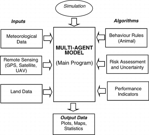
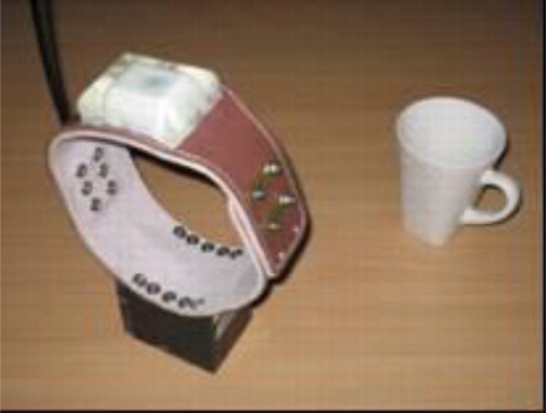
ABMs of sheep can also be combined with simulation techniques for the purpose of predictive modelling (Mucherino, Papajoirgji, and Pardalos 2009). The GPS coordinates can be correlated with environmental data, such as temperature, humidity, solar radiation, wind, mortality, reproduction rates, locations for feeding, drinking and excretion and landscape features. An example of a GPS unit designed for use with sheep is shown in Figure 2. The data-set is stored as a relational database and processed using visual analytics and data mining. Spatial movement is often represented by simple rules based on geometry and Newtonian kinematics. In the context of the current paper, the ABM is used for basic screening of animal movements to identify possible clusters of sheep locations. Further analysis is then carried out using numerical and statistical approaches.

Figure 2. Example of a GPS collar receiver for tracking animal movements (AgTrax II unit from Alana Ecology). Unit consists of antenna and moulding with radio modem, flash memory for up to 65,000 locations and embedded battery pack.

3.2. Clustering, feature extraction and segmentation

The distance between clusters can be determined numerically as the difference between centroids. Visualisation and identification of clusters is possible by thresholding applied to the z-axis for feature extraction and area segmentation. A feasible linear movement in a sub-trajectory may be represented by a change in the so-called four-vector representing to its spatial-temporal location. Total distance travelled is the sum of the sub-trajectory displacements. The total path length, d_t, or trajectory, for an animal is the sum of all the sub-trajectory displacements. This information can be used to provide kinematic data, such as speed and geographic locations, at various times for each animal, while constrained within its spatio-temporal footprint. The approach may be repeated using averages to model the entire flock – allowing monitoring of group behaviour.

(1)

The hypothetical centre-of-mass, C, along a set of points in a one-dimensional sub-trajectory is given by:

(2)

where m_i represents the mass of sheep locations, x_i is the linear coordinate and represents the set of real numbers. When the points are spread out over a plane, the centre-of-mass position as a function of time, t, is described by the vector, r,

(3)

If mass values are equally weighted, that is, m_i = 1 (for i = 1, …, n), the position is referred to as the centroid of the set of coordinates (Johnson 2007). The centre-of-mass and computed areas of excretion sites can be useful for providing frequent-location data for ruminants and also inputs for models estimating animal N emissions.

The centre-of-mass of disparate clusters, together with their areas and shapes, provides information for comparison of homogeneous regions of special interest in 2-D data-sets and digital imagery. Extraction of this information is possible by the operation of thresholding (Singh 1989). For example, in the case of a data array, or image, I(x,y), a threshold, T, can be selected to produce a binary output image with the required information extraction by the following conditional test

(4)

where a and b are both user assigned values, as appropriate,

(5)

(6)

and often take the values [1, 0] respectively in order to form a binary bit image. In digital image processing, the thresholding operation is an example of feature extraction and reveals the area of the object of interest, its shape (contour) and also relative intensity (magnitude information). This operation can be used to partition the image into separate homogenous regions in a process known as segmentation.

3.3. Discrete statistical analysis

Discrete statistical analysis can be used to ascertain the statistical confidence in the computed difference between cluster locations or between animal gathering sites. Consider the case of comparing the mean or centre-of-mass of positions recorded for animals located in two juxtaposed pastures using time-based monitoring by GPS. The null hypothesis, H₀, is that there is no statistically significant difference between the means of the location data in the adjoining paddocks (there is no boundary between the pasture types). One therefore wishes to test this against the alternative hypothesis, that is,

(7)

With the null hypothesis, the statistical difference between the means from the samples, given the sample associated variances, is as follows (e.g. Freund 1998):

(8)

The ratio has increasing statistical significance with increasing z value. For example, the critical value for a particular sample size may be z_crit = 1.645 for a level of significance (los) of α = 0.10. If , the difference in mean values is significant for the specified los and degrees of freedom.

Consider now the case where one deals with proportions rather than mean values. Employing the binomial random variable, X, allows one to use the statistic for the binomial distribution. Once again the null hypothesis is stated, for the proportion of ruminants in a specified paddock,

(9)

For large n, and assuming a normal approximation to the binomial distribution, the decision criterion for preference, p, for a paddock may be assessed by the z-statistic for sample size n (Freund 1998):

(10)

In the current situation, using proportions as a population statistic has advantages, as it allows for total counts in each partition or paddock as the primary metric, without recourse to differences between means, which requires computations of means and variances, as well as total counts. Although clustering and the difference between means is useful in the case of localised distributions of excreta in the landscape (for subsequent estimation of N emissions), it is not required in the case of feeding preference estimation, where estimation of the proportion in a defined paddock area is sufficient. It is also likely that reproducibility and stability in the statistical metric are less of an issue using data on proportions.

4. Experimental results

4.1. ABM

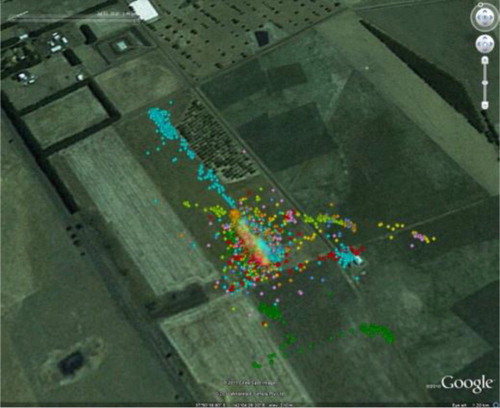
Sheep movements in a paddock at Hamilton, Victoria, are depicted in Figure 3, where seven sheep were tracked in 7 sec time steps using AgTrax II GPS units from the Alana Technology Company with a view to discovering feeding preferences between ryegrass and plantain pastures. The GPS data plus Google Earth imagery in Figure 3 reveals that different sheep are subject to different behaviour patterns, with respect to animal movements, including both solitary exploration and local clustering. Figure 4 is a screenshot of a prototype ABM (Benke et al. 2012), developed using the open source NetLogo software (Wilensky 1999) together with data derived from the DPI farm at Hamilton.

Figure 3. Examples of logged sheep locations over time in a paddock using GPS collars, where each colour tags a specific animal at multiple locations.

Figure 4. Preferred feeding sites for sheep showing clustering from a prototype ABM using NetLogo software (red indicates high density).

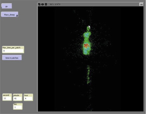
The image depicted in Figure 4 shows cumulative time spent at particular locations. Data were extracted from GPS outputs for sheep over a period of approximately 24 hours at a 7 sec time interval. Green represents at least 1 time step, cyan more than 10 time steps, yellow more than 50 and red more than 100 time steps (red therefore shows preferred feeding areas). This output can therefore be used to identify areas of sheep clusters that could be interpreted as preferred locations. The information processing approach characterising this cluster analysis has one shortcoming in that it still requires formal discrete statistical analysis to provide an indication of confidence or statistical significance.

4.2. Nitrogen emissions

Using data from southern Hawkes Bay, New Zealand, an isometric plot is depicted in Figure 5 showing urination and defecation events, normalised by time, for monitored cows in a paddock in steep hill country (experimental details are described by Betteridge et al. 2010; Betteridge 2010). A sampling grid for the 0.5 ha paddock was used based on GPS data for urine sensor output and defecation data. The data-set was acquired by post-grazing mapping of faeces by GPS of 15 cows grazing the paddock over three days (each cell contains normalised data for time duration, representing cumulative time spent in each grid). Bright orange areas represent urination ‘hotspots’. The contour shape at the base plane represents the perimeter of the paddock boundary fence. The twin peaks represent gathering sites for cows (narrow peak for urination and broad peak for defecation).

Figure 5. Time duration data represented as an isometric projection showing gathering sites for cows.

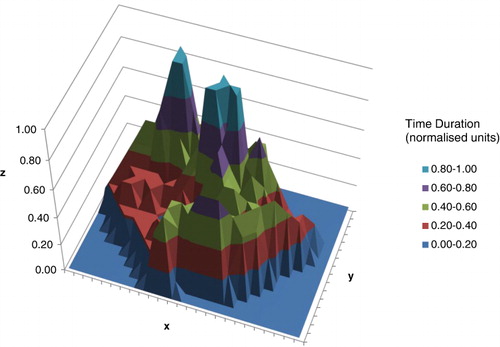
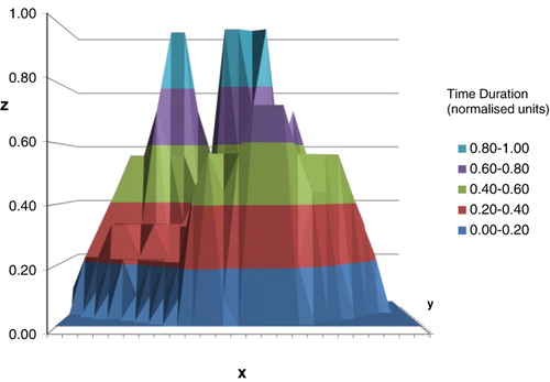
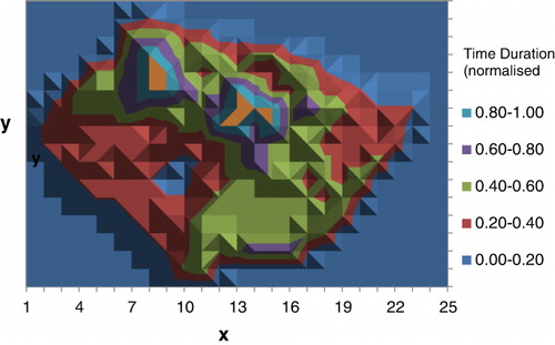
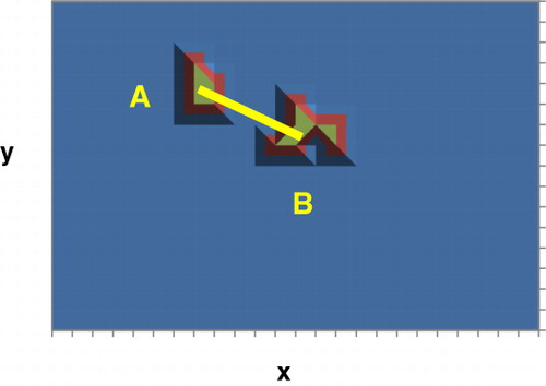
Figure 6 shows the side elevation of the urine and faeces peaks depicted in Figure 5, revealing the degree of peak separation – with the plateau at the base (in blue) providing an indication of relative areas. The rectangular base represents the fenced boundary of the paddock and about 30% of this area contains the excretion patches within the grid cells (thresholding at T = 0.50, or peak full-width at half-maximum, provides two distinct areas for comparative analysis). The area enclosed by the base-line contour represents nearly 50% of the rectangular grid. The patch for defecation was at least 15% larger in area than that used for urination. The side elevation plot demonstrates the power of visual analytics – as trends and clusters not apparent in the original numerical data array can be more easily detected. In Figure 7, the flat plane representation highlights the actual contour of the area used for excretion in a manner suitable for computation. As shown in Figure 8, feature extraction by thresholding was carried out at a level of T = 0.80, revealing more clearly the segmented areas of the peaks and the distance between centroids. In Figure 8, the transect represented by the diagonal line shows the difference between the estimated locations of the centre-of-mass positions for each gathering area, A and B (urine and faeces, respectively), following the operation of thresholding.

Figure 6. Side elevation of twin peaks showing degree of separation of two excretion sites and peak nitrogen emissions. Estimation of peak full-width at half-maximum for each of the peaks provides two distinct areas for comparative analysis.

Figure 7. Flat plane representation of sampled data in the form of a contour plot of normalised time duration for the gathering sites of cows. Bright orange areas represent gathering points for urination.

Figure 8. Clusters from the previous figure have been thresholded (T = 0.80) to separate the peaks from the background. The transect (yellow line) shows the distance between the centre-of-mass positions for areas A and B.

The processed information shows that, in this hill country environment, the locations of natural bodily functions were not randomly distributed, but subject to highly localised gathering points, with different sized areas involved. The areas involved provide inputs for a model-based approach to estimating spatial variation of N emissions due to urination. One application of this work is the estimation of total N load versus dry matter yield, a metric that enables optimum allocation of fertiliser (Betteridge et al. 2010). This recycling of organically sourced fertiliser is a benefit to the farmer as it lowers the cost of commercial fertiliser required for pasture growth.

4.3. Sheep-feeding preferences

4.3.1. Coordinate translations

Spatial analysis and numerical computations may be simplified if certain geometrical transformations are applied to the field data, such as aligning the paddock reference frame to the global reference frame. Rotation and translation of the coordinate system often provides benefit with respect to numerical analysis, for example, converting the reference frame of analysis from 2-D to multiple 1-D views and producing n samples of x-axis data-sets. If p(x,y) is a point in the old reference frame, then transformation of the coordinate into the new reference frame, p'(x',y'), involves a linear translation to a new point, (x₀,y₀), and a clockwise rotation, α, and is given by:

(11)

(12)

where both translation and rotation are canonical transformations (Thomas and Finney 1998). If x₀ = 0 and y₀ = 0, the transformation is a rotation only and simplifies to

(13)

(14)

This approach rotates the paddock image so that the boundaries are parallel with the global coordinate axes, that is, analysis can be simplified by considering the 1-D case only but with multiple sets of data.

4.3.2. Feeding preference results

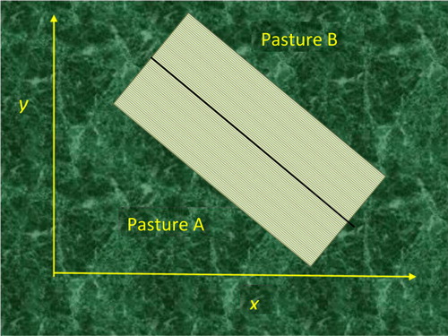
A rectangular paddock at the farm located at DPI Hamilton in Victoria was divided into two pastures, ryegrass and plantain, using the experimental plan in Figure 9. The paddock location and dimensions were subject to coordinate transformation to allow computations as multiple rows in the x-dimension for averaging results (as described previously). The dividing line between paddocks was open and without fencing, in order to allow the sheep to move freely between both paddocks. The sheep are known to identify the pasture types visually (i.e. random feeding explorations during a settling period was not a significant factor). The proportion of sheep in each paddock was calculated for each of three geometrical cases: dividing boundary at current level, for boundary offset δ = 0, then offset of δ = -6 m and finally offset of δ = -10 m. The reason for this was to address the uncertainty in position of the boundary relative to the error in GPS measurement data. The GPS units on the sheep were supplied by Alana Technology and nominally rated, with an error of 6.3 m according to device specifications. The effect of this sensor precision was to produce a fuzzy boundary between paddocks and therefore introduced a degree of spatial uncertainty in hypothesis testing.

Figure 9. Paddock orientation relative to the global coordinate frame, where Pastures A and B share a common boundary, and represent ryegrass and plantain, respectively (cf. Figure 3 with sheep locations and contextual information from Google Earth). Geometric transformations involving translation and rotation can be applied to align paddock boundaries to be parallel to the global reference frame.

A total of n = 99,849 locations were logged by the GPS for the individual sheep in the flock, over two paddocks, denoted A and B (for ryegrass and plantain, respectively), under the different offset scenarios. For zero offset, sheep preferring ryegrass represented a high proportion at p = 0.90 for los = 0.05 (two-tail). For offset of 6 m (at the expense of the ryegrass boundary), sheep preference in favour of ryegrass represented p = 0.79, and for offset of 10 m, it was p = 0.64. Since an offset of 6 m corresponded with the GPS uncertainty, it was concluded that the feeding preference experiments suggested that ryegrass was the preferred pasture, with approximately 73 ± 1% preference rating for the H₀, taking into account statistical significance of los = 0.05 for the estimated proportion, and including spatial uncertainty in the GPS locations. Using the test for comparing population means produced a z value, z = 429 (cf. z_crit = 1.645), which was highly significant at the same los level.

The last experiment was a methodology study and was noteworthy for its incorporation of statistical design principles, including testing the null hypothesis of no significant difference, together with quantification of spatial uncertainty at the boundary.

5. Summary and conclusions

The use of geovisual analytics provides a means of coping with the real-world problem of information overload by providing a decision support aid for human perceptions of important features in the data. Information processing and visualisation may expose data groupings, or clustering effects, not easily gleaned from numerous data tables and matrices, and also enables instant viewing of trend data. One issue confronting farmers is that the daily load of natural excreta of livestock adds to the N emissions affecting the local environment. Farmers in New Zealand require information on N losses in order to reduce emissions to meet local and international standards.

Geovisual analytics can provide information on animal behaviour and data for models used for estimating the quantity of N emissions from grazing animals. Moreover, data on N loads provide inputs to N recycling optimisation models for fertiliser allocation. Analysis based on data visualisation and feature extraction showed that urine and faecal excreta were not randomly distributed, but were highly localised and separated, and can be mapped to identify areas of significant environmental impact. Where behaviour can be predicted, or known through local knowledge, targeting and mitigation may become a cost-effective strategy. Within the context of geovisual analytics, an ABM can provide preliminary screening for the identification and localisation of clusters around excretion sites, and also identification of gathering sites on both sides of the boundary between the two pastures used to test feeding preferences. The agent-based approach also produces data visualisation to add support to the numerical analysis that was provided by statistical methods.

Another application of the geovisual analytic approach was the determination of animal feeding preferences using GPS data, including incorporation of an estimate of sensor precision. A statistical method was developed to compare sheep feeding preferences between two pastures using satellite tracking under conditions of spatial uncertainty. Under the current experimental conditions, the methodology revealed that ryegrass was the preferred pasture over plantain for 73% of sheep in the test.

References

- Andersson, M., J. Gudmundsson, P. Laube, and T. Wolle. 2008. “Reporting Leaders and Followers among Trajectories of Moving Point Objects.” GeoInformatica 12 (4): 497–528. doi:10.1007/s10707-007-0037-9
- Benke, K. K., and L. R. Benke. 2013. “Experiments in Optimal Spatial Segmentation of Local Regions Using Categorical and Quantitative Data.” Applied Spatial Analysis and Policy 6 (3): 185–208. doi:10.1007/s12061-012-9078-z
- Benke, K. K., and C. Pelizaro. 2010. “A Spatial-statistical Approach to the Visualisation of Uncertainty in Land Suitability Analysis.” Journal of Spatial Science 55 (2): 257–272. doi:10.1080/14498596.2010.521975
- Benke, K. K., C. J. Pettit, and K. E. Lowell. 2011. “Visualisation of Spatial Uncertainty in Hydrological Modelling.” Journal of Spatial Science 56 (1): 73–88. doi:10.1080/14498596.2011.567412
- Benke, K. K., F. Sheth, K. Betteridge, C. J. Pettit, and J.-P. Aurambout. 2012. “A Geo-visual Analytics Approach to Biological Shepherding: Modelling Animal Movements and Impacts.” ISPRS Annals of the Photogrammetry, Remote Sensing and Spatial Information Sciences, Vol. I-2, 2012 XXII ISPRS Congress, Melbourne, Australia, August 25–September 1.
- Betteridge, K. 2010. “Seminar on Logging and Data Distribution of Animal Urination and Defecation at Lake Taupo, New Zealand.” Paper presented at DPI Ellinbank, Victoria, July 8.
- Betteridge, K., D. Costall, S. Balladur, M. Upsdell, and K. Umemura. 2010. “Urine Distribution and Grazing Behaviour of Female Sheep and Cattle Grazing a Steep New Zealand Hill Pasture.” Animal Production Science 50 (6): 624–629. doi:10.1071/AN09201
- Betteridge, K., F. Li, D. Costall, A. Roberts, W. Catto, A. Richardson, and J. Gates. 2011. “Targeting DCD at Critical Source Areas as a Nitrogen Mitigation Strategy for Hill Country Farmers.” In Adding to the Knowledge Base for the Nutrient Manager, edited by L. D. Currie and C. L. Christensen, 13. Palmerston North, New Zealand: Fertilizer and Lime Research Centre, Massey University. http://flrc.massey.ac.nz/publications.html.
- Brown, D. G., R. Riolo, D. T. Robinson, M. North, and W. Rand. 2005. “Spatial Process and Data Models: Toward Integration of Agent-based Models and GIS.” Journal of Geographical Systems 7 (1): 25–47. doi:10.1007/s10109-005-0148-5
- Djordjevic, B., J. Gudmundsson, A. Pham, and T. Wolle. 2008. Detecting Regular Visit Patterns. Proceedings of 16th ESA 344–355.
- Freund, J. E. 1998. Mathematical Statistics. New York: Prentice Hall.
- Gudmundsson, J., P. Laube, and T. Wolle. 2008. Movement Patterns in Spatio-temporal Data. In Encyclopedia of GIS, edited by S. Shekhar, and H. Xiong, 726–732. New York: Springer.
- Johnson, R. A. 2007. Advanced Euclidean Geometry. New York: Dover Publications.
- Kantardzie, M. 2003. Data Mining: Concepts, Models, Methods, and Algorithms. New York: IEEE Press.
- Kreveld, M. van, B. Speckmann, and J. Gudmundsson. 2007. “Efficient Detection of Motion Patterns in Spatio-temporal Data Sets.” GeoInformatica 11 (2): 195–215. doi:10.1007/s10707-006-0002-z
- Laube, P., and T. Dennis. 2006. “Exploratory Analysis of Movement Trajectories.” GeoCart 2006, National Cartographic Conference, September 4–6, Auckland, NZ.
- Mayer, D. G., T. M. Davison, M. R. McGowan, B. A. Young, A. L. Matschoss, P. J. Goodwin, N. N. Johnson, and J. B. Gaughan. 1999. “Extent and Economic Effect of Heat Loads on Dairy Cattle Production in Australia.” Australian Veterinary Journal 77 (12): 804–808. doi:10.1111/j.1751-0813.1999.tb12950.x
- Mucherino, A., P. Papajoirgji, and P. Pardalos. 2009. Data Mining in Agriculture. Berlin: Springer.
- Silanikove, N., 2000. “Effects of Heat Stress on the Welfare of Extensively Managed Domestic Ruminants.” Livestock Production Science 67 (1–2): 1–18. doi:10.1016/S0301-6226(00)00162-7
- Singh, A. 1989. “Review Article Digital Change Detection Techniques Using Remotely-sensed Data.” International Journal of Remote Sensing 10 (6): 989–1003. doi:10.1080/01431168908903939
- Sposito, V., K. Benke, C. Pelizaro, and R. Wyatt. 2010. “Adaptation to Climate Change in Regional Australia: A Decision-making Framework for Modelling Policy for Rural Production.” Geography Compass 4 (4): 335–354. doi:10.1111/j.1749-8198.2009.00307.x
- Tang, W., and D. A. Bennett. 2010. “Agent-based Modeling of Animal Movement: A Review Agent-based Modeling of Animal Movement: A Review.” Geography Compass 4 (7): 682–700. doi:10.1111/j.1749-8198.2010.00337.x
- Thomas, G. B., and R. L. Finney. 1998. Calculus and Analytic Geometry. Reading, MA: Addison-Wesley.
- Wilensky, U. 1999. NetLogo. Center for Connected Learning and Computer-based Modeling. Evanston, IL: Northwestern University.