Spatiotemporal reflectance blending in a wetland environment

Abstract

To understand the mechanism of wetland cover change with both moderate spatial resolution and high temporal frequency, this research evaluates the applicability of a spatiotemporal reflectance blending model in the Poyang Lake area, China, using 9 time-series Landsat-5 Thematic Mapper images and 18 time-series Terra Moderate Resolution Imaging Spectroradiometer images acquired between July 2004 and November 2005. The customized blending model was developed based on the enhanced spatial and temporal adaptive reflectance fusion model (ESTARFM). Reflectance of the moderate-resolution image pixels on the target dates can be predicted more accurately by the proposed customized model than the original ESTARFM. Water level on the input image acquisition dates strongly affected the accuracy of the blended reflectance. It was found that either of the image sets used as prior or posterior inputs are required when the difference of water level between the prior or posterior date and target date at Poyang Hydrological Station is <2.68 m to achieve blending accuracy with a mean average absolute difference of 4% between the observed and blended reflectance in all spectral bands.

Keywords:

• time-series
• blending model
• spatial-temporal reflectance
• multi-sensor
• Landsat TM
• MODIS

1. Introduction

It is widely recognized that wetlands are one of the most significant natural resources biologically and biochemically, in spite of their small coverage of the global land surface (6% or 9 × 10⁶ km²) (Erwin 2009). Wetlands perform a variety of functions including controlling floods, recharging groundwater, improving water quality, mitigating erosion, retaining nutrients, emitting methane gas, and providing unique habitats for flora and fauna (Henderson and Lewis 2008). Despite several wetland and biodiversity conservation projects around the world, more than half of global wetlands have been lost in the last century, mainly because of human activities and global climate change (Cronk and Fennessy 2001). The functions of wetlands can be affected by their location and hydrologic periods, which can be altered by wetland loss and alternation (Lang et al. 2008). Therefore, it is clearly essential to monitor hydrologic patterns in wetland ecosystems such as inundation and soil moisture changes, both spatially and temporally, toward better understanding of the causal factors of wetland ecosystem change.

Remote sensing is an important component of Digital Earth techniques (Goodchild 2008). Earth observation satellites greatly promote remote sensing applications ranging from scientific research to practical and operational use (Guo et al. 2012). As robust and economical tools, optical satellite remote sensing has been used to monitor wetlands over large and inaccessible areas with high efficiency and accuracy (Davranche, Lefebvre, and Poulin 2010). In particular, multitemporal satellite imagery has aided in understanding of the changes in water and land cover in wetland ecosystems. Previous studies have used moderate spatial resolution imagery primarily for monitoring spatial details of wetland cover changes at local scale (Munyati 2000) and coarse spatial resolution imagery for monitoring temporal dynamics of water and land cover changes in wetlands at regional and global scales (Hui et al. 2008). However, the trade-off between spatial resolution and revisiting intervals of satellite remote sensors has limited deeper investigation of the mechanism of wetland cover change at both moderate spatial resolution and high temporal frequency (Zhao, Stein, and Chen 2011).

To overcome this difficulty, several techniques have been developed to integrate two sources of optical remotely sensed imagery with varying spatial resolution and temporal frequency. The enhanced spatial and temporal adaptive reflectance model (ESTARFM; Zhu et al. 2010) is one of the blending models that produce synthetic, moderate spatial resolution data at the time intervals of coarse spatial resolution imagery. ESTARFM has an advantage over the original spatial and temporal adaptive reflectance model (STARFM; Gao et al. 2006) in blending reflectance in pixels of heterogeneous land cover that are very common in wetlands. Nevertheless, there has been a lack of studies incorporating spatiotemporal reflectance blending to monitor wetlands where land and water cover change dramatically throughout the year. Quite some previous researches have modeled wetland cover changes in the Poyang Lake area using multi-temporal optical remotely sensed imagery. Time-series remotely sensed images with moderate spatial resolution, such as the Landsat Thematic Mapper (TM) data, have been used to understand the spatial details of seasonal and interannual land and water cover changes (Dronova, Gong, and Ling 2011; Gong et al. 2010; Hui et al. 2008). Researches using time-series remotely sensed data with coarse spatial resolution, such as Terra MODIS data, have focused on the monitoring of temporal dynamics in lake water fluctuations (Feng et al. 2012; Cui, Wu, and Liu 2009). Although it is critically important to monitor the study area at both moderate spatial resolution and high temporal frequency for an improved understanding of the mechanism in rapid land and water cover changes, there have been a limited number of researches using multiple sources of time-series remotely sensed data with different spatial and temporal resolutions (Michishita et al. 2012). The previous study applied the spectral unmixing method to derive time-series characteristics of land cover fractions separately from the TM and MODIS at the intervals of TM image observations (Michishita et al. 2012), while this study blended moderate spatial resolution images to monitor the spatial–temporal dynamics of different land cover types with high temporal frequency.

As a continued research of Zhu et al. (2010), this research evaluates the applicability of spatiotemporal reflectance blending model in monitoring wetland cover changes, taking the Poyang Lake as an example, using time-series Landsat-5 TM and MODIS images. Therefore, this research is designed to compare observed TM images and blended images generated for the TM observation dates by blending model, as a preliminary study to generate dense time-series reflectance images with moderate spatial resolution. Three specific research objectives are: (1) to customize an existing reflectance blending model to address problem with MODIS images observed on TM image acquisition dates across the study area; (2) to assess the influence of TM image observation intervals and water level differences between prior or posterior and target dates on blending accuracy; and (3) to select input image combinations that achieve optimum agreement between observed and blended reflectance.

2. ESTARFM

ESTARFM (Zhu et al. 2010) requires two pairs of moderate and coarse spatial resolution images (hereafter, moderate-resolution, and coarse-resolution images) on prior and posterior dates and one coarse-resolution image on the target date. Following assumptions were made in the development of ESTARFM:

1. The proportions of land cover types contained in the mixed pixels of coarse-resolution data do not change during a short-time period.

2. The reflectance linearly changes during a short-time period.

3. The proportion of each end-member and the change rate of the surface reflectance for each end-member are stable.

4. Similar pixels within one coarse-resolution data have the same conversion coefficients.

There are four major steps in the implementation of ESTARFM:

1. Two moderate-resolution images are individually used to search for pixels similar to the central pixel in a moving window. The ith neighboring pixel is selected as a similar pixel, if all the bands for the neighboring pixel satisfy Equation (1) for the prior moderate-resolution image and Equation (2) for the posterior moderate-resolution image:

   (1)
   (2)
   where M denotes the moderate-resolution reflectance, x_i and y_i designate the location of the ith neighboring pixel, t_m and t_n are the acquisition dates of the prior and posterior moderation-resolution images, B denotes the spectral band, w is the moving window size, x_w/2 and y_w/2 designate the location of the central pixel, σ(M(t_m, B)) and σ(M(t_n, B)) denote standard deviations of reflectance for band B of prior and posterior moderate-resolution images in the moving window, and c is the estimated number of classes. The window size w is determined by the homogeneity of surface, with a smaller w when the regional landscape is more homogeneous. The two moderate-resolution images acquired at the prior and posterior dates were used to select similar pixels, and the intersection of their results was extracted to derive a final set of similar pixels.

2. The weights of all similar pixels (W_i) are determined by the correlation coefficient between moderate- and coarse-resolution data, as a measure of spectral similarity and geographic distance between the target and similar pixels. Details of the calculation of spectral similarity and geographic distance are found in Zhu et al. (2010).

3. Conversion coefficients (V_i) are calculated from the surface reflectance of moderate- and coarse-resolution data through linear regression. The slope of the linear regression model corresponds to V_i. Linear regression models were applied to the moderate- and coarse-resolution reflectance of similar pixels within the same coarse-resolution pixel to obtain the conversion coefficients.

4. Reflectance of the moderate-resolution image on the target date (t_t) can be blended based on reflectance of the moderate-resolution images (M(x_w/2, y_w/2, t_m, B), M(x_w/2, y_w/2, t_n, B)) on the base dates (t_m, t_n), resampled reflectance of the coarse-resolution images (C(x_i, y_i, t_m, B), C(x_i, y_i, t_n, B)) on the baseline dates and resampled reflectance of the coarse-resolution image C(x_i, y_i, t_t, B) on t_t. Blended surface reflectance for band B at target pixel (x_w/2, y_w/2) on t_t utilizing two base image pairs on t_m and t_n (M_m(x_w/2, y_w/2, t_t, B) and M_n(x_w/2, y_w/2, t_t, B)) is calculated according to the Equations (3) and (4).

   (3)
   (4)
   Surface reflectance on t_t can be obtained by a weighted combination of the two prediction results above. The temporal weight for M_m(x_w/2, y_w/2, t_t, B), denoted by T_m, and for M_n(x_w/2, y_w/2, t_t, B), denoted by T_n, can be determined using the change magnitude calculated from the coarse-resolution images between t_m or t_n and t_t, as follows:
   (5)
   (6)
   The final blended reflectance of the moderate-resolution pixel on t_t (M(x_w/2, y_w/2, t_t, B)) is calculated as follows:
   (7)

3. Study area, data, and preprocessing

3.1. Study area

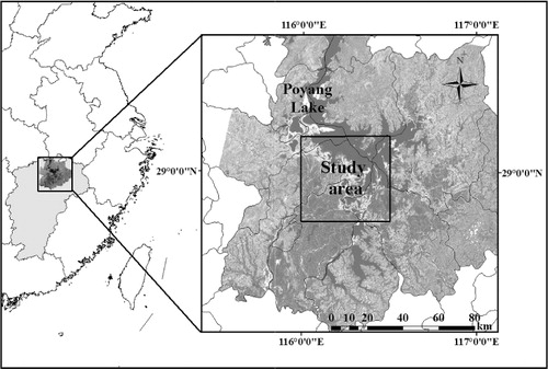
We chose a part of the Poyang Lake Nature Reserve (PLNR) in the northwest part of Poyang Lake in Jiangxi Province, China (116° 15′ E, 29° 00′ N) as our study area (Figure 1). Poyang Lake is the largest freshwater lake in China and experiences fluctuation of water level throughout the year with a minimum from December to February and a maximum from July to September. The extent of Poyang Lake varies from about 4000 km² in summer to <1000 km² in winter. The main sources of the water supply in the lake are its five main tributaries between March and June, and rain and the flood backflows from the Yangtze River between July and September (Guo et al. 2005).

Figure 1. Study area of Poyang Lake National Nature Reserve (PLNR), China.

Wetlands in the PLNR are important food resources for wintering migratory birds, particularly cranes. For example, 98% of the global population of Siberian Cranes stayed in the area during winter of 2001 (Higuchi et al. 2004). Wetlands in the area have also been one of the major endemic sites of schistosomiasis in China because they create favorable habitats for intermediate host snails (Zhou et al. 2005). In the past few decades, human activities and regional climate change have altered water and land cover in this area, consequently producing heavy sedimentation, lake shrinkage, change of inundation trend, biodiversity loss, and re-emergence of schistosomiasis (Fang et al. 2006).

3.2. Data and preprocessing

We used nine time-series Landsat-5 TM Level-1b products (30 m spatial resolution, six spectral bands except for the thermal band) and 18 time-series Terra MODIS daily surface reflectance (MOD09GA) products (480 m spatial resolution, seven spectral bands). These products were observed from July 2004 through November 2005 and are detailed in Table 1. MODIS products acquired on the TM image acquisition dates were not used because of a large unobserved area and striped strong noise patterns around the unobserved area in the scenes. The blending model incorporated in this research thus required the customization based on the ESTARFM to use the MODIS products acquired on prior and posterior dates of TM product observation dates, due to this unique condition of MODIS image acquisition across the study area.

Table 1. Acquisition dates of the input Landsat-5 TM and Terra MODIS images for the customized model.

			MODIS
Year	Code	TM	Prior	Posterior
2004	A, a	24 July	22 July	27 July
	B, b	28 October	27 October	29 October
	C, c	29 November	28 November	2 December
	D, d	15 December	12 December	16 December
2005	E, e	5 March	22 February	6 March
	F, f	12 August	8 August	17 August
	G, g	13 September	12 September	16 September
	H, h	29 September	21 September	30 September
	I, i	31 October	30 October	21 November

We georegistered the TM image of 28 October 2004 by registering the image to the map published by the Editing Committee of Jiangxi Map Collection (2008). A first-order polynomial fit using 24 ground control points (GCPs) applied to the base image produced an average root mean square error (RMSE) of 0.25 pixels. Image-to-image registration between the georegistered TM image and the other eight TM images was done using 30 GCPs and a first-order polynomial fit, producing an average RMSE <0.25 pixels. In both registration processes, nearest-neighbor resampling was applied to preserve the original brightness values. Surface reflectance was derived from the geometrically corrected TM images using a radiative transfer model implemented in Atmospheric Correction Now (ImSpec LLC 2008) software. We used six TM bands excluding the thermal band.

By contrast, only map re-projection and image resampling to the TM spatial resolution (30 m) were performed on the MODIS images. There are two reasons for this: (1) the MOD09GA products were geometrically accurate compared to the TM data; and (2) the MOD09GA products had already been atmospherically corrected. We used six MODIS bands in the products except for Band 5. In bandwidth of the spectral bands, TM Band 1 corresponds to MODIS Band 3 (blue), TM Band 2 to MODIS Band 4 (green), TM Band 3 to MODIS Band 1 (red), TM Band 4 to MODIS Band 2 (near infrared: NIR), TM Band 5 to MODIS Band 6 (shorter portion of shortwave infrared: S-SWIR), and TM Band 7 to MODIS Band 7 (longer portion of shortwave infrared: L-SWIR).

Water level records at the Poyang Hydrological Station (PHS) from the study period were also collected to investigate criteria for the choice of input images for the reflectance blending model; this was done by comparing the average absolute difference (AAD) between the blended and the observed reflectance with water level, which corresponded to the smaller absolute difference of water level between prior or posterior date and target date of TM image observations. Water level was recorded at 8:00 am every day.

4. Method

The analysis consisted of three parts. First, a spatiotemporal reflectance blending model accounting for the unique condition of the MODIS image observations across the study area, which has been mentioned in the section of 3.2, was developed through customization of the original ESTARFM. Next, we assessed the influence of TM image observation intervals and water level difference between prior or posterior dates and target date on the accuracy of the blended reflectance. Finally, the input image combination achieving maximum agreement between observed and blended reflectance was selected for each target date.

4.1. Customization of ESTARFM

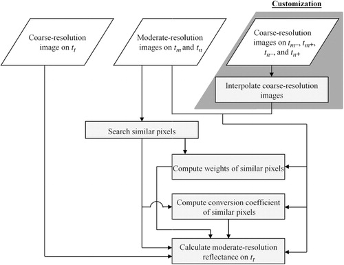
To deal with the unique observation condition of MODIS images across the study area on the TM image observation dates, we customized the ESTARFM as shown in Figure 2. The customized blending model added temporal weight interpolation of the MODIS images on the prior and posterior dates of TM image acquisition date, before the first step of the ESTARFM (explained in Section 2), to generate MODIS images on the observation dates of TM images. Thus, the customized model required two TM images on the prior and posterior dates of the target date; two MODIS images on the prior and posterior dates of each TM observation date, which in summary including four MODSI images; and one MODIS image on the target date. MODIS reflectance for the observation dates of the prior and posterior TM images (C_m, C_n) were interpolated using the MODIS images observed before and after each TM image observation dates as follows:

(8)

(9)

Figure 2. Flowchart of customized blending model based on ESTARFM. t_t refers to target date of blended reflectance image, t_m and t_n refers to acquisition dates of prior and posterior TM images, t_m − and t_m + refers to acquisition dates of prior and posterior MODIS images for prior TM image, and t_n − and t_n + refers to acquisition dates of prior and posterior MODIS images for posterior TM image.

where t_m− and t_m + refer to acquisition dates of the prior and posterior MODIS images for the prior TM input image, t_n− and t_n + refer to acquisition dates of the prior and posterior MODIS images for the posterior TM input image, C_m− and C_m + to MODIS reflectance on the prior and posterior dates for the prior TM input image, C_n− and C_n + to MODIS reflectance on the prior and posterior dates for the posterior TM input image, respectively. We implemented the blending process with the ESTARFM followed by the temporal interpolation of the MODIS images. Theoretically, only one MODIS image is necessary as the input image for the target date. In order to compare the blended and the observed reflectance, however, the input MODIS image for the target date in our study was also interpolated by two MODIS images on the prior and posterior dates of target date of observed TM images as shown in Equation 6. In the calculation of blended reflectance, all input control parameters were set identical to those in Zhu et al. (2010).

Modeling accuracy was assessed through comparison of the blended reflectance from the blending models and observed TM reflectance for 28 October 2004. To examine the difference of ESTARFM and our customized model, we used AAD and average difference (AD) between observed TM reflectance and blended reflectance of moderate-resolution images, from both the models. Compared with our customized model, two prior and posterior TM images, two MODIS images on the closest dates of TM observation dates, and one MODIS image on target date were used as input data for ESTARFM. AAD was used to quantify errors of blended reflectance, while AD was used to examine the reasons of errors (overestimation indicated by positive value, underestimation indicated by negative value, and same degrees of overestimation and underestimation by value close to zero).

4.2. Investigation of factors in input images influencing blending accuracy

It was demonstrated in previous studies that agreement between observed and blended reflectance is dependent on the combination of input image sets (Walker et al. 2012; Watts et al. 2011). This research investigated which factors in the input images influenced agreement between observed reflectance and blended reflectance from the customized model. We focused on two factors: (1) a shorter interval of TM image observations between prior or posterior date and target date; and (2) smaller absolute difference of water level at PHS between prior or posterior date and target date of TM image observations. All possible combinations of the TM and MODIS image sets in chronological order were used as the prior and posterior inputs, to blend reflectance for the seven target TM observation dates (28 October, 29 November, and 15 December in 2004 and 5 March, 12 August, 13 September and 29 September in 2005). For each blended image, AAD was calculated between the observed and blended reflectance. We analyzed the relationships between AAD for each spectral band and the two aforementioned factors, based on the adjusted correlation coefficient (adjusted R ² ). Adjusted R ² between the factors and AAD was calculated, not only for the entire study period but also for each of four seasons (March–May, spring; June–August, summer; September–November, fall; and December–February, winter).

4.3. Selection of optimal input image set combination for reflectance blending

The combination of the input image sets achieving the greatest agreement between observed and blended reflectance was selected as the optimal combination for each target date. Agreement was evaluated based on mean values of AAD between observed and blended reflectance for each spectral band. We compared AAD and AD for the optimal blended moderate-resolution images on the target dates during different seasons, to examine their temporal variations. To examine the difference of agreement between observed and blended reflectance for varying land cover types, AAD and AD were calculated not only for the entire study area, but also for land and water bodies separately, using the observed and blended images of 28 October 2004. In the calculation, we applied image masks built by thresholding of normalized difference vegetation index (NDVI) images derived from the observed reflectance image. An NDVI threshold value of 0.2 was determined empirically in our preliminary analysis.

5. Results

5.1. Customization of ESTARFM

Figure 3 shows false color images of observed TM reflectance and blended reflectance predicted by the customized blending model and ESTARFM, acquired on 28 October 2004. For the customized model, TM images acquired on 24 July and 29 November 2004 were used as the input moderate-resolution images and MODIS images acquired on 22 and 27 July, 27 and 29 October, 28 November, and 2 December 2004 were used as the input coarse-resolution images. For the ESTARFM, TM images acquired on 24 July and 29 November 2004 were used as the input moderate-resolution images, and MODIS images acquired on 22 July, 29 October, and 28 November 2004 were used as the input coarse-resolution images. The green, red, and NIR bands were assigned to blue, green, and red in the images along the top row; and the blue, S-SWIR, and L-SWIR bands were assigned to blue, green, and red in the images along the bottom row.

Figure 3. False color images of observed and blended reflectance: observed TM reflectance (a and d); blended reflectance predicted by customized model (b and e); and blended reflectance from ESTARFM for 28 October 2004 (c and f). Green, red, and near infrared (NIR) bands were assigned to blue, green, and red in images along top row (a–c), and blue, shorter portion of shortwave infrared (S-SWIR), and longer portion of shortwave infrared (L-SWIR) bands were assigned to blue, green, and red in images along bottom row (d–f).

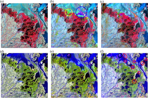
The images predicted by the customized model (Figure 3b and 3e) and ESTARFM (Figure 3c and 3f) were very similar to the actual images (Figure 3a and 3d) in most parts of the study area. We can see the spatial distributions of large and small patches of water and land cover in the moderate-resolution blended reflectance images generated by both models. However, both models generated smaller reflectance in vegetated areas than the observed reflectance from the NIR band, leading to the bluish false color images of the green, red, and NIR bands (Figure 3b and 3c). In addition, both models failed to blend the reflectance correctly in transition zones from sand and mud to water bodies. For example, the customized model underestimated green reflectance in the light green area within the yellow circle, and red reflectance in the magenta area within the blue circle of Figure 3b. ESTARFM overestimated L-SWIR reflectance in the magenta areas within the red circles of Figure 3f, and both models overestimated this band's reflectance in the water bodies within the black circles of Figure 3e and 3f.

AAD and AD values between the observed reflectance and blended reflectance generated by both models for 28 October 2004 are listed in Table 2. In both models, errors indicated by AAD were generally larger in the spectral bands with longer wavelengths (NIR, S-SWIR, and L-SWIR) than in the spectral bands with shorter wavelengths (red, green, and blue). As indicated by AAD, the prediction of the customized blending model was slightly more accurate than ESTARFM in all bands. In particular, the customized model improved the blending accuracy over ESTARFM most significantly in the S-SWIR band (AAD = 3.65% reflectance for the customized model and 4.37% reflectance for ESTARFM). For the customized model, small overestimation of blended reflectance was found in the green (AAD = 1.50% reflectance, AD = 0.85% reflectance) and red bands (AAD = 1.55% reflectance, AD = 0.41% reflectance). Underestimation of the customized model was evident in the NIR band (AAD = 3.52% reflectance, AD = −0.84% reflectance). The large errors in the S-SWIR (AAD = 3.65% reflectance) and L-SWIR (AAD = 3.00% reflectance) bands were resulted from both a noticeable degree of both overestimation and underestimation which were explained by a value of AD close to zero (0.08% reflectance for the S-SWIR band and −0.10% reflectance for the L-SWIR band). ESTARFM overestimated the blended reflectance slightly in the red band (AAD = 1.65% reflectance, AD = 0.54% reflectance) and significantly in the S-SWIR (AAD = 4.37% reflectance, AD = 1.27% reflectance) and L-SWIR (AAD = 3.26% reflectance, AD = 0.87% reflectance) bands. Underestimation by ESTARFM was noticeable in the NIR band (AAD = 3.78% reflectance, AD = −0.49% reflectance).

Table 2. AAD and AD between observed reflectance and blended reflectance from the customized model and ESTARFM for 28 October 2004.

	AAD, %reflectance		AD, %reflectance
Band	Customized model	ESTARFM	Customized model	ESTARFM
Blue	0.92	1.08	0.04	0.05
Green	1.50	1.75	0.85	0.30
Red	1.55	1.65	0.41	0.54
NIR	3.52	3.78	−0.84	−0.49
S-SWIR	3.65	4.37	0.08	1.27
L-SWIR	3.00	3.26	−0.10	0.87

The above findings prove that the customized blending model is capable of predicting reflectance images with sufficient accuracy to map the wetland environment in the study area, accounting for the MODIS image observation problem on the TM image observation dates.

5.2. Investigation of factors in input images influencing blending accuracy

Table 3 summarizes the adjusted R ² between factors in the input images and AAD between observed and blended reflectance. Adjusted R ² was calculated using reflectance from a total of 84 images, generated by the customized model with all possible input combinations in chronological order (16 combinations for spring, 15 for summer, 38 for fall, and 15 for winter).

Table 3. Adjusted correlation coefficient (adjusted R ² ) between factors in input images and AAD between observed and blended reflectance.

	Band
Season	Blue	Green	Red	NIR	S-SWIR	L-SWIR
Shorter image observation interval
All	0.02	0.00	0.10	0.12	0.33	0.38
Spring	0.08	0.00	0.35	0.43	0.27	0.23
Summer	0.00	0.01	0.61	0.55	0.51	0.19
Fall	0.02	0.00	0.10	0.18	0.20	0.22
Winter	0.64	0.26	0.56	0.71	0.81	0.87
Smaller absolute water level difference between prior or posterior dates and target dates
All	0.16	0.14	0.40	0.53	0.64	0.61
Spring	0.46	0.34	0.24	0.19	0.34	0.37
Summer	0.62	0.00	0.00	0.38	0.66	0.67
Fall	0.23	0.30	0.54	0.73	0.58	0.51
Winter	0.69	0.41	0.77	0.94	0.92	0.94

Although the shorter image observation interval (Table 3) did not show strong correlation with AAD calculated across the whole season, it achieved a high adjusted R ² for the spectral bands with longer wavelengths in winter (0.71 for NIR, 0.81 for S-SWIR, and 0.87 for L-SWIR). It also had a moderate adjusted R ² for the red (0.61) and NIR bands (0.55) in summer and for the blue (0.64) and red bands (0.56) in winter. Adjusted R ² for all spectral bands remained low in the whole season, spring, and fall. The green band had very low adjusted R ² in all seasons. These results suggest that the shorter observation interval is an important factor to accurately generate the reflectance images in winter when the water level in Poyang Lake does not change much. In addition, the low adjusted R ² between shorter observation interval and AAD in spring and fall might be caused by land cover changes between prior and target dates and/or target and posterior dates as a result of rapidly increasing or decreasing water level in these periods. This resulted in consistently low AAD with varying shorter observation intervals.

The smaller absolute difference of water level (Table 3) showed moderate correlation with AAD calculated across the whole season for the NIR (0.53), S-SWIR (0.64), and L-SWIR bands (0.61). A high adjusted R ² was obtained for the NIR band (0.73) in fall, and for the red (0.77), NIR (0.94), S-SWIR (0.92), and L-SWIR (0.94) bands in winter. It also had a moderate adjusted R ² for the blue (0.62), S-SWIR (0.66), and L-SWIR (0.67) bands in summer, for the red (0.54), S-SWIR (0.58), and L-SWIR (0.51) bands in fall, and for the blue band (0.69) in winter. As seen in the comparison between the shorter image observation interval and AAD of reflectance, low adjusted R ² was obtained for the green band in all seasons. Adjusted R ² for all spectral bands was low in spring, possibly because the reflectance in the pixels of the shallow water bodies caused by the rapid submergence of sand, mud, and vegetated wetlands on the target date could not be generated accurately from the prior images, containing sand, mud, and vegetated wetlands, and posterior images, containing deep water bodies.

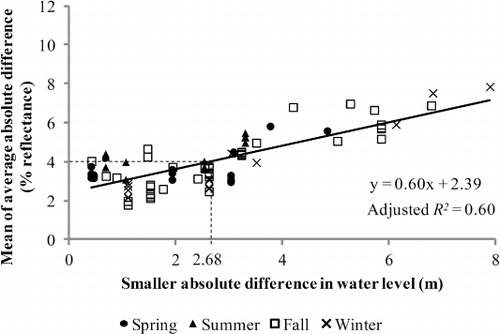
Figure 4 displays the relationship of the mean values of AAD between observed and blended spectra in all bands with smaller absolute difference of water level between prior or posterior dates and target dates. Mean values of AAD between observed and blended spectra increased linearly as the smaller absolute difference of water level between prior or posterior dates and target dates increased. Mean values of AAD in all bands indicate that either the prior or posterior input TM image is necessary when the water level difference between the prior or posterior date and target date at PHS is <2.68 m, to achieve a mean AAD of 4% reflectance between the observed and blended reflectance in all spectral bands. This finding implies the importance of referring water level record to select appropriate input TM and MODIS images, for the accurate blending of moderate-resolution reflectance images in wetlands.

Figure 4. Relationship of the mean values of AAD between observed and blended spectra in all bands with smaller absolute difference of water level between prior or posterior dates and target dates.

The investigation in this section revealed that the accuracy of the blending reflectance was more directly affected by water level difference between input image acquisition dates than intervals of the acquisition dates when a study area included large areas of dynamic water bodies, such as Poyang Lake in the study area.

5.3. Selection of optimal input image set combination for reflectance blending

Table 4 shows agreement between observed and blended reflectance generated with the combination of input image sets generating smallest mean values of AAD for all spectral bands. AAD and AD are summarized in Table 4a and b, respectively. Each three-letter code in the input combinations corresponds to the observation dates in Table 1. The first and third lowercase letters refer to the prior and posterior dates, respectively, and the second uppercase letter to the target date. Therefore, one TM image and two MODIS images were used on the dates denoted by lowercase letters, whereas two MODIS images were used on dates denoted by uppercase letters.

Table 4. Agreement between observed and blended reflectance with combination of input image sets achieving smallest mean values of AAD for all spectral bands: (a) AAD, (b) AD.

(a)
Target date				AAD,% reflectance
Year	Date	Combination	Area	Blue	Green	Red	NIR	S-SWIR	L-SWIR	Mean: all
2004	28 October	aBc	Whole	0.92	1.50	1.55	3.52	3.65	3.00	2.36
			Land	0.86	1.48	1.42	4.16	4.14	3.31	2.56
			Water	1.04	1.56	1.83	2.27	2.69	2.40	1.96
	29 November	bCd	Whole	0.90	1.30	1.36	2.11	2.79	2.25	1.78
	15 December	cDh	Whole	1.39	1.52	1.58	2.25	3.37	2.86	2.16
2005	5 March	dEg	Whole	2.33	2.15	1.88	3.48	4.26	3.51	2.94
	12 August	aFg	Whole	2.82	3.09	2.51	5.26	2.94	1.76	3.06
	13 September	fGh	Whole	3.65	3.65	2.98	5.36	3.84	2.56	3.67
	29 September	aHi	Whole	1.60	1.56	2.23	4.09	3.17	2.90	2.59
(b)
Target date		AD,% reflectance
Year	Date	Area	Blue	Green	Red	NIR	S-SWIR	L-SWIR
2004	28 October	Whole	0.04	0.85	0.41	−0.84	0.08	−0.10
		Land	−0.08	0.78	0.30	−1.65	−0.24	−0.30
		Water	0.28	0.99	0.63	0.74	0.71	0.30
	29 November	Whole	0.07	−0.58	−0.16	−0.31	0.05	0.00
	15 December	Whole	−0.81	−0.01	0.17	0.22	−0.74	−1.18
2005	5 March	Whole	2.05	1.26	0.31	−0.66	−0.92	0.06
	12 August	Whole	2.24	2.34	1.45	1.94	0.31	−0.04
	13 September	Whole	3.03	1.55	1.49	1.35	2.30	1.29
	29 September	Whole	0.08	−0.32	0.21	−1.38	0.28	−1.22

The blended reflectance generated by the customized blending model did not always have the smallest mean values of AAD for all spectral bands, when the combinations of input image sets used in the blending consisted of images acquired on the prior and posterior dates closest to the target dates (‘Combination’ column in Table 4a). Specifically, the sets of input images acquired on both prior and posterior dates closest to the target dates, manifested in three alphabets in a consecutive order (aBc, bCd, and fGh), achieved the strongest agreement (smallest mean values of AAD) in all possible combination of input image sets for 28 October and 29 November in 2004, and 13 September in 2005. In contrast, the smallest mean values of AAD were obtained by the input sets containing the images acquired on either prior or posterior dates closest to the target dates for the other target dates (15 December in 2004, 5 March, 12 August, and 29 September in 2005). The smallest mean value of AAD was smallest (1.78% reflectance) for 29 November in 2004 and largest (3.67% reflectance) for 13 September in 2005, when compared among all target dates.

The blending error of the customized model, indicated by AAD (Table 4a) and AD (Table 4b), varied among different target dates. Largest overestimation was found in the blended reflectance of all spectral bands for 13 September in 2005 (AAD = 3.65, 3.65, 2.98, 5.36, 3.84, and 2.56% reflectance, AD = 3.03, 1.55, 1.49, 1.35, 2.30, and 1.29% reflectance for blue, green, red, NIR, S-SWIR, and L-SWIR bands, respectively). The customized model underestimated the blended reflectance most significantly in the NIR band for 29 September in 2005 (AAD = 4.09% reflectance, AD = −1.38% reflectance), in S-SWIR band for 5 March in 2005 (AAD = 4.26% reflectance, AD = −0.92% reflectance), and in L-SWIR bands for 29 September in 2005 (AAD = 2.90% reflectance, AD = −1.22% reflectance). Other large overestimation was made in the blue and green bands for 5 March (AAD = 2.33 and 2.15% reflectance, AD = 2.05 and 1.26% reflectance, respectively) and in the three visible and NIR bands for 12 August in 2005 (AAD = 2.82, 3.09, 2.51, and 5.26% reflectance, AD = 2.24, 2.34, 1.45, and 1.94% reflectance for blue, green, red, and NIR bands, respectively). Large underestimation was also confirmed in the NIR band for 28 October in 2004 (AAD = 3.52% reflectance, AD = −0.84% reflectance), in the S-SWIR and L-SWIR bands for 15 December in 2004 (AAD = 3.37 and 2.86% reflectance, AD = −0.74 and −1.18% reflectance, respectively), and in the NIR band for 5 March in 2005 (AAD = 3.48% reflectance, AD = −0.66% reflectance). Other large errors, such as in the S-SWIR and L-SWIR bands for 28 October (AAD = 3.65 and 3.00% reflectance) and for 29 November in 2004 (AAD = 2.79 and 2.25% reflectance), in the L-SWIR band for 5 March in 2005 (AAD = 3.51% reflectance), in the S-SWIR band for 12 August in 2005 (AAD = 2.94%), and in the S-SWIR band for 29 September in 2005 (AAD = 3.17%), were caused by certain degrees of both overestimation and underestimation. These variations in AAD and AD for different target dates in every spectral band revealed the dependency of the blending accuracy on other potential factors in the input images except for image observation interval and water level. These possible factors influencing the accuracy of blended reflectance will be discussed in the next section.

AAD and AD for land and water bodies calculated from the observed and blended reflectance for 28 October in 2004 demonstrated their different characteristics. For both land and water bodies, there were larger errors, indicated by higher AAD, in the spectral bands with longer wavelengths (NIR, S-SWIR, and L-SWIR) than in the visible bands (blue, green, and red), but the differences of errors between the visible bands and bands with longer wavelengths were greater for land than for water bodies. The errors for land were slightly smaller than those for water bodies in the three visible bands, while the errors for land were greatly larger than those for water bodies in the three bands with longer wavelengths. In land, the customized model a little overestimated the blended reflectance in the green band (AAD = 1.48% reflectance, AD = 0.78% reflectance) and significantly underestimated the blended reflectance in the NIR band (AAD = 4.16% reflectance, AD = −1.65% reflectance). Large errors for the two SWIR bands (AAD = 4.14% and 3.31% reflectance for the S-SWIR and L-SWIR bands, respectively) were brought by both the overestimation and underestimation of the blended reflectance, although the underestimation was greater than the overestimation as explained by the negative AD (−0.24% reflectance for the S-SWIR band and −0.30% reflectance for the L-SWIR band). In water bodies, the blended reflectance was overestimated to a certain degree in green (AAD = 1.56% reflectance, AD = 0.99% reflectance), red (AAD = 1.83% reflectance, AD = 0.63% reflectance), NIR (AAD = 2.27% reflectance, AD = 0.74% reflectance) and S-SWIR (AAD = 2.69% reflectance, AD = 0.71% reflectance) bands. The error in the L-SWIR band (AAD = 2.40% reflectance) was brought by larger overestimation and smaller underestimation of the blended reflectance. Thus, pixels for land and those for water bodies showed different degrees of agreement between the observed and blended reflectance images among the spectral bands. These distinctive characteristics of reflectance blending in land and water bodies have not been investigated in previous research, and therefore they are the new findings in this study.

6. Discussion

The investigation on the applicability of the reflectance fusion models in this study revealed that the customized model can predict reflectance in the wetland environment of PLNR more accurately than the original ESTARFM. Water level on input image acquisition dates more directly affected the accuracy of the customized model than the intervals of the acquisition dates. This section focuses on other possible factors influencing the blending accuracy by the customized model.

The first potential factor influencing blending accuracy is cloud contamination in the input images. Table 4a and b demonstrated that the optimal blended reflectance images for 5 March, 12 August, and 13 September in 2005 had different characteristics in their errors, such as significant overestimation in the blue and green band for the three dates, in red band for 12 August and 13 September in 2005, and in the two SWIR bands for 13 September in 2005. All of these three optimal blended reflectance images were generated commonly using the two MODIS images for 13 September in 2005 observed on 12 and 16 September in 2005 (denoted by G and g in Table 1 and “Combination” column in Table 4a). In fact, the whole area in the MODIS reflectance image observed on 16 September in 2005 was covered with very thin clouds. As a result, the cloud contamination degraded the blending accuracy of the customized model.

Temporal weight interpolation of MODIS images to generate the coarse-resolution reflectance images for prior, posterior, and target date is the second potential factor of blending error. We utilized six input MODIS images (two for prior date, two for posterior date, and two for target date) to generate moderate-resolution reflectance images to compare with observed TM images. It may be the case that the customized model fails to select similar neighboring pixels and assign appropriate similarity weights and conversion coefficient for a target pixel in a moderate-resolution image, if unrealistic reflectance generated by the temporal interpolation was included in coarse-resolution pixels within a moving window. In consequence, the model generated more unrealistic reflectance in the blended images. Some areas of sand and mud (magenta area within the blue circle and the light green area within yellow circle in Figure 3b) contained differences between observed (Figure 3a) and blended reflectance possibly caused by the temporal weight interpolation of the MODIS reflectance, since the same area in the false color images generated by ESTARFM (Figure 3c) did not have noticeable differences from those of the observed images.

The rapid land cover changes that cannot be predicted precisely by input images might be the third factor influencing the modeling accuracy of not only the customized model but also the original ESTARFM. Both models can accurately blend the reflectance for a target date when they meet the four modeling assumptions described in Section 2. However, they cannot precisely blend the reflectance, if the land cover in the study area significantly changes during short periods of time beyond the modeling assumptions. For example, areas within the black circles commonly seen in Figure 3e and f were modeled as sand or mud by both models, but were water bodies in the observed image (Figure 3d).Thus, inaccurate reflectance could be predicted for a moderate-resolution pixel through the blending of two one-sided reflectance, if two one-sided reflectance in the same pixel had absolutely different spectral characteristics due to rapid and extensive land cover changes between the prior and target dates and/or the target and posterior dates, as implied in Zhu et al. (2010).

The fourth possible factor relates to the preprocessing of input images. This study used the Landsat-5 Level-1b products. The blending accuracy will increase if the effect of the bidirectional reflectance distribution function in the TM images is minimized, as Gao et al. (2006) pointed out. The accuracy can be improved if we use the TM input images atmospherically corrected with the Landsat Ecosystem Disturbance Adaptive Processing System (Masek et al. 2006), since MODIS products are atmospherically corrected using the same radiative transfer model.

This study suggests the difficulty of generating reflectance in areas with rapid and extensive land cover change between prior and target dates and between target and posterior dates. In order to increase the accuracy of the customized blending model particularly in the study area with rapid changing dynamic, refinement of the model is necessary, accounting for the factors above.

7. Conclusions

This research evaluated the applicability of a spatiotemporal reflectance blending model in monitoring wetland cover changes, using time-series Landsat-5 TM and Terra MODIS images acquired between July 2004 and November 2005 in PLNR. We customized the ESTARFM to account for the problems in the MODIS images acquired on the TM image observation dates by adding temporal weight interpolation of the MODIS images on the prior and posterior dates of TM image acquisition dates, and compared the observed TM reflectance and blended reflectance generated for the TM observation dates by the customized model.

Reflectance of moderate-resolution image pixels on the target dates could be predicted more accurately by the customized blending model than the original ESTARFM across the study area. Spatial distributions of large and small patches of water and land cover were captured by moderate-resolution blended reflectance images generated by the customized model. We found that water level on the input image acquisition dates affected accuracy of the blending reflectance more directly than did intervals of the input image acquisition dates. To achieve a mean AAD of 4% between the observed and blended reflectance in all spectral bands, either the prior or posterior input TM image observed when the water level difference between the prior or posterior date and target date at PHS is <2.68 m should be used for blending reflectance. Combinations of input image sets acquired on the prior and posterior dates closest to the target dates did not always blend reflectance most accurately, suggesting that blending accuracy also depends on cloud contamination in the input images, temporal interpolation of the input MODIS images, rapid land cover changes, and differences in TM and MODIS image preprocessing. Land and water bodies showed different characteristics of AAD between the observed and blended reflectance images among the spectral bands.

Spatiotemporal reflectance blending models are useful to understand simultaneously spatial and temporal details in wetland cover changes, particularly when intervals between moderate-resolution image acquisition dates are long. Our customized model can create blended reflectance images at times when existing moderate-resolution images cannot solely maintain observation intervals with enough temporal density to monitor rapid wetland cover changes in the study area. This research sheds new light on the understanding of the spatiotemporal process in the land and water cover changes in the PLNR simultaneously at moderate spatial resolution and high temporal frequency. We plan to generate a dense time-series of moderate-resolution blended reflectance images, using more MOD09GA product images in addition to the input images used in the present research. The time-series blended images generated in this plan will provide more detailed thematic maps related to water and land cover changes than in our previous research (Michishita et al. 2012) at higher temporal frequency. Our future research direction using the time-series blended images also includes time-series ecological niche modeling of avian influenza and habitats of migratory birds in the study area, at moderate spatial resolution and high temporal frequency.

Acknowledgements

This work was supported by the Ministry of Science and Technology, China, National Research Program [2010CB530300, 2012AA12A407, 2012CB955501, 2013AA122003], and the National Natural Science Foundation of China [41271099]. The authors wish to thank the editor and the anonymous reviewers for their insightful comments and constructive suggestions.

References

- Cronk, J. K., and M. S. Fennessy. 2001. Wetland Plants: Biology and Ecology.Boca Raton: CRC Press.
- Cui, L., G. Wu, and Y. Liu. 2009. “Monitoring the Impact of Backflow and Dredging on Water Clarity Using MODIS Images of Poyang Lake, China.” Hydrological Processes 23 (2): 342–350. doi:10.1002/hyp.7163.
- Davranche, A., G. Lefebvre, and B. Poulin. 2010. “Wetland Monitoring Using Classification Trees and SPOT-5 Seasonal Time Series.” Remote Sensing of Environment 114 (3): 552–562. doi:10.1016/j.rse.2009.10.009.
- Dronova, I., P. Gong, and W. Ling. 2011. “Object-based Analysis and Change Detection of Major Wetland Cover Types and Their Classification Uncertainty during the Low Water Period at Poyang Lake, China.” Remote Sensing of Environment 115 (12): 3220–3236. doi:10.1016/j.rse.2011.07.006.
- Editing Committee of Jiangxi Map Collection. 2008. Jiangxi Sheng Dituji [Jiangxi Map Collection]. Beijing: China Map Publications (In Chinese).
- Erwin, K. L. 2009. “Wetlands and Global Climate Change: The Role of Wetland Restoration in a Changing World.” Wetlands Ecology and Management 17 (1): 71–84. doi:10.1007/s11273-008-9119-1.
- Fang, J., Z. Wang, S. Zhao, Y. Li, Z. Tang, D. Yu, L. Ni, et al. 2006. “Biodiversity Changes in the Lakes of the Central Yangtze.” Frontiers in Ecology and the Environment 4 (6): 369–377. doi:10.1890/1540-9295(2006)004[0369:BCITLO]2.0.CO;2.
- Feng, L., C. Hu, X. Chen, X. Cai, L. Tian, and W. Gan. 2012. “Assessment of Inundation Changes of Poyang Lake Using MODIS Observations between 2000 and 2010.” Remote Sensing of Environment 121: 80–92. doi:10.1016/j.rse.2012.01.014.
- Gao, F., J. Masek, M. Schwaller, and F. Hall. 2006. “On the Blending of the Landsat and MODIS Surface Reflectance: Predicting Daily Landsat Surface Reflectance.” IEEE Transactions on Geoscience and Remote Sensing 44 (8): 2207–2218. doi:10.1109/TGRS.2006.872081.
- Gong, P., Z. G. Niu, X. Cheng, K. Y. Zhao, D. M. Zhou, J. H. Guo, L. Liang, et al. 2010. “China's Wetland Change (1990–2000) Determined by Remote Sensing.” Science China Earth Sciences 53 (7): 1036–1042. doi:10.1007/s11430-010-4002-3.
- Goodchild, M. F. 2008. “The Use Cases of Digital Earth.” International Journal of Digital Earth 1 (1): 31–42. doi:10.1080/17538940701782528.
- Guo, H., J. Liu, A. Li, and J. Zhang. 2012. “Earth Observation Satellite Data Receiving, Processing System and Data Sharing.” International Journal of Digital Earth 5 (3): 241–250. doi:10.1080/17538947.2012.669963.
- Guo, J., V. Penolope, C. Cao, U. Jürg, H. Zhu, A. Daniel, R. Zhu, Z. He, D. Li, and F. Hu. 2005. “A Geographic Information and Remote Sensing Based Model for Prediction of Habitats in the Poyang Lake Area, China.” Acta Tropica 96 (2–3): 213–222. doi:10.1016/j.actatropica.2005.07.029.
- Henderson, F. M., and A. J. Lewis. 2008. “Radar Detection of Wetland Ecosystems: A Review.” International Journal of Remote Sensing 29 (20): 5809–5835. doi:10.1080/01431160801958405.
- Higuchi, H., J. P. Pierre, V. Krever, V. Andronov, G. Fujita, K. Ozaki, O. Goroshko, M. Ueta, S. Smirensky, and N. Mita. 2004. “Using a Remote Technology in Conservation: Satellite Tracking White-Naped Cranes in Russia and Asia.” Conservation Biology 18 (1): 136–147. doi:10.1111/j.1523-1739.2004.00034.x.
- Hui, F., B. Xu, H. Huang, Q. Yu, and P. Gong. 2008. “Modelling Spatial-Temporal Change of Poyang Lake Using Multispectral Landsat Imagery.” International Journal of Remote Sensing 29 (20): 5767–5784. doi:10.1080/01431160802060912.
- ImSpec LLC. 2008. ACORN6 Users Manual. Palmdale, CA: ImSpec LLC.
- Lang, M. W., E. S. Kasischke, S. D. Prince, and K. W. Pittman. 2008. “Assessment of C-Band Synthetic Aperture Radar Data for Mapping and Monitoring Coastal Plain Forested Wetlands in the Mid-Atlantic Region, U.S.A.” Remote Sensing of Environment 112 (11): 4120–4130. doi:10.1016/j.rse.2007.08.026.
- Masek, J. G., E. F. Vermote, N. E. Saleous, R. Wolfe, F. G. Hall, K. F. Huemmrich, F. Gao, J. Kutler, and T.-K. Lim. 2006. “A Landsat Surface Reflectance Dataset for North America, 1990–2000.” IEEE Geoscience and Remote Sensing Letters 3 (1): 68–72. doi:10.1109/LGRS.2005.857030.
- Michishita, R., Z. Jiang, P. Gong, and B. Xu. 2012. “Bi-Scale Comparisons of Multi-Temporal Land Cover Fractions for Wetland Mapping.” ISPRS Journal of Photogrammetry and Remote Sensing 72: 1–15. doi:10.1016/j.isprsjprs.2012.04.006.
- Munyati, C. 2000. “Wetland Change Detection on the Kafue Flats, Zambia, by Classification of a Multitemporal Remote Sensing Image Dataset.” International Journal of Remote Sensing 21 (9): 1787–1806. doi:10.1080/014311600209742.
- Walker, J. J., K. M. de Beurs, R. H. Wynne, and F. Gao. 2012. “Evaluation of Landsat and MODIS Data Fusion Products for Analysis of Dryland Forest Phenology.” Remote Sensing of Environment 117 (15): 381–393. doi:10.1016/j.rse.2011.10.014.
- Watts, J. D., S. L. Powell, R. L. Lawrence, and T. Hilker. 2011. “Improved Classification of Conservation Tillage Adoption Using High Temporal and Synthetic Satellite Imagery.” Remote Sensing of Environment 115 (1): 66–75. doi:10.1016/j.rse.2010.08.005.
- Zhao, X., A. Stein, and X.-L. Chen. 2011. “Monitoring the Dynamics of Wetland Inundation by Random Sets on Multi-Temporal Images.” Remote Sensing of Environment 115 (9): 2390–2401. doi:10.1016/j.rse.2011.05.002.
- Zhou, X. N., L. Y. Wang, M. G. Cheng, X. H. Wu, Q. W. Jiang, X. Y. Chen, J. Zheng, and J. Utzinger. 2005. “The Public Health Significance and Control of Schistosomiasis in China – Then and Now.” Acta Tropica 96 (2–3): 97–105. doi:10.1016/j.actatropica.2005.07.005.
- Zhu, X., J. Chen, F. Gao, X. Chen, and J. G. Masek. 2010. “An Enhanced Spatial and Temporal Adaptive Reflectance Fusion Model for Complex Heterogeneous Regions.” Remote Sensing of Environment 114 (15): 2610–2623. doi:10.1016/j.rse.2010.05.032.