Development and comparison of aerial photograph aided visualization pipelines for LiDAR datasets

Abstract

Light Detection and Ranging (LiDAR) technology generates dense and precise three-dimensional datasets in the form of point clouds. Conventional methods of mapping with airborne LiDAR datasets deal with the process of classification or feature specific segmentation. These processes have been observed to be time-consuming and unfit to handle in scenarios where topographic information is required in a small amount of time. Thus there is a requirement of developing methods which process the data and reconstruct the scene in a small amount of time. This paper presents several pipelines for visualizing LiDAR datasets without going through classification and compares them using statistical methods to rank these processes in the order of depth and feature perception. To make the comparison more meaningful, a manually classified and computer-aided design (CAD) reconstructed dataset is also included in the list of compared methods. Results show that a heuristic-based method, previously developed by the authors perform almost equivalent to the manually classified and reconstructed dataset, for the purposes of visualization. This paper makes some distinct contributions as: (1) gives a heuristics-based visualization pipeline for LiDAR datasets, and (2) presents an experimental design supported by statistical analysis to compare different pipelines.

Keywords:

• LiDAR
• mining
• feature extraction
• visualization
• experiment design
• nonparametric statistics

1. Introduction

Light Detection and Ranging (LiDAR) is one of the industry standard techniques for topographic data collection. These datasets can be captured either through terrestrial or airborne modes. LiDAR datasets are highly dense and can be viewed from multiple directions. Also, the size of a LiDAR dataset is very huge even for very small areas. Caldwell and Agarwal (2013) suggest that based on the application, the size of a LiDAR dataset may vary from 1 point per square meter to 100 points per square meter.

MacEachren and Kraak (2001) posed a ‘crosscutting’ challenge to develop processing algorithms for visualizing high resolution datasets. Large volumes of LiDAR datasets are, thus, a challenge for researchers in terms of visualization of the terrain. Popular graphics engines like OpenGL and DirectX, render objects on scenes based on simplices, i.e. 0-simplices or points, 1-simplices or lines, and 2-simplices or triangles, or a combination of the three. Displaying LiDAR data through a visualization engine would require translating LiDAR data to the language of points, lines, triangles, and polygons.

Conventionally, this translation can be achieved by the process of classification or segmentation, where certain types of objects, namely, ground, buildings, roads, trees, etc., are detected and vectorised in terms of simplices (see Table 1). Other methods use direct rendering (Kreylos, Bawden, and Kellogg 2008; Richter and Döllner 2010) or techniques like triangulation. The terrain model thus generated could be wrapped with a georectified aerial photograph to produce a photo-realistic effect. The latter set of methods does not use the process of classification or segmentation.

Table 1. Classification or segmentation process for extracting various features from LiDAR datasets.

Class	References
Ground	Kraus and Pfeifer (1998), Lohmann, Koch, and Schäffer (2000), Axelsson (2001), Sithole (2001), Roggero (2001), Brovelli, Cannata, and Longoni (2002, 2004), Kobler et al. (2007), Błaszczak-Ba̧k et al. (2011)
Buildings	Lemmens, Deijkers, and Looman (1997), Morgan and Habib (2002), Rottensteiner and Jansa (2002), Forlani et al. (2003), Tseng and Wang (2005), Awrangjeb, Zhang, and Fraser (2011), Hermosilla et al. (2011), Zhao, You, and Huang (2011)
Roads	Shamayleh and Khattak (2003), Hu, Tao, and Hu (2004), Clode, Rottensteiner, and Kootsookos (2005), Harvey and McKeown (2008), Samadzadegan, Hahn, and Bigdeli (2009), Zhao You, and Huang (2011)
Trees	Brandtberg (2002), Brandtberg et al. (2003), Fujisaki et al. (2003), Hyyppä et al. (2008)

This paper discusses various methods for visualization of the terrain using LiDAR data, where the process of classification or segmentation is not used. In all of the methods georectified aerial photographs are used as texture for color. In this context, this paper addresses the following: (1) study and development of alternative visualization pipelines of LiDAR datasets with aerial photographs, other than the standard process of classification of such datasets followed by reconstruction and (2) development of a methodology to compare and different visualization pipelines for LiDAR datasets.

2. Materials and methods

2.1. Datasets

Optech Inc., Canada, captured high-resolution airborne LiDAR dataset and aerial photographs in 2004, in the environs of Niagara Falls, at an average flying height of 1200 m. The ALTM 3100 system was used for data collection. Five subsets from this dataset are used in this paper, the details of which are provided in Table 2.

Table 2. Description of the datasets used in this paper.

Data subset ID	Number of points
1	49,666
2	48,637
3	48,254
4	43,822
5	47,644

Note: All the datasets cover a 100 ×100 m area.

Each data subset contains features like ground, roads, buildings, vehicles, and trees. The aerial photographs that were captured using the ALTM system had a ground sampling distance of 20 cm. For the purposes of visualization, each of the aerial images was georectified.

2.2. Visualization APIs and pipelines

Rendering of computer graphics require specific algorithms which are embedded in the Open Graphics Library (OpenGL). Based on the local resources, expertise and available online support groups, the OpenSceneGraph C++ Application Programming Interface (API), which is based on OpenGL, is chosen for this study, for visualizing LiDAR datasets.

This section describes the various visualization pipelines studied, developed, and proposed by us to visualize LiDAR datasets. A visualization pipeline for LiDAR dataset is one which translates the given dataset into the language of the visualization engines. This translation could be done in the form of 0-simplices (points), 2-simplices (triangles) or polygons or a combination of these simplices and polgons.

2.2.1. Texture mapping function

The georectified aerial photographs are used as texture information to color the vertices or drape the terrain model generated through each of the pipelines. A texture mapping function was developed to return two entities: (1) a combination of three colors: red, green, and blue, which represents the color of the point to be attributed during visualization and (2) the texture coordinates for the texture to be draped on the terrain model.

2.2.2. Point-based visualization

Kreylos, Bawden, and Kellogg (2008) and Richter and Döllner (2010) have studied the visualization of large volumes of point clouds. In their studies, the authors have described using spatial-data structures for system capable of rendering billions of points. In this study, no spatial-data structure has been used since the dataset size is small.

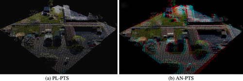
A utility is developed which takes the following inputs: (1) the point dataset, (2) the texture corresponding to the point dataset, and (3) the mode of visualization (mono or anaglyph). Each of the points in the dataset is mapped to the visualization engine. Using the texture mapping function, the color attribute for each of the points is calculated, and the list sent to the visualization engine. This mode of visualization is named as PTS. The mono-mode of visualization is named PL-PTS and the corresponding anaglyph mode is named AN-PTS.

2.2.3. 2-simplex-based visualization

2-simplices or triangles can be generated in two ways: (1) use the planimetric coordinates of each of the points to compute a Delaunay triangulation or (2) use the 3D coordinates of the points to compute a Delaunay tetrahedralization and then explode each of the tetrahedrons in the list to the corresponding facets.

Delaunay triangulation and tetrahedralization are computed using the QuickHull (QHULL) (Barber, Dobkin, and Huhdanpaa 1996) utility (http://www.qhull.org/). The 2-simplices required for the purposes of visualization are produced in the manner described in the following paragraphs:

2.2.3.1. Delaunay triangulation (DTRI)

The planimetric coordinates of the points given in a dataset are passed on to the QHULL utility to generate the triangulation. The texture coordinates are obtained from the texture mapping function. The points, texture coordinates, texture, and the display mode (nonstereo or anaglyph) are passed to the OpenSceneGraph display using a command line utility. The nonstereo mode of display is termed PL-DTRI and the stereo mode of display is termed AN-DTRI.

2.2.3.2. Delaunay triangulation followed by trimming (TDTRI)

The triangulation Δ is first computed. For each of the triangles Δ∈Δ, the maximum edge length is calculated. All triangles having are retained, and the rest are deleted. Here is a trimming threshold provided by the user, indicating the largest triangle that should be retained. A command line utility which takes the following inputs, was designed: (1) the list of the points, (2) the trimming threshold, (3) the texture, and (4) the mode of visualization (nonstereo or anaglyph). The nonstereo mode of display is termed PL-TDTRI and the stereo mode is termed as AN-TDTRI.

2.2.3.3. Delaunay tetrahedralization followed by exploding and trimming (TDTET)

The tetrahedralization is generated using the QHULL utility for a given list of points. Each of the tetrahedra generated from the process is exploded into corresponding facets, thus generating the list of triangles Δ^T. All triangles having are retained, and the rest are deleted, where is a trimming threshold provided by the user. A command line utility was designed which takes the following inputs: (1) the list of the points, (2) the trimming threshold , (3) the texture, and (4) the mode of visualization (nonstereo or anaglyph). The nonstereo mode of display is term PL-TDTET and the stereo mode is termed as AN-TDTET.

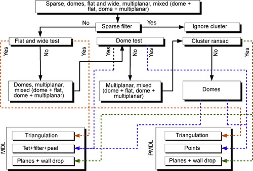
2.2.4. Heuristic-based reconstruction and visualization

Delaunay triangulation uses only the planimetric coordinates of the data provided to the algorithm. Therefore, objects like trees that contain multistoreyed information, will not be rendered well by the Delaunay triangulation. One might consider using the Delaunay tetrahedralization for representing such objects. Thus, the need for developing the heuristics for reconstruction arises where the algorithm would decide whether to apply triangulation or tetrahedralization for an object. This is done using two steps (1) data partitioning and (2) cluster generalization.

2.2.4.1. Data partitioning

To apply triangulation and tetrahedralization separately, point data should separate or partition the data into different sets. An elementary point data visualization of LiDAR datasets tells us that terrain objects are represented as arbitrarily shaped and spatially collocated points. Ester et al. (1996) suggests that Density Based Spatial Clustering of Applications with Noise (DBSCAN) algorithm is able to extract arbitrarily shaped clusters of points. Therefore, partitioning is achieved using DBSCAN.

Generally, distances are computed using the Euclidean distance metric. However, LiDAR datasets can contain multiple points having the same coordinates. Therefore, the following modified Euclidean metric is used for DBSCAN in order to avoid cases where the value of the distance is zero:

(1)

DBSCAN requires two different inputs: (1) a distance threshold ε, and (2) a threshold minPts. DBSCAN treats a point as a member of a cluster if a sphere of radius ε contains more than minPts points.

2.2.4.2. Cluster generalization

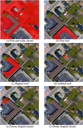
Following the spatial clustering of the data points using DBSCAN, various types of clusters are formed. These clusters are divided into the following classes (1) sparse; (2) flat and wide; (3) dome-shaped clusters; and (4) clusters potentially containing planes. Heuristics are then developed to generalize each of these clusters based on its type. The measures for these classes and the heuristics are presented in Ghosh and Lohani (2011).

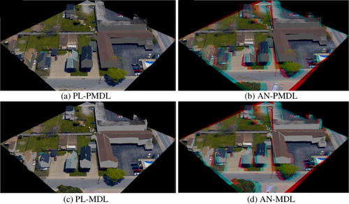
This study uses two different variants of the cluster generalization method studied by Ghosh and Lohani (2011) that are described here. The first variant is termed PMDL where the dome-shaped clusters are passed to the visualization engine as a point cloud. The second variant is termed MDL, where the dome-shaped clusters are processed as described by Ghosh and Lohani (2011). The nonstereo modes of visualization are named as PL-PMDL and PL-MDL, respectively, and the anaglyph modes of visualization are named as AN-PMDL and AN-MDL, respectively. These processing pipelines are illustrated in Figure 1.

Figure 1. Heuristic-based processing pipelines: MDL and PMDL.

2.2.5. Processing and reconstruction through professional software

The classification of LiDAR data points has been studied in detail in the literature, especially in the sector of identifying the terrain and the detection and reconstruction of buildings.

The TerraSolid package is used to classify the LiDAR datasets. The buildings were reconstructed using the computer-aided design (CAD) digitization capabilities of TerraSolid and Bentley Microstation. Trees present in the scenes were replaced by Real Photorealistic Content (RPC) models. Finally, walk-through videos were generated through Bentley Microstation using the CAD reconstruction and the texture corresponding to the given datasets. This video-based pipeline is termed as PL-CAD.

2.3. Comparing the visualization pipelines

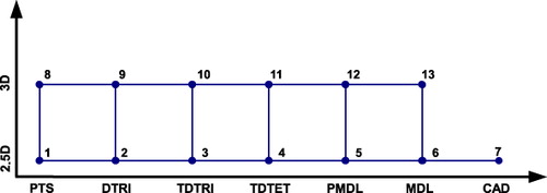
There are 13 different visualization pipelines as listed in Table 3. In this study, the different visualization pipelines are compared qualitatively in terms of depth and feature perception. This was done by conducting a survey, where the participants were presented with a questionnaire and the outputs rendered by the various pipelines. This subsection describes the design of the questionnaire, the methodology of feedback collection from the participants, and the statistical methodology to compare the various pipelines.

Table 3. Different visualization pipelines studied in this paper.

Pipeline	Nonstereo mode	Stereo mode
Point-based visualization	PL-PTS	AN-PTS
Delaunay triangulation	PL-DTRI	AN-DTRI
Delaunay triangulation followed by trimming	PL-TDTRI	AN-TDTRI
Delaunay tetrahedralization followed by exploding tetrahedra and trimming	PL-TDTET	AN-TDTET
Heuristic-based processing. Dome-shaped clusters rendered as points	PL-PMDL	AN-PMDL
Heuristic-based processing. Dome-shaped clusters generalized	PL-MDL	AN-MDL
CAD-based processing and video generation	PL-CAD

2.3.1. Design of the questionnaire

A questionnaire is first designed to collect feedback from the participants with the following questions:

1. How well do you rate the depth perception in the scene?

2. How would you rate the overall display quality of the scene?

3. How would you rate the quality of the buildings?

4. How would you rate the quality of the trees?

5. How would you rate the quality of the roads?

6. How would you rate the quality of the vehicles?

Dawes (2008) proved that ratings based on a scale of 5 or 7 tended to shift the mean to the higher side and that a 10-point rating scale was comparatively better. Therefore, for each participant, scores are collected on a 10-point scale as responses to each of the above questions for each of the outputs from the visualization pipelines (see Table 3). A score of 1 means the ‘worst’ and a score of 10 means the ‘best.’

An interface was designed which alternately displays the outputs of the visualization pipelines and the questionnaire to the participants. The interface was capable of presenting the different renderings from the various pipelines in a given order.

Since, there are 13 different visualization pipelines and 5 datasets, there are 5 × (13!) different ways of presenting the outputs to the participants.¹ Confounding is used to limit the number of ways to present the outputs of the various pipelines. The visualization pipelines are, therefore, laid down as nodes shown in Figure 2. A ‘graph’ is then created where these nodes are joined by lines with a jump of one unit either in the x-direction or in the y-direction. Hamiltonian paths are calculated using Mathematica to determine the order of presentation of the 13 pipelines to the participant. These different paths also avoid the existence of bias in the data obtained from the experiment (Vajta et al. 2007).

Figure 2. Layout of various visualization pipelines for confounding and determination of Hamiltonian paths.

2.3.2. Statistical tests for comparison

The 13 visualization pipelines are compared using the data obtained from the experiment. Let us suppose that n participants agree to participate. The number of visualization pipelines is k = 13. Let us suppose that the ith participant gives a score of s _ij to the output of the jth pipeline.

The null hypothesis is framed as H ₀ : ‘All processes are similar.’ The alternative hypothesis would be to prove otherwise. Table 4 brings out the various calculations and statistical measures for Friedman's test (Friedman 1937, 1939) and Kruskal–Wallis test (Kruskal and Wallis 1952) as brought out by Gibbons and Chakraborti (2010).

Table 4. Notation, statistic and post-hoc analyzes for Friedman's test and Kruskal–Wallis test.

Friedman's test	Kruskal–Wallis test
Notations
: rank of sij, in	: rank of sij, in
Statistic
Friedman's: t denotes the number of row-wise ties for each row-wise rank
Kruskal–Wallis: t denotes the number of overall ties for each rank
Null hypothesis rejected, if for a level of significance α:
Post-hoc analysis: Processes i and j are termed different if:

In case the null hypothesis is rejected for a given level of significance α, i.e. the k processes are not similar, then the respective post-hoc analyzes have to be conducted. Since and , j = 1,…, k are real numbers, j ₁, j ₂,…, j _k and can be found such that and . Thus all the processes can be attributed hypothetical ranking sets from 1 to k, each for Friedman's and Kruskal–Wallis tests. If two processes are found similar, the same hypothetical rank is attributed as per the standard competition ranking scheme.

The hypothetical ranking sets are confirmed using Page's trend test. If Y _j denotes the hypothetical ranking of the jth column, obtained through some process, then the L-statistic is given by:

The value defined by Page (1963) is given as follows:

approximately follows the central distribution with a degree of freedom as 1. Gibbons and Chakraborti (2010) have applied a continuity correction to the above formula, thus defining Z² as follows:

Z² is distributed according to the central distribution with a degree of freedom 1. Therefore, if , where α is the level of significance, then the null hypothesis is rejected and the hypothetical ranking of the processes is accepted.

3. Results and discussion

3.1. Point-based visualization

Since the data captured is from an airborne platform, the scanner captures the top of the terrain features. Thus, although the data is perceivable from all the directions, it was also seen from several tests carried out with the participants that they tend to zoom out of the scene to perceive the features. In this mode of visualization, features at the background intervene with the features located in the foreground, thus leading to confusion in the recognition of the features present in the dataset.

The outputs of the point-based visualization pipelines are shown in Figure 3.

Figure 3. Outputs from the point-based visualization themes.

3.2. 2-simplex-based visualization

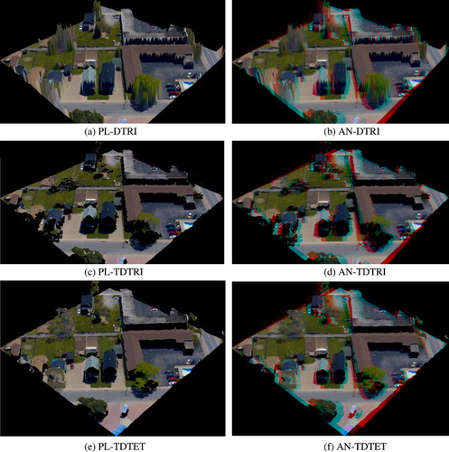
Trees captured through the altimetric LiDAR instrument contain multiple storeys of the vegetation canopy. Therefore, the triangulation algorithm does not render the trees well. Further, in a Delaunay triangulation, the walls of the buildings are interpolated as sloping surfaces instead of being vertical. In a trimmed Delaunay triangulation-based pipeline, the scenes contained objects floating in the air with apparent holes in the place of trees.

Tetrahedralization leads to smoother building roofs. However, since the process involved exploding the tetrahedrons, there were more triangles compared to the triangulation-based environment. The restitution was therefore slow. The trees were however well represented. The outputs from these pipelines are shown in Figure 4.

Figure 4. Outputs of 2-simplex-based pipelines.

3.3. Heuristic-based visualization pipelines

Visual experience through 2-simplices revealed that while buildings were better restituted through triangulation, trees were rendered better using tetrahedra. This gave rise to the need for the development of heuristics and a heuristic-based visualization pipeline (Ghosh and Lohani 2011).

3.3.1. Efficacy of DBSCAN for identifying clusters

DBSCAN uses minPts and ε as thresholds. From a preliminary visualization of the points, it was observed that a group of 3 or less points lying apart from the remaining point cloud could be labeled as outliers. Thus a value of minPts = 3 was chosen. An experiment was conducted to determine a proper value of ε.

The LiDAR datasets were first visually clustered using TerraScan and kept separately. DBSCAN was then executed for a fixed value of minPts = 3 and varying values of ε from a very low 0.3 m to a high 4.0 m in small steps of 0.01 m to generate various clustering outputs. The Adjusted Rand Index (ARI) (Hubert and Arabie 1985) was used to compare the results of the DBSCAN clustering with the visual clustering. It was found that the ARI was highest when ε = 1.0.

DBSCAN was re-executed for the best clustering threshold combination (minPts = 3, ε = 1.0), and then each of the clusters was overlayed on the georectified aerial image of the corresponding dataset using the MATLAB Mapping Toolbox. It can be seen from Figure 5 that DBSCAN has been able to successfully extract the clusters of arbitrary shapes, which are actually the objects on the terrain.

Figure 5. Outputs of the clustering algorithm (DBSCAN). The screen-shots have been provided for one of the datasets.

DBSCAN took approximately 550 seconds to cluster each of the datasets. The computational time for DBSCAN may be reduced by using the k–d tree spatial indexing method (Bentley 1975).

3.3.2. Efficacy of the heuristics

The generated clusters were passed through the heuristics. An experiment was conducted where different clusters were picked up from different clustering outputs of the chosen datasets. It was seen that the heuristics were able to identify the types of the clusters with a good accuracy (see Table 5). The selected parameters for the heuristics are described in Ghosh and Lohani (2011).

Table 5. Contingency table describing the efficacy of the heuristics.

		Manually identified
Heuristics		Sparse	Flat and wide	Dome shaped	Potentially containing planes
Sparse		5	0	0	0
Flat and wide		0	5	0	0
Dome shaped		0	0	15	1
Potentially containing planes		0	0	1	13

Source: Ghosh and Lohani (2011).

3.3.3. Visualization through the heuristic-based pipelines

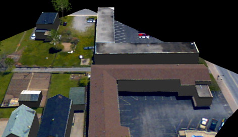
The visualization through the heuristic-based pipelines are shown in Figure 6 through screenshots. It is seen through visual comparison that buildings and trees are rendered comparatively better in PL-MDL and AN-MDL modes. Also the buildings present in the scene are rendered with vertical walls.

Figure 6. Visualization through the heuristic-based pipelines.

3.4. Visualization through PL-CAD

While the TerraSolid package was efficient in extracting the ground and detecting and reconstructing the buildings, it required Real Photorealistic Content models for the reconstruction of the trees. For the purposes of rendering, the capabilities of Bentley Microstation were used to generate the walk-through videos after complete classification and reconstruction. The vehicles in the scenes were seen to be flattened to the ground since there is no existing algorithm in the TerraSolid package for detecting vehicles. The visualization through the classification and CAD-based pipeline is presented in Figure 7.

Figure 7. CAD-based visualization.

3.5. Conduction of the experiment

The comparison of the different pipelines was done through a survey-based experiment. Sixty undergraduate students of the third year at the Department of Civil Engineering, IIT, Kanpur, agreed to participate. None of the participants were exposed to LiDAR datasets and neither were they exposed to the domain of visualization in their curriculum. Participants were allotted 45-minute appointment schedules for providing feedbacks to the various pipelines in terms of scores. During the course of the experiment, lighting and cooling were maintained constant. Noises and other disturbances were kept to the bare possible minimum.

At the beginning of each of the experiments, a participant was explained about the scoring methodology to be followed. The participant was asked to attribute scores to each output independent of the other. The participant was then presented with a few anaglyph photographs in an increasing order of complexity and was asked either to count the number of objects or rank the objects in the order of distance from the viewer. This was done in order to test and acquaint the participant in depth perception. After this training, the graphical user interface (GUI) designed for the purpose of collecting scores was presented to the participant. The GUI presented the outputs for the 13 pipelines in an order determined by the Hamiltonian path for a single dataset. For each of the participants, a different dataset was selected. The scores obtained from a participant were stored in a data file in binary format in the hard disk.

3.6. Data organization and analysis

There are six questions in the questionnaire and the number of participants is 60. LibreOffice Calc spreadsheet software is used to read the data and tabulated in six different worksheets (one worksheet for each question). Friedman's test (Friedman 1937, 1939) and Kruskal–Wallis test (Kruskal and Wallis 1952) were conducted on each of the sheets. The ranks obtained from each of the sheets were tabulated again to compute the overall rankings.

3.6.1. Initial analysis

Pearson's goodness-of-fit test and histograms verified that the distributions for the scores received for each of the visualization pipelines were not normally distributed. Thus parametric methods like analysis of variance (ANOVA) or multivariate analysis of variance (MANOVA) are unfit for testing the null hypothesis. Thus nonparametric Friedman's test and Kruskal–Wallis test, and their corresponding post-hoc analyzes are, therefore, suited to examine which methods have performed the best in terms of feature and depth perception. For all purposes, the level of significance α as 0.05 is used.

3.6.2. Results from Friedman's test

The Friedman test (Friedman 1937, 1939) is first used to test the null hypothesis. The results of Friedman's test for each of the questions are presented in Table 6. With the level of significance α = 0.05, it is seen that the null hypothesis cannot be accepted for all of the questions.

Table 6. Q and H statistic and P values for all the questions.

	Friedman's test		Kruskal–Wallis test
Q. No.	Q statistic	P value	H statistic	P value
1	3022.5772	≈0.00E+000	141.9547	2.4132E–024
2	2662.1177	≈0.00E+000	133.8197	1.0541E–022
3	2543.9386	≈0.00E+000	131.3701	3.2757E–022
4	2338.7483	≈0.00E+000	126.9111	2.5692E–021
5	2444.8502	≈0.00E+000	106.1568	3.4340E–017
6	1610.1333	≈0.00E+000	71.4586	1.7070E–010

3.6.3. Results from Kruskal–Wallis test

The test of the null hypothesis is also done with Kruskal–Wallis test (Kruskal and Wallis 1952). The results of Kruskal–Wallis test for each of the questions are given in Table 6. With the level of significance α = 0.05, it is seen that the null hypothesis cannot be accepted for all of the questions.

3.6.4. Question-wise rankings from post-hoc analysis

The post-hoc analysis of Friedman's test and Kruskal–Wallis test are used to determine the performance differences in terms of depth and feature perception for the different visualization pipelines (Gibbons and Chakraborti 2010). The hypothetical rankings determined through the post-hoc analysis are confirmed using Page's trend test (Page 1963). The hypothetical rankings obtained through the post-hoc analyzes and their confirmations using Page's trend test are presented in Table 7. It is seen that the rankings for both the tests and for all the questions are consistent as shown by Spearman's ρ, Kendall's , and Goodman and Kruskal's rank correlation coefficients (Kendall 1938; Goodman and Kruskal 1954; Spearman 1987). For all the questions, it is seen that the P values for Page's trend test, are lesser for the rankings obtained from the post-hoc analysis of Friedman's test than that of the post-hoc analysis of Kruskal–Wallis test. Therefore, it can be said that the rankings for Friedman's test are more acceptable at a significance level of α = 0.05.

Table 7. Question-wise ranks for Friedman's test (FT) and Kruskal–Wallis test (KW), their confirmation using Page's trend test and their consistencies using Spearman's ρ, Kendall's τ and Goodman and Kruskal's γ.

	Question 1		Question 2		Question 3		Question 4		Question 5		Question 6
	FT	KW	FT	KW	FT	KW	FT	KW	FT	KW	FT	KW
PL-PTS	13	13	13	13	13	13	12	12	13	13	13	13
PL-DTRI	8	7	8	8	9	8	10	9	8	8	7	7
PL-TDTRI	12	12	11	11	12	12	13	13	10.5	11	11	11
PL-DTET	10.5	10	10	10	11	10	9	8	10.5	10	10	9
PL-PMDL	10.5	11	7	7	6	6	11	11	9	7	8	8
PL-MDL	9	9	9	9	7	7	8	10	7	9	9	10
PL-CAD	2.5	2	1	1	1	1	1	1	3	1	6	6
AN-PTS	7	8	12	12	10	11	6	7	12	12	12	12
AN-DTRI	4	3	5	4	4	4	4	4	2	3	3	3
AN-TDTRI	6	6	6	6	8	9	5	6	6	6	5	5
AN-DTET	2.5	4	2	3	5	5	2	2	5	5	2	2
AN-PMDL	5	5	4	5	2	3	7	5	4	4	4	4
AN-MDL	1	1	3	2	3	2	3	3	1	2	1	1
	8.49E3	2.15E2	8.48E3	1.94E2	8.51E3	1.87E2	8.49E3	1.53E2	8.49E3	1.67E2	8.51E3	1.19E2
P value	0.00E+00	1.2E−48	0.00E+00	4.3E−44	0.00E+00	1.2E−42	0.00E+00	3.4E−35	0.00E+00	3.7E−38	0.00E+00	8.5E−28
ρ	0.9835		0.9890		0.9835		0.9670		0.9601		0.9945
τ	0.8974		0.9487		0.9231		0.8974		0.8461		0.9743
γ	0.8974		0.9487		0.9231		0.8974		0.8461		0.9743

3.6.5. Overall rankings

To obtain the overall rankings using the Friedman's test, for the various processes listed in Table 3, the question-wise rankings are used. The same null hypothesis test and the post-hoc analysis are conducted again on the question-wise rankings. It is found that the Q-statistic for this test is 819.6610 and the P value is 1.0047E–167. However, in this case, it is seen that Friedman's test is not able to give a very good ranking, inspite of the processes being different, due to the fact that the right-hand side of inequality for post hoc analysis is a large number, thus giving rise to too many ties. Therefore, Kruskal–Wallis test is used to obtain the overall rankings for the processes.

For a layman user, a good visualization pipeline is one which represents the various features on the terrain as they appear in real world. The features being perceived by the participants were buildings, trees, roads, and vehicles. Before analyzing the scores of the experiment, it was expected that the PL-CAD would perform the best in terms of depth and feature perception, since the features like buildings were manually reconstructed and the trees present on the terrain were replaced by Real Photorealistic Content cells. These tasks were performed using TerraScan, a module of the TerraSolid software.

It can be seen from Table 7 that anaglyph-based visualization pipelines have generally received better rankings. Almost every participant expressed appreciation for the realistic representation of the data in the anaglyph mode of visualization. Since laymen are not used to see the features of the terrain in the point format, low ratings have been received by the point-based visualization pipelines, namely, PL-PTS and AN-PTS. Table 7 also reveals the same. It was also observed during the experiment that the participants usually zoomed out while visualizing the point-based pipelines.

The triangulation-based pipelines, namely, PL-DTRI and AN-DTRI, give rise to pseudo walls of the buildings which are not vertical. However, the building roofs are rendered properly. PL-TDTRI and AN-TDTRI have the building roof hanging in the space and, therefore, have poor ratings. Further, PL-TDTET and AN-TDTET have smoother building roofs compared to the triangulation-based pipelines, but they are still hanging in the space. The buildings in the terrain are reconstructed manually using the process of classification for PL-CAD. Thus, buildings are represented the best in the PL-CAD pipeline and also receive the best scores and ranks from the participants, closely followed by AN-MDL and AN-PMDL.

The trees present in the terrain reflect the laser beams not only from the periphery of their respective canopies but also from within it. The Delaunay triangulation only considers one of the points which have the same values of x and y coordinates and different z coordinates. As a result, there is a loss of 3D information when a triangulation is generated from the raw datasets. Therefore, PL-DTRI and AN-DTRI do not render the trees properly. Also, the culling of the long triangles in PL-TDTRI and in AN-TDTRI leads to the disappearance of the trees on the terrain. Consequently, these visualization pipelines receive lower ranks for the perception of trees. On the other hand, the visualization pipelines PL-TDTET and AN-TDTET were designed to address the problem faced by the triangulation algorithm in rendering trees. However, the canopies of the trees are found suspended in space. On the contrary, the trees are replaced by RPC models in PL-CAD. Effectively, the best ranks for trees are obtained by PL-CAD followed by AN-TDTET.

The 2-simplex-based and the heuristic-based themes are able to render the vehicles satisfactorily. On the other hand, the TerraScan module used for the process of classification did not have any specific routine for extracting vehicles. Therefore, the vehicles do not appear in 3D in PL-CAD. Eventually, PL-CAD received lower rankings for vehicles. It is to be noted here that although no separate treatment was given for vehicles in the development of the heuristics, vehicles are rendered satisfactorily as they are grouped as a part of the terrain during the clustering process. The roads were visible clearly in most of the visualization pipelines, and high scores were received from the participants for all of them.

Through Friedman's test and subsequent post-hoc analysis, it is seen that the overall rankings are best in terms of feature and depth perception for AN-MDL, followed by PL-CAD and AN-TDTET on second and third ranks. On the other hand, through Kruskal–Wallis test and subsequent post-hoc analysis, it is seen that the overall rankings are best for PL-CAD, followed by AN-MDL and AN-TDTET on second and third ranks. These rankings have also been verified statistically using Page's trend test. The ranks assigned by Friedman's test and Kruskal–Wallis test are also found to be consistent using the rank correlation tests given in Kendall (1938), Goodman and Kruskal (1954), and Spearman (1987). However, it is seen from Table 8 that with the rankings calculated through Friedman's test and post-hoc process, the P values are smaller compared to those obtained from Kruskal–Wallis test and post-hoc analysis. Therefore, the statistic obtained from Friedman's test and post-hoc analysis rejects the null hypothesis more strongly compared to the statistic obtained from Kruskal–Wallis test and post-hoc analysis. The rankings obtained from Friedman's test and post-hoc analysis are, therefore, more acceptable.

Table 8. Overall rankings by using average column ranks for all questions and all the visualization pipelines.

Q. No.	PL-PTS	PL-DTRI	PL-TDTRI	PL-DTET	PL-PMDL	PL-MDL	PL-CAD	AN-PTS	AN-DTRI	AN-TDTRI	AN-DTET	AN-PMDL	AN-MDL
1	76	56	67	63	64	59	5	57	10	31	13	16	4
2	77	44	66	60	38	50	3	68	17	34	15	19	8
3	75	45	71	62	35	37	2	65	23	46	29	7	6
4	69	52	70	51	61	55	1	42	30	41	14	39	25
5	78	43	53	49	40	47	9	73	18	27	26	20	12
6	74	33	58	48	36	54	32	72	22	28	21	24	11
Sum	449	273	385	333	274	302	52	377	120	207	118	125	66
Avg.	74.83	45.50	64.17	55.50	45.67	50.33	8.67	62.83	20.00	34.50	19.67	20.83	11
H	253.4417
P value	2.6195E–047 (null hypothesis not accepted)
Rank	13	7.5	10.5	10.5	7.5	10.5	1.5	10.5	4	6	4	4	1.5
	59.4170
	1.2756E–014

Note: Rankings are confirmed through Page's trend test.

The overall rankings are calculated using Kruskal–Wallis test and its corresponding post-hoc analysis, as the post-hoc analysis of Friedman's test does not give comprehensive information for overall ranking. The question-wise column averages for earlier Kruskal–Wallis test are used as an input for the overall ranking. The results are presented in Table 8. From the rankings obtained, it can be said that the heuristic-based pipeline AN-MDL (Ghosh and Lohani 2011) performs almost similar to the PL-CAD pipeline where manual classification and reconstruction are involved, in terms of feature and depth perception.

3.7. Efficiency of the novel pipelines and their applicability to datasets of larger sizes

The efficiency of a visualization pipeline for LiDAR datasets depends on how effectively the various features on the terrain are rendered by the visualization engine. The novel pipelines, namely, MDL and PMDL, are based on spatial clustering and subsequent reconstruction using heuristics. The pipelines were developed in order to allow a ‘quick’ visualization of the LiDAR data. While the novel pipelines took an average of 600 seconds of computational time for processing and rendering, the classification-based method took an average of about 3 hours (10,800 seconds) for complete CAD reconstruction, for the datasets used in this paper.

Spatial data structures like k–d trees can reduce the time for nearest neighbor search, thus saving computational time for generating the spatial clusters. Thus, larger point clouds may be first divided into smaller tiles, and then each of these tiles could be subjected to spatial clustering followed by heuristic-based reconstruction. This technique would be effective even for those computers which are not capable of parallel processing of data.

4. Conclusions and future directions

LiDAR dataset sizes are very large even for very small areas. The research challenge posed by MacEachren and Kraak (2001) for visualizing large geospatial datasets has provoked the interest in the direction of research proposed in this paper. Mapping using LiDAR datasets requires feature extraction, generalization, and then visualization. This paper has discussed some conventional pipelines of visualizing LiDAR datasets, namely, point-based and triangulation-based and some more pipelines which have been developed, namely, tetrahedralization-based and heuristic-based. These visualization pipelines were statistically compared through the design of an experiment and statistical tests.

The analysis of the data obtained through the experiment used in this study has revealed equivalent performances from PL-CAD model and the AN-MDL visualization scheme, in terms of depth and feature perception. The 2-simplex-based pipelines, namely, PL-DTET and AN-DTET rendered building roofs properly, but the renderings of the trees were not close to reality. On the other hand, it was observed during the experiments that although PL-TDTET and AN-TDTET were successful in rendering trees, the restitution was slow owing to the large number of triangles generated during the process. The point-based visualization pipelines performed badly in terms of feature recognition as there was significant confusion among the foreground and background features. These observations are also supported by the scores obtained from the participants and the statistical rankings obtained thereafter.

It is understood that this is the first step in the direction of statistical comparison of visualization pipelines for LiDAR datasets. Some of the future improvements in the study are highlighted in the following paragraphs.

1. Size of the dataset: The LiDAR datasets used in this study were of small area viz. 100 × 100 m. However, all the pipelines studied in this paper can be extended to larger datasets by dividing each dataset into manageable tiles. A preparation for developing an experiment involving larger datasets is being planned.

2. Design of the experiment for geovisualization and choice of participants: An experiment design on the lines of Tobón (2005) using a task-based methodology and levels of participants varying from novice to expert is planned for the future.

3. Parameters for the visualization pipelines: All visualization pipelines in this study use the georectified aerial photograph as a coloring or draping element. Future studies could also investigate the possibility of including pipelines where height-based coloring or all points with the same color, or absence or presence of shadows are used as additional parameters for the experiment.

4. Statistical methodology for hypothesis testing: The statistical methodology applied here uses a univariate and recursive approach. In the future, a multivariate method is planned to be developed and used for the ranking of the different pipelines.

Acknowledgments

The first author would like to thank Indian Institute of Technology, Kanpur, where a major portion of this work was carried out. In addition, the authors would like to thank Optech Inc. for sharing the data and Geokno for creating the orthophotos for this study. The authors would also like to thank the two anonymous reviewers for adding quality to the previous versions of this paper.

Notes

1. The YouTube links for the various outputs from the five datasets listed earlier have been given in the page, http://home.iitk.ac.in/∼blohani/Datadetails.html.

References

- Awrangjeb, M., C. Zhang, and C. Fraser. 2011. “Automatic Reconstruction of Building Roofs Using Lidar and Multispectral Imagery.” In Digital Image Computing Techniques and Applications (DICTA), 2011 International Conference, pp. 370–375. Noosa: IEEE.
- Axelsson, P. 2001. “Ground Estimation of Laser Data Using Adaptive TIN Models.” In Proceedings of OEEPE Workshop on Airborne Laserscanning and Interferometric SAR for Detailed Digital Elevation Models, Publication No. 40, CDROM. Stockholm: Royal Institute of Technology.
- Barber, C. B., D. P. Dobkin, and H. Huhdanpaa. 1996. “The Quickhull Algorithm for Convex Hulls.” ACM Transactions on Mathematical Software 22 (4): 469–483. 10.1145/235815.235821.
- Bentley, J. L. 1975. “Multidimensional Binary Search Trees Used for Associative Searching.” Communications of the ACM 18: 509–517. 10.1145/361002.361007.
- Błaszczak-Ba̧k, Ã. Ň., A. Janowski, W. Kamiński, and J. Rapiński. 2011. “Optimization Algorithm and Filtration Using the Adaptive TIN Model at the Stage of Initial Processing of the ALS Point Cloud.” Canadian Journal of Remote Sensing 37 (6): 583–589. 10.5589/m12-001.
- Brandtberg, T. 2002. “Individual Tree-based Species Classification in High Spatial Resolution Aerial Images of Forests Using Fuzzy Sets.” Fuzzy Sets and Systems 132 (3): 371–387. 10.1016/S0165-0114(02)00049-0.
- Brandtberg, T., T. Warner, R. Landenberger, and J. McGraw. 2003. “Detection and Analysis of Individual Tree Crowns in Small Footprint, High Sampling Density LiDAR Data from the Eastern Deciduous Forest in North America.” Remote Sensing of Environment 85: 290–303. 10.1016/S0034-4257(03)00008-7.
- Brovelli, M. A., M. Cannata, and U. Longoni. 2002. “Managing and Processing LIDAR Data within GRASS.” In Proceedings of GRASS Users Conference, 29. Trento: University of Trento, Italy, September 11–13.
- Brovelli, M. A., M. Cannata, and U. M. Longoni. 2004. “LIDAR Data Filtering and DTM Interpolation within GRASS.” Transactions in GIS 8 (2): 155–174. 10.1111/j.1467-9671.2004.00173.x.
- Caldwell, J., and S. Agarwal. 2013. “LiDAR Best Practices.” Earth Imaging Journal. Accessed January 5, 2014. http://eijournal.com/2013/lidar-best-practices.
- Clode, S., F. Rottensteiner, and P. J. Kootsookos. 2005. “Improving City Model Determination by Using Road Detection from LiDAR Data.” In Joint Workshop of ISPRS and the German Association for Pattern Recognition (DAGM). Vienna: Object Extraction for 3D City Models, Road Databases and Traffic Monitoring - Concepts, Algorithms, and Evaluation’ (CMRT05).
- Dawes, J. 2008. “Do Data Characteristics Change According to the Number of Scale Points Used? An Experiment Using 5-point, 7-point and 10-point Scales.” International Journal of Market Research 50 (1): 61–77.
- Ester, M., H.-P. Kriegel, J. Sander, and X. Xu. 1996. “A Density-based Algorithm for Discovering Clusters in Large Spatial Databases with Noise.” In Proceedings of the Second International Conference on Knowledge Discovery and Data Mining (KDD-96), edited by E. Simoudis, J. Han, and U. M. Fayyad, 226–231. Portland, OR: AAAI Press.
- Forlani, G., C. Nardinocchi, M. Scaioni, and P. Zingaretti. 2003. “Building Reconstruction and Visualization from LiDAR Data.” In The International Archives of the Photogrammetry, Remote Sensing and Spatial Information Sciences, volume XXXIV, Part 5/W12. Ancona: ISPRS.
- Friedman, M. 1937. “The Use of Ranks to Avoid the Assumption of Normality Implicit in the Analysis of Variance.” Journal of the American Statistical Association 32 (200): 675–701. 10.1080/01621459.1937.10503522.
- Friedman, M. 1939. “A Correction: The Use of Ranks to Avoid the Assumption of Normality Implicit in the Analysis of Variance.” Journal of the American Statistical Association 34 (205): 109.
- Fujisaki, I., D. L. Evans, R. J. Moorhead, D. W. Irby, M. J. M. Aragh, and S. D. Roberts. 2003. “Lidar Based Forest Visualization: Modeling Forest Stands and User Studies.” In ASPRS Annual Conference. Fairbanks, AK: ASPRS.
- Ghosh, S., and B. Lohani. 2011. “Heuristical Feature Extraction from LiDAR Data and Their Visualization.” In Proceedings of the ISPRS Workshop on Laser Scanning 2011, edited by D. D. Lichti and A. F. Habib. International Society of Photogrammetry and Remote Sensing, University of Calgary, Canada, volume XXXVIII. http://www.isprs.org/proceedings/XXXVIII/5-W12/Papers/ls2011_submission_38.pdf.
- Gibbons, J. D., and S. Chakraborti. 2010. Nonparametric Statistical Inference. 5th ed. Boca Raton: Chapman and Hall.
- Goodman, L. A., and W. H. Kruskal. 1954. “Measures of Association for Cross Classifications.” Journal of the American Statistical Association 49 (268): 732–764.
- Harvey, W. A., and D. M. McKeown, Jr. 2008. Automatic Compilation of 3D Road Features Using LIDAR and Multi-spectral Source Data. Portland, OR: ASPRS. Accessed January 1, 2014. http://www.terrasim.com/brochures/events/2008/2008ASPRS_Paper.pdf.
- Hermosilla, T., L. A. Ruiz, J. A. Recio, and J. Estornell. 2011. “Evaluation of Automatic Building Detection Approaches Combining High Resolution Images and LiDAR Data.” Remote Sensing 3 (6): 1188–1210. 10.3390/rs3061188.
- Hu, X., C. V. Tao, and Y. Hu. 2004. “Automatic Road Extraction from Dense Urban Area by Integrated Processing of High Resolution Imagery and Lidar Data.” In IAPRSSIS. Vol. XXXV, edited by O. Altan, 288–292. Istanbul: ISPRS. Accessed January 1, 2014. http://www.cis.rit.edu/~cnspci/references/dip/urban_extraction/hu2004.pdf.
- Hubert, L., and P. Arabie. 1985. “Comparing Partitions.” Journal of Classification 2: 193–218. 10.1007/BF01908075.
- Hyyppä, J., H. Hyyppä, D. Leckie, F. A. Gougeon, X. Yu, and M. Maltamo. 2008. “Review of Methods of Small-footprint Airborne Laser Scanning for Extracting Forest Inventory Data in Boreal Forests.” International Journal of Remote Sensing 29 (5): 63–78.
- Kendall, M. 1938. “A New Measure of Rank Correlation.” Biometrika 30 (1–2): 81–89.
- Kobler, A., N. Pfeifer, P. Ogrinc, L. Todorovski, K. Ostir, and S. Dzeroski. 2007. “Repetitive Interpolation: A Robust Algorithm for DTM Generation from Aerial Laser Scanner Data in Forested Terrain.” Remote Sensing of Environment 108: 9–23. http://www.sciencedirect.com/science/article/pii/S003442570600424X. 10.1016/j.rse.2006.10.013.
- Kraus, K., and N. Pfeifer. 1998. “Determination of Terrain Models in Wooded Areas with Airborne Laser Scanner Data.” ISPRS Journal of Photogrammetry and Remote Sensing 53: 193–203. 10.1016/S0924-2716(98)00009-4.
- Kreylos, O., G. Bawden, and L. Kellogg. 2008. “Immersive Visualization and Analysis of Lidar Data.” In Advances in Visual Computing, edited by G. Bebis, R. Boyle, B. Parvin, D. Koracin, P. Remagnino, F. Porikli, J. Peters, J. Klosowski, L. Arns, Y. Chun, T.-M. Rhyne, and L. Monroe, 846–855. Berlin: Springer, Lecture Notes in Computer Science, volume 5358, ISBN 978-3-540-89638-8. http://dx.doi.org/10.1007/978-3-540-89639-5_81.
- Kruskal, W. H., and W. A. Wallis. 1952. “Use of Ranks in One-criterion Variance Analysis.” Journal of the American Statistical Association 47 (260): 583–621. 10.1080/01621459.1952.10483441.
- Lemmens, M. J. P. M., H. Deijkers, and P. A. M. Looman. 1997. “Building Detection by Fusing Airborne Laser-altimeter DEMs and 2D Digital Maps.” In 3D Reconstruction and Modelling of Topographic Objects, Stuttgart, International Archives of Photogrammetry and Remote Sensing, Vol. 32, 42–49. Stuttgart: ISPRS. http://www.ifp.uni-stuttgart.de/publications/wg34/wg34_lemmens.pdf.
- Lohmann, P., A. Koch, and M. Schäffer. 2000. “Approaches to the Filtering of Laser Scanner Data.” International Archives of Photogrammetry and Remote Sensing XXXIII (B3/1): 534–541.
- MacEachren, A. M., and M.-J. Kraak. 2001. “Research Challenges in Geovisualization.” Cartography and Geographic Information Science 28 (1): 3–12.
- Morgan, M., and A. Habib. 2002. “Interpolation of Lidar Data and Automatic Building Extraction.” In ACSM-ASPRS 2002 Annual Conference Proceedings. Washington, DC: ASPRS, April 22–26.
- Page, E. B. 1963. “Ordered Hypotheses for Multiple Treatments: A Significance Test for Linear Ranks.” Journal of the American Statistical Association 58 (301): 216–230. 10.1080/01621459.1963.10500843.
- Richter, R., and J. Döllner. 2010. “Out-of-core Real-time Visualization of Massive 3D Point Clouds.” In Afrigraph: Proceedings of the 7th International Conference on Computer Graphics, Virtual Reality, Visualisation and Interaction in Africa, 121–128. New York, NY: ACM. http://doi.acm.org/10.1145/1811158.1811178.
- Roggero, M. 2001. “Airborne Laser Scanning: Clustering in Raw Data.” In International Archives of Photogrammetry and Remote Sensing, 3/W4. Vol. 34, 227–232. Annapolis, MD: ISPRS.
- Rottensteiner, F., and J. Jansa. 2002. “Automatic Extraction of Buildings from Lidar Data and Aerial Images.” In ISPRS Commission IV, Symposium 2002, edited by C. Armenakis and Y. C. Lee, Ottawa: ISPRS. http://www.isprs.org/proceedings/XXXIV/part4/pdfpapers/204.pdf.
- Samadzadegan, F., M. Hahn, and B. Bigdeli. 2009. “Automatic Road Extraction from Lidar Data Based on Classifier Fusion.” In Urban Remote Sensing Event, 2009 Joint, 1–6. Shanghai: IEEE.
- Shamayleh, H., and A. Khattak. 2003. “Utilization of LiDAR Technology for Highway Inventory.” In Proceedings of the 2003 Mid-continent Transportation Research Symposium. Ames: CTRE, Iowa State University. Accessed January 1, 2014. http://www.ctre.iastate.edu/pubs/midcon2003/ShamaylehLIDAR.pdf.
- Sithole, G. 2001. “Filtering of Laser Altimetry Data Using a Slope Adaptive Filter,” International Archives of the Photogrammetry, Remote Sensing and Spatial Information Sciences XXXIV (3–4): 203–210.
- Spearman, C. 1987. “The Proof and Measurement of Association between Two Things.” The American Journal of Psychology 100 (3–4): 441–471. 10.2307/1422689.
- Tobón, C. 2005. “Evaluating Geographic Visualization Tools and Methods: An Approach Based upon User Tasks.” In Exploring Geovisualization, edited by J. Dykes, A. M. MacEachren, and M. J. Kraak, chapter 34, 645–666. Boca Raton: Elsevier Academic Press.
- Tseng, Y.-H., and M. Wang. 2005. “Automatic Plane Extraction from Lidar Data Based on Octree Splitting and Merging Segmentation.” In Geoscience and Remote Sensing Symposium, 2005. IGARSS'05. Proceedings. 2005 IEEE International, Vol. 5, 3281–3284. Seoul, Korea.
- Vajta, L., T. Urbancsek, F. Vajda, and T. Juhász. 2007. “Comparison of Different 3d (Stereo) Visualization Methods — Experimental Study.” In Proceedings of the 6th EUROSIM Congress on Modelling and Simulation, September 9–13. Ljubljana: EUROSIM.
- Zhao, J., S. You, and J. Huang. 2011. “Rapid Extraction and Updating of Road Network from Airborne LiDAR Data.” Applied Imagery Pattern Recognition Workshop (AIPR), 1–7. IEEE, ISSN 1550-5219.