A case study for intercomparison of land surface temperature retrieved from GOES and MODIS

Abstract

In recent years, algorithms have been developed to derive land surface temperature (LST) from geostationary and polar satellite systems. However, few works have addressed the intercomparison between Geostationary Operational Environmental Satellites (GOES) and the available suite of polar sensors. In this study, differences in LSTs between GOES and MODerate resolution Imaging Spectroradiometer (MODIS) have been compared and also evaluated against ground observations. Due to the lack of split-window (SW) channels in the GOES M (12)-Q era, a dual-window algorithm using a mid-infrared 3.9 µm channel is compared with traditional SW algorithm. It is found that the differences in LST between different platforms are bigger during daytime than those during nighttime. During daytime, LSTs from GOES with the dual-window algorithm are warmer than MODIS LSTs, while LSTs from the SW algorithm are close to MODIS LSTs. The difference during daytime is found to be related to anisotropy in satellite viewing geometry, and land surface properties, such as vegetation cover and especially surface emissivity at middle infrared (MIR) channel. When evaluated against ground observations, the standard deviation (precision) error (2.35 K) from the dual window algorithm is worse than that (1.83 K) from the SW algorithm, indicating the lack of split-window channel in the GOES M(12)-Q era may degrade the performance of LST retrievals.

Keywords:

• land surface temperature
• GOES-West
• GOES-East
• MODIS
• inter-comparison

1. Introduction

Land surface temperature (LST) is a crucial component for formulating surface–atmosphere interactions, which govern water and energy budgets at land surface (Sellers et al. 1988; Dickinson 1996; Park, Feddema, and Egbert 2005). LST is also a critical parameter for studying the variability and trends in the Earth's climate system (Jin, Dickinson, and Zhang 2005; Sun, Pinker, and Kafatos 2006). Satellite infrared data has been proven to be a good source for LST estimation at regional and global scales. Over the past decades, most efforts (such as algorithm, validation/evaluation, application etc.) have been focused on polar-orbiting satellites (Price 1984; Ulivieri and Cannizzaro 1985; Becker and Li 1990; Prata 1993; Sobrino et al. 1994; Wan and Dozier 1996; Coll and Caselles 1997; Liang 2001; Yu, Privette, and Pinheiro 2008). In recent years, the high temporal resolution of geostationary satellites (e.g. Geostationary Operational Environmental Satellites (GOES), Spinning Enhanced Visible and Infrared Imager (SEVIRI)) makes them attractive (Sun and Pinker 2003, 2007; Sun, Pinker, and Basara 2004; Jiang and Li 2008; Trigo et al. 2008; Pinker et al. 2009; Yu et al. 2009; Jimenez-Munoz et al. 2014) for fully characterizing diurnal cycle of LST and diurnal temperature range (DTR), which are important indicators of climate change/climate variability.

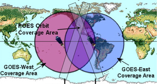
Even though infrared measurements of LST from a satellite are possible only for cloudless sky, such monitoring is an important component of the GOES satellites observational program (Schmit et al. 2005). GOES system consists of one satellite operating as GOES-East (GOES-E) in the eastern part of the constellation at 75° west longitude, and one satellite operating as GOES-West (GOES-W) at 135° west longitude, furnishing half-hourly measurements over the hemisphere. Several investigators have studied operational LST algorithms for GOES Imagers (Sun and Pinker 2003; Sun, Pinker, and Basara 2004; Pinker et al. 2009; Yu et al. 2009), some efforts has been made to compare LSTs from different satellite sensors (Trigo et al. 2008; Jimenez-Munoz and Sobrino 2008; Inamdar et al. 2008; Zakšek and Oštir 2012); however, no effort has been made on the comparison of LST retrievals from GOES and polar-orbiting sensors. Furthermore, LST products from polar-orbiting satellites, such as MODerate resolution Imaging Spectroradiometer (MODIS), can be used to evaluate and mutually optimize LSTs from GOES-East and GOES-West over the coincident areas (Figure 1). With the growing demand for accurate and high-resolution LST inputs for weather forecasts and data assimilation models, as well as a long-term time series or climate data record (CDR) of consistent LST over large areas (Jin and Dickinson 2002), it is necessary to perform comparisons of LSTs derived from different satellites, to ensure the correct use and consistency of estimated parameters.

Figure 1. Sample figure of common area observed by GOES-West (GOES-W), GOES-East (GOES-E), and Polar-orbiting Operational Environmental Satellites (POES).

LST is highly variable in space and time (Olesen, Kind, and Reutter 1995). This paper will mainly focus on a case study in April 2004 for investigating the differences in LSTs derived from the imager onboard the GOES-West (GOES-10), GOES-East (GOES-12), and the MODIS onboard the Earth Observing System (EOS) over their collocated areas, discussing their thermal discrepancies caused by potential factors such as angular anisotropy and land surface properties (Barroso et al. 2005; Pinheiro et al. 2006; Trigo et al. 2008; Vinnikov et al. 2008). The date in April 2004 was selected as a case study, because at that period of time, GOES-West was GOES-10, which still included the classical split-window (SW) channels at 11 µm and 12 µm, and enabled us to compare the difference in dual-window algorithm and SW algorithm for the same sensor. However, the current GOES-West is GOES-15, which doesn't have the SW channels. Despite the complexity of evaluation, it is the only way to ensure the correct use of estimated parameters across different platforms.

GOES-M(12)-Q series has only one thermal window channel (11.0 µm) with the absence of 12.0 µm channel, so the conventional SW methodology that features correcting atmospheric effects (differential absorption) through radiation signal difference in two adjacent channels (McMillin 1975) cannot be used. In this study, a modified dual-window algorithm that combines middle-infrared 3.9 µm channel with infrared 11.0 µm channel to derive LST from GOES-West and GOES-East during April 2004 is used as a case study for comparison. Meanwhile, the GOES-West at that period of time was GOES-10 and still had the two SW thermal channels, and enabled us to compare LSTs derived from GOES-West with both of dual-window (3.9 + 11.0 µm) and SW (11.0 + 12.0 µm) algorithms. The methodology and data used are briefly described in Section II. Section III discusses the results, and conclusions are provided in Section IV.

2. Data and methodology

2.1. LST derivation from GOES

Theoretically, LST can be retrieved from at-sensor brightness temperature (BT) by transformation of the first-order Taylor-series linearization of the Planck function, a part of the complicated radiative transfer equation (RTE) in thermal infrared spectral bands:

Under clear sky conditions, the outgoing spectral radiance at the top of the atmosphere can be represented as:

(1)

where ε₀ is the surface spectral emissivity, B is the Plank function, τ₀ is the transmittance at the Earth's surface, R_a is the thermal path radiance, R_s is the path radiance resulting from scattering of solar radiation, R_d is the solar diffuse radiation, and R_r is the solar radiation and atmospheric thermal radiation reflected by the surface. T_s is the skin temperature, λ is the wavelength, µ = cos(θ), µ₀ = cos (θ_s), where θ is the satellite zenith angle, θ_s is the solar zenith angle, and φ_o is the azimuth angle.

The GOES observation data were obtained from the NOAA's Comprehensive Large Array-data Stewardship System (CLASS) (http://www.class.ngdc.noaa.gov/saa/products/welcome). After radiometric calibration and georeferencing, the original GOES-East and GOES-West raw data are converted to BT and re-projected to a regular 0.05 × 0.05 grid with half-hourly temporal frequency. The cloud mask from the GOES Surface and Insolation Product (GSIP) source dataset, provided by the GSIP product developer Dr. Istvan Laszlo, is used for all cloud detection. LST retrieval in each scanning mode is performed on each cloudless (i.e. ‘clear’ and ‘possible clear’ indicated by the cloud mask) land surface pixel, for day and night. The surface spectral emissivities needed for the derivation of LST are obtained from daily MODIS LST/Emissivity products derived from a physical-based day/night algorithm (Wan and Li 1997).

2.1.1. Dual-window (3.9 µm + 11.0 µm) LST algorithm

Due to the lack of split window on GOES-M (12)-Q series satellites, Sun, Pinker, and Basara (2004) developed a new LST algorithm by using the middle infrared (MIR) channel (3.9 µm), which shows less atmospheric absorption and attenuation than SW channels (11 and 12 µm) (May 1993; Sun and Pinker 2003). However, the MIR channel contains solar contamination during daytime, so a solar correction item that is based on the cosine function of solar zenith angle and BT at the MIR channel (cos θ_s × T_3.9) is added for daytime LST retrieval. In this study, this algorithm with some modification with explicit use of surface emissivity is adapted to retrieve LST from GOES-East and GOES-West.

Daytime:

(2)

Nighttime:

(3)

where θ is the satellite zenith angle, θ_s is the solar zenith angle, T₁₁ and T_3.9 are BT measured by GOES channels centered at 11.0 µm and 3.9 µm, respectively, ε is the mean effective emissivity , Δε is spectral emissivity difference (here ε₁₁, ε_3.9 is 11.0 µm and 3.9 µm, respectively). Coefficients (a₀, a₁, …, a₆, a₇) are obtained from the radiative transfer model simulations, which will be described in a later section.

2.1.2. SW LST algorithm

In order to compare LSTs derived from different algorithms on the same sensor, the widely used splint-window (SW) algorithm is selected for comparison. For the two adjacent channels (11 and 12 µm), SW technique has been widely used due to its simplicity and robustness, as well as accuracy improvement to single-channel method. SW algorithm assumes that LST can be obtained through a semi-empirical regression of simultaneous at-sensor BT measurements, where the atmospheric correction is a function of the differential absorption in the two SW channels and channel surface emissivities are known a priori (McMillin 1975; Wan and Dozier 1996).

A variety of SW algorithms (Price 1984; Ulivieri and Cannizzaro 1985; Becker and Li 1990; Prata 1993; Sobrino et al. 1994; Wan and Dozier 1996; Coll and Caselles 1997) have been developed to obtain LST from space. Among these, the well-known generalized SW (GSW) algorithm (Becker and Li 1990; Wan and Dozier 1996) is adapted to retrieve LST from GOES-West, given as:

(4)

where θ is the satellite zenith angle, , ε represents surface emissivity, T is BT, subscripts 11 and 12 refer to channels centered at 11.0 µm and 12 µm respectively, and a₀, a₁, …, a₇ are the regression coefficients automatically stratified under different conditions from the training with regression tree technique (Sun et al. 2013). This SW algorithm will only be applied to GOES-West (GOES-10 in 2004) in this study.

In both LST algorithms, a path correction term rectifying additional atmospheric attenuation as a function of satellite zenith angle (e.g. the last term in Equation 4) is added into the mathematical formula. This is because of the fact that the atmospheric path length at 60° of the satellite zenith angle is about two times larger than that at the nadir, where atmospheric absorption impacted by path water vapor may be amplified, which can significantly degrade the algorithm accuracy (McClain, Pichel, and Walton 1985; Yu, Privette, and Pinheiro 2008).

2.1.3. Forward simulations

To derive regression coefficients that relate LST as a function of satellite observed clear-sky at-sensor BTs, the MODTRAN4.3 (MODerate resolution atmospheric TRANsmission) radiative transfer model is used to perform forward simulations for GOES infrared channels and generate a simulation database. With the purpose of making simulations applicable to all possible (atmospheric/environmental) conditions, the atmospheric profiles with the matched surface height, pressure, temperature, and relative humidity from the global NCEP Reanalysis (NRA) with 17 vertical layers at 2.5° resolution (144 × 73) are used as inputs, covering a column water vapor (CWV) range from 0.0 to 7.0 g/cm² and a surface-air temperature difference range of −36.1 ∼ 30.0 K/°C.

Spectral response functions of the instruments are sensor-dependent. Upon simulating the outgoing radiances at the Top of Atmosphere (TOA) over a wide spectral range from 0.3 to 15 µm, we convolute over the spectral radiances with the response function of this specific instrument.

(5)

where L(λ) is the response function of the satellite, [λ₁, λ₂] is the wavelength range of a spectral channel.

As for another prerequisite parameter needed in simulations, surface emissivity, we define 18 different land surface types matching with the MODIS 17 IGBP types, plus one surface type Tundra as recommended by the JCSDA (Joint Center for Satellite Data Assimilation), to prescribe the unique surface emissivity values, which are employed from a spectral library of surface emissivity and reflectivity over a wide range of spectral wavelengths from the MODIS4.3 dataset (Cornette et al. 1994), and interpolated with filter response function at each appropriate emissivity spectrum.

Besides considering the effects of GOES view angular variation, dry/moist (cold/warm) atmosphere status, etc., simulations are stratified for: (1) 5 view zenith angle bins (0°, 2°, 4°, 6°, 8°, Table 1); (2) atmospheric CWV is categorized according to intervals of 0.5 cm: 1) ‘cold’ atmospheres, where the surface air temperature T_air is lower than 280 K; and 2) ‘warm’ atmospheres, where T_air is higher than 280 K; (3) day/night is separated using solar zenith angle θ_s (θ_s ≤ 85° is daytime, and θ_s > 85° is nighttime); (4) the atmospheric temperature profiles are aggregated according to the 11-µm BT, T₁₁ ≤ 280 K or 280 K, or T_air −15K < LST < T_air + 15 K with a 1 K increment. The ±15-K difference range includes most, but not all (e.g. some semiarid environments in some situations), conditions in nature. Then coefficients in Equations (2), (3), (4) are calculated with statistical fits from the complete simulation database.

Table 1. Zenith angle bins.

Zenith angle bin	1	2	3	4	5
Viewing zenith angle (VZA)	0°	2°	4°	6°	8°
Equal satellite zenith angle (SZA)	0°	12.8°	26.38°	41.75°	62.44°

2.2. MODIS LST product

The MODIS/Terra level 3 Daily LST/Emissivity products (Collection 005, shortname: MOD11C1) includes a pair of daytime and nighttime LST observations; configuring on a 0.05° geographic climate modeling grid (CMG) was used to compare with GOES LSTs. To match up the MODIS LST, GOES-East and GOES-West LSTs were re-projected to the same regular 0.05 × 0.05 grid. This product is produced using a physical-based day/night algorithm, which simultaneously retrieves surface spectral emissivities in seven thermal infrared bands (bands 20: 3.660–3.840 µm, 22: 3.929–3.989 µm, 23: 4.020–4.080 µm, 26: 1.360–1.390 µm, 29: 8.400–8.700 µm, 31: 10.780–11.280 µm, 32: 11.770–12.270 µm, 33: 13.185–13.485 µm) and LST from day/night pairs of MODIS data (Wan and Li 1997). Although cloud-contaminated LSTs have been removed with cloud mask (MOD35) (Ackerman et al. 1998) by a double-screening method to this product, we stick to use pixels with high-rank quality control flag, and consequently, all the MODIS pixels flagged with a poor confidence level are rejected. MODIS LST products have been widely used and evaluated as good quality datasets (Wang, Liang, and Meyers 2008; Coll, Wan, and Galve 2009; Li et al. 2014). We here use it mainly as polar-orbiting LST for comparison with GOES LST.

2.3. In situ observations

GOES and MODIS LST are also evaluated against in situ observations at Surface Radiation Budget Network (SURFRAD) sites. These sites strictly abide by the following rules: (1) site is far away from irrigated areas, lakes, and forests, and land surface should be as flat as possible, thus just minimizing heterogeneity and avoiding heterogeneous topography causing additional geometric distortions in satellite image pixels; (2) physical characteristics of a site should be representative of a large area, covered by crops or grass, correspondingly, surface emissivity is consistently high; (3) a minimum of obstructions that impede wind flow at the site; (4) observations should be carried out continuously, preferably long time series and high temporal resolution, affording sufficient data for validation and evaluation.

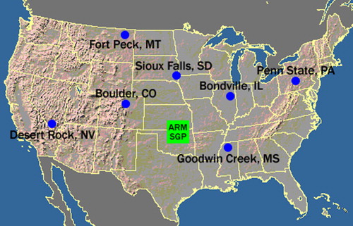
The SURFRAD network consists of 7 stations at present and was established in 1993 through the support of NOAA's Office of Global Programs, whose primary objective is to support climate research with accurate, continuous, long-term measurements pertaining to the surface radiation budget over the United States. Figure 2 shows the locations of the 7 SURFRAD stations. The quality-controlled SURFRAD data are available in daily files, which are distributed in near-real-time (http://www.esrl.noaa.gov/gmd/grad/surfrad/), including upwelling and downwelling solar and infrared radiative fluxes measured by a pyrgeometer/precision infrared radiometer measurements that is sensitive to the spectral range from 3.0 to 50 µm equipped on 10-m high tower. Since it is related to surface long-wave radiation by the Stefan-Boltzmann law, surface skin temperature can be converted as follows:

(6)

(7)

Figure 2. The locations of the seven SURFRAD sites.

where L^↑ is the SURFRAD observed upwelling long-wave radiation, L^↑ is the atmospheric downwelling long-wave radiation at the surface, σ is the Stefan-Boltzmann's constant (5.67 × 10–8 W m⁻² K⁻⁴), and ε_b is surface broadband emissivity over the entire infrared region, which can be estimated by MODIS narrowband emissivity (ε₂₉, ε₃₁, ε₃₂) at band 29 (8.400–8.700 µm), 31 (10.780–11.280 µm), and 32 (11.770–12.270 µm) derived from MODIS day/night LST algorithm (Wang et al. 2005):

(8)

3. Results

3.1. Inter-comparison of LST from GOES and MODIS

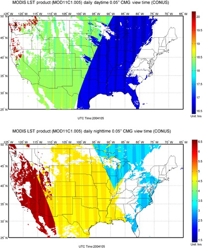
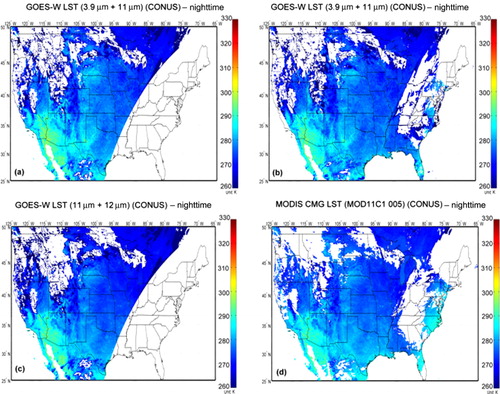
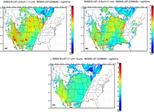
It is well-known that GOES imager takes about 20 minutes to scan the full disk, while for polar orbiting system, like MODIS, there is about 102-minute time difference between two different passes. Figure 3 demonstrates the distribution of observation times of MODIS over the continental United States (CONUS) during daytime and nighttime. Since LST varies with time, so time difference between GOES and MODIS will definitely induce LST differences. We therefore generated LST composite from GOES according to MODIS viewing time in a similar way to MODIS daily composite product. As shown in Figure 4, during daytime, the LST differences between GOES and MODIS show high spatial variations. In general, differences in LSTs between GOES-East with dual-window algorithm (LST_3.9µm+11µm) and MODIS vary in the range of 2 K to 8K. Differences in LSTs between GOES-West with dual-window algorithm (LST_3.9µm+11µm) and MODIS vary from 0 K to 6K. Meanwhile, LST differences between GOES-West with SW algorithm (LST_11µm+12µm) and MODIS vary from −6 K to 2 K (Figure 5). During nighttime, LST differences between GOES-East with dual-window algorithm and MODIS (GOES-East LST_3.9µm+11µm – MODIS LST) are mostly within 0 K to 3 K, differences in GOES-West LST_3.9µm+11µm and MODIS LST are mostly within 0 K to 4 K, LST differences between GOES-West with SW algorithm and MODIS (GOES-West LST_11µm+12µm – MODIS) are mostly within −2 K to 0 K (Figures 6 and 7). It is particularly evident that LST discrepancies between GOES and MODIS during nighttime (Figure 7) are smaller than those during daytime (Figure 5).

Figure 3. Terra/MODIS viewing time in UTC during day (upper) and night (lower) on 14 April 2004.

Figure 4. (a) GOES-W (3.9 + 11 µm), (b) GOES-E (3.9 + 11 µm), (c) GOES-W (11 + 12 µm), and (d) MODIS LST for daytime composite according to MODIS viewing time on 14 April 2004.

Figure 5. (a) GOES-W (3.9 + 11 µm)-MODIS, (b) GOES-E (3.9 + 11 µm)-MODIS, and (c) GOES-W (11 + 11 µm)-MODIS during daytime.

Figure 6. (a) GOES-W (3.9 + 11 µm), (b) GOES-E (3.9 + 11 µm), (c) GOES-W (11 + 12 µm), and (d) MODIS LST for nighttime composite according to MODIS viewing time on 14 April 2004.

Figure 7. (a) GOES-W (3.9 + 11 µm)–MODIS, (b) GOES-E (3.9 + 11 µm)–MODIS, and (c) GOES-W (11 + 11 µm)–MODIS during nighttime.

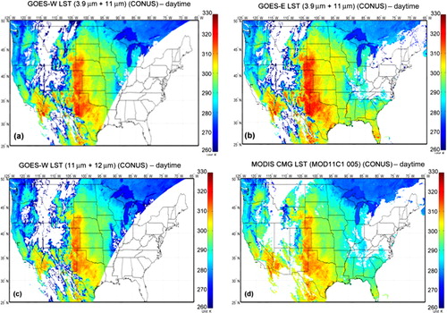
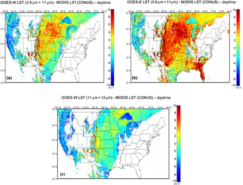
We can summarize the following general patterns: for dual-window (3.9 µm + 11 µm) algorithm, both GOES-East and GOES-West LST values tend to be warmer than the MODIS LSTs. While for the SW (11 µm + 12 µm) algorithm, GOES-West LST values are close to the MODIS LSTs. This is because the solar contamination in the middle-infrared (3.9 µm) channel, which includes solar radiation reflected by the Earth's surface during daytime, makes the BT at the 3.9 µm channel increase; therefore, LST values increase during daytime.

In general, the Root Mean Square (RMS) errors from the dual-window algorithm are bigger than that from the SW algorithm and MODIS LSTs, while the LST error from the GOES with the SW algorithm is close to that from the MODIS. Jimenez-Munoz and Sobrino (2008) also commented the increase on the LST error on GOES 12 and 13 because of the change in the second TIR band, from 12 to 13 µm, compared to the classical SW in GOES 8, 9, 10, 11. Nevertheless, the RMS errors from the GOES-West (2.15 K) and GOES-East (2.17 K) show no big difference with the same dual-window algorithm.

What factors may cause the differences across different platforms? Trigo et al. (2008) compared the LST products from the SEVIRI and MODIS, and found the differences are impacted by the satellite viewing angle differences, surface orography, and surface type. In the study of Trigo et al. (2008), both SEVIRI LST and MODIS LST used the same generalized SW algorithm. While in our study, two different algorithms, dual-window and SW algorithms, are used. We can see LST from the GOES-West with SW algorithm shows no significant difference from MODIS LST, meanwhile, even for the same instrument, like the GOES-West, different algorithms, such as the dual-window and SW algorithms here, demonstrate significant difference, especially during daytime.

3.2. Comparison of dual-window and SW algorithms for LST retrieval from GOES-West

From the above analysis, in addition to the time difference, we can see the difference between dual-window and SW algorithms played important role in the LST differences between GOES and MODIS. Therefore, it is appropriate to examine whether the LST retrieved from the dual-window (3.9 µm + 11 µm) algorithm is comparable to LST retrieved from the SW (11 µm +12 µm) algorithm, to ensure the applicability of LSTs from the dual-window algorithm or LST_3.9µm+11µm in the future. The performances of the two algorithms are assessed by sensitivity and algorithm accuracy analyses.

3.2.1. Sensitivity analysis

To further analyze the mismatches between GOES and MODIS LST products, the GOES-West LST differences between dual-window and SW algorithms are analyzed in terms of (1) satellite viewing angle (SVA), (2) vegetation over, (3) surface emissivity, and (4) surface type. Figure 7 displays the mean differences between the dual-window (3.9 µm + 11 µm) and SW (11 µm + 12 µm) LST algorithms against satellite viewing angles and surface properties, such as the vegetation cover or fraction (f) and surface emissivity at MIR 3.9 µm and IR 11 µm, for the whole continental US. As expected, the difference in LSTs between the dual-window and the SW algorithms is very sensitive to these parameters (Figure 8). The difference increases with satellite viewing angles. For daytime (left column), the difference between the LSTs decreases with increasing vegetation cover and emissivity at 3.9 µm. This may be because surfaces with high vegetation cover are more homogeneous and the uncertainty on emissivity is low. If the vegetation fraction is less than 0.4, the difference can be above 2 K/°C. While surface emissivity at MIR channel played the most remarkable role, if the 3.9 µm emissivity is below 0.80, the difference can be beyond 10 K/°C. The emissivity at MIR for some barren surfaces may be below 0.8, and crop regions may also undergo significant changes in surface emissivity following vegetation growth, decay, and harvesting. Similar to surface emissivity, the difference also depends on land use or land cover types (not shown). For example, evergreen broadleaf forest has the smallest difference with negative values, while desert or savannas has the largest difference with higher positive values, highlighting the strong temperature contrasts between dense vegetation and barren or sparsely vegetated ground.

Figure 8. GOES-W LST difference between dual-window (3.9 µm + 11 µm) and SW (11 µm +12 µm) algorithms against classified satellite viewing angle and surface properties (vegetation fraction and emissivity).

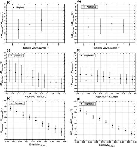
Moreover, for daytime/nighttime comparison, the difference is significantly smaller during nighttime, which indicates that nighttime difference is much less influenced by the viewing geometry and surface properties, as compared to daytime period. This indicates that nighttime LST is less influenced by algorithm difference.

Because surface thermal property is fairly stable and homogeneous during nighttime, nighttime LST retrieval errors are less sensitive to a variety of factors such as viewing geometry and surface properties. While during daytime, surface thermal property shows high variability, which plays roles in conjunction with satellite viewing geometry and vegetation coverage. Moreover, different channels/algorithms or sensors may have different responses to these properties, especially surface emissivity at MIR channel with high variability and low values below 0.8 for some barren surface types, resulting in inconsistent and bigger difference range during daytime. Since SW algorithm is used to derive LST from GOES 8–11, the dual-window algorithm is used for GOES (12)-Q. In order to develop consistent LST products from all the GOES series satellites, it is essential to correct the effects of viewing geometry, especially surface properties, for daytime LST retrieval, while it is better to use night scenes for the assessment of possible biases between algorithms/sensors.

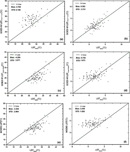
3.2.2. Algorithm accuracy

For each of the two algorithms, we calculated the Bias, standard deviation (STD), and RMS between satellite-derived LST and in situ observations referred to as ground-truth LST (Figure 9). The scatter plots (Figure 9) indicate that the dual-window (3.9 µm + 11 µm) algorithm overestimates LST with bias 2.7 K/°C during daytime, but performs well with bias close to zero as 0.36 K/°C during nighttime. Meanwhile the SW algorithm underestimates LST with bias −4.29 K/°C during daytime, and slightly overestimates LST with bias 0.76 K/°C during nighttime. The MODIS product demonstrates similar results to the SW algorithm, underestimates LST with bias −3.3 K/°C during daytime, but overestimates LST with bias 2.43 K/°C during nighttime. In general, during nighttime, the bias errors (accuracy) from GOES LSTs are less (better) than the MODIS LST, but the standard deviation (STD) errors (precision) are larger (worse) than the MODIS LSTs. For all-day evaluations (figure not shown), dual-window algorithm shows worse performance than the SW (11 µm + 12 µm) algorithm, yielding STD of 2.36 K from the dual-window algorithm, compared to STD of 1.83 K from the SW algorithm.

Figure 9. Scatter plots of LST derived from the GOES-W with dual window algorithm (a, b), and SW (c, d), and MODIS LST (e, f) versus in-situ observations during daytime (left column) and nighttime (right column) on 14 April 2004.

In general, all of the accuracy comparisons show that using the dual-window algorithm to derive LST is fairly feasible, although its total accuracy is slightly worse than that of the SW algorithm. Meanwhile, the result indicates that the lack of SW channel on the GOES M (12)-Q era may degrade the performance of LST retrieval.

4. Summary and conclusions

In this study, differences in LST across different platforms were investigated. Due to the lack of SW channels on the GOES-M (12)-Q era, a dual-window algorithm, which combines the mid-infrared 3.9 µm channel with less atmospheric absorption than the infrared 11 µm channel, was applied to derive LST from both GOES-East and GOES-West. Meanwhile, GOES-West (10) has the two SW thermal channels, and enables us to compare LSTs derived with the dual-window and SW algorithms. The LSTs derived from GOES-East and GOES-West were also compared to MODIS LSTs and evaluated against ground observations. The results can be summarized below:

1. During daytime, LSTs derived from GOES with the dual-window algorithms are warmer than MODIS LSTs; meanwhile, LSTs derived from GOES-West with SW algorithm are close to MODIS LST. During nighttime, GOES LSTs from both dual-window and SW algorithms show no big difference from MODIS LSTs.

2. The difference in LSTs across different platforms during daytime may be mostly caused by the difference in dual-window and SW algorithms. It is found the LST difference between dual-window and SW algorithms is affected by anisotropic effect, especially surface properties, such as vegetation cover and/or surface emissivity at the mid-infrared channel.

3. When evaluate against the in situ observations, during daytime, dual-window algorithm overestimates LST, while SW algorithm underestimates. During nighttime, both algorithms work well.

4. All day evaluations against the ground truth show, in general, LSTs derived from the dual-window algorithm are usually larger than those from SW algorithm. This indicates the lack of SW channels during the GOES M (12)-Q era may degrade the performance of LST retrievals.

Acknowledgments

The authors thank three anonymous reviewers for their helpful comments and suggestions that have significantly improved this article. We also appreciate the editors for their help and contribution to the society. The manuscript contents are solely the opinions of the authors and do not constitute a statement of policy, decision, or position on behalf of NOAA or the US Government.

Funding

This work was supported by NOAA PSDI program (NA11NES4400012), and Chinese Academy of Sciences/State Administration of Foreign Experts Affairs (CAS/SAFEA) International Partnership Program (KZZD-EW-TZ-09).

Additional information

Funding

Funding: This work was supported by NOAA PSDI program (NA11NES4400012), and Chinese Academy of Sciences/State Administration of Foreign Experts Affairs (CAS/SAFEA) International Partnership Program (KZZD-EW-TZ-09).

References

- Ackerman, S. A., K. I. Strabala, W. P. Menzel, R. A. Frey, C. C. Moeller, and L. E. Gumley. 1998. “Discriminating Clear Sky from Clouds with MODIS.” Journal of Geophysical Research 103 (24): 32141–32157. doi:10.1029/1998JD200032.
- Barroso, C., I. F. Trigo, F. Olesen, C. DaCamara, and M. P. Queluz. 2005. “Intercalibration of NOAA and Meteosat Window Channel Brightness Temperatures.” International Journal of Remote Sensing 26: 3717–3733. doi:10.1080/01431160500159834.
- Becker, F., and Z.-L. Li. 1990. “Towards a Local Split-Window Method Over Land Surfaces.” International Journal of Remote Sensing 11 (3): 369–393. doi:10.1080/01431169008955028.
- Coll, C., and V. Caselles. 1997. “A Split-Window Algorithm for Land Surface Temperature from Advanced very High Resolution Radiometer Data: Validation and Algorithm Comparison.” Journal of Geophysical Research 102 (14): 16697–16713. doi:10.1029/97JD00929.
- Coll, C., Z. Wan, and J. M. Galve. 2009. “Temperature-Based and Radiance-Based Validation for the V5 MODIS Land-Surface Temperature Product.” Journal of Geophysical Research 114: D20102. doi:10.1029/2009JD012038.
- Cornette, W. M., P. K. Acharya, D. C. Robertson, and G. P. Anderson. 1994. Moderate Spectral Atmospheric Radiance and Transmittance Code (MOSART). Report R-057-94 (11–30). La Jolla, CA: Photon Research Associates.
- Dickinson, R. E. 1996. “Land Surface Processes and Climate Modeling.” Bulletin of American Meteorological Society 76: 1445–1448.
- Inamdar, A. K., A. French, S. Hook, G. Vaughan, and W. Luckett. 2008. “Land Surface Temperature (LST) Retrieval at High Spatial and Temporal Resolutions over the Southwestern US.” Journal of Geophysical Research 113 (7): D07 107. doi:10.1029/2007JD009048.
- Jiang, G.-M., and Z.-L. Li. 2008. “Split-Window Algorithm for Land Surface Temperature Estimation from MSG1-SEVIRI Data.” International Journal of Remote Sensing 29 (20): 6067–6074. doi:10.1080/01431160802235860.
- Jimenez-Munoz, J. C., and J. A. Sobrino. 2008. “Split-Window Coefficients for Land Surface Temperature Retrieval from Low-Resolution Thermal Infrared Sensors.” IEEE geoscience and remote sensing letters 5 (4): 806–809. doi:10.1109/LGRS.2008.2001636.
- Jimenez-Munoz, J. C., J. A. Sobrino, C. Mattar, G. Hulley, and F. M. Gottsche. 2014. “Temperature and Emissivity Separation from MSG/SEVIRI Data.” IEEE Transactions on Geoscience and Remote Sensing PP (99): 1–15. doi:10.1109/TGRS.2013.2293791.
- Jin, M., and R. E. Dickinson. 2002. “New Observational Evidence for Global Warming from Satellite Data Set.” Geophysical Research Letters 29 (10): 39-1–39-4. doi:10.1029/2001GL013833.
- Jin, M., R. E. Dickinson, and D. L. Zhang. 2005. “The Footprint of Urban Areas on Global Climate as Characterized by MODIS.” Journal of Climate 18 (10): 1551–1565. doi:10.1175/JCLI3334.1.
- Li, S., Y. Yu, D. Sun, D. Tarpley, X. Zhasn, and L. Chiu. 2014. “Evaluation of 10 Year AQUA/MODIS Land Surface Temperature with SURFRAD Observations.” International Journal of Remote Sensing 35: 830–856. doi:10.1080/01431161.2013.873149.
- Liang, S. 2001. “An Optimization Algorithm for Separating Land Surface Temperature and Emissivity from Multispectral Thermal Infrared Imagery.” IEEE Transactions on Geoscience and Remote Sensing 39: 264–274. doi:10.1109/36.905234.
- May, D. A. 1993. “Global and Regional Comparative Performance of Linear and Non-Linear Satellite Multichannel Sea Surface Temperature Algorithms.” Tech. Rep. NRL/MR/7240-93-7049, Naval Research Laboratory, Washington, DC, 36 p.
- McClain, E. P., W. G. Pichel, and C. C. Walton. 1985. “Comparative Performance of AVHRR-Based Multichannel Sea Surface Temperatures.” Journal of Geophysical Research 90 (6): 11587–11601. doi:10.1029/JC090iC06p11587.
- McMillin, L. M. 1975. “Estimation of Sea Surface Temperatures from Two Infrared Window Measurements with Different Absorption.” Journal of Geophysical Research 80 (36): 5113–5117. doi:10.1029/JC080i036p05113.
- Olesen, F.-S., O. Kind, and H. Reutter. 1995. “High Resolution Time Series of IR Data from a Combination of AVHRR and METEOSAT.” Advances in Space Research 16 (10): 141–146. doi:10.1016/0273-1177(95)00394-T.
- Park, S., J. J. Feddema, and S. L. Egbert. 2005. “MODIS Land Surface Temperature Composite Data and their Relationships with Climatic Water Budget Factors in the Central Great Plains.” International Journal of Remote Sensing 26 (6): 1127–1144. doi:10.1080/01431160512331326503.
- Pinheiro, A. C. T., R. Mahoney, J. L. Privette, and C. J. Tucker. 2006. “Development of a Daily Long Term Record of NOAA-14 AVHRR Land Surface Temperature over Africa.” Remote Sensing of Environment 103: 153–164. doi:10.1016/j.rse.2006.03.009.
- Pinker, R. T., D. Sun, M.-P. Hung, C. Li, and J. B. Basara. 2009. “Evaluation of Satellite Estimates of Land Surface Temperature from GOES over the United States.” Journal of Applied Meteorology 48: 167–180. doi:10.1175/2008JAMC1781.1.
- Prata, A. J. 1993. “Land Surface Temperature Derived from the Advanced Very High Resolution Radiometer and the Along-Track Scanning Radiometer: 1. Theory.” Journal of Geophysical Research 98 (9): 16689–16702. doi:10.1029/93JD01206.
- Price, J. C. 1984. “Land Surface Temperature Measurements form the Split Window Channels of theNOAA-7/AVHRR.” Journal of Geophysical Research 89 (5): 7231–7237. doi:10.1029/JD089iD05p07231.
- Schmit, T. J., M. M. Gunshor, W. P. Menzel, J. J. Gurka, J. Li, and A. S. Bachmeir. 2005. “Introducing the Next Generation Advanced Baseline Imager on GOES-R.” Bulletin of American Meteorological Society 86: 1079–1096. doi:10.1175/BAMS-86-8-1079.
- Sellers, P. J., F. G. Hall, G. Asrar, D. E. Strebel, and R. E. Murphy. 1988. “The First ISLSCP Field Experiment (FIFE).” Bulletin of American Meteorological Society 69 (1): 22–27. doi:10.1175/1520-0477(1988)069<0022:TFIFE>2.0.CO;2.
- Sobrino, J. A., Z. L. Li, M. P. Stoll, and F. Becker. 1994. “Improvements in the Split Window Technique for Land Surface Temperature Determination.” IEEE Transactions on Geoscience and Remote Sensing 32: 243–253. doi:10.1109/36.295038.
- Sun, D., and R. T. Pinker. 2003. “Estimation of Land Surface Temperature from Geostationary Operational Environmental Satellite (GOES-8).” Journal of Geophysical Research 108: 4326. doi:10.1029/2002JD002422.
- Sun, D., and R. T. Pinker. 2007. “Retrieval of Surface Temperature from the MSG-SEVIRI Observations: Part I. Methodology.” International Journal of Remote Sensing 28 (23): 5255–5272. doi:10.1080/01431160701253246.
- Sun, D., R. T. Pinker, and J. B. Basara. 2004. “Land Surface Temperature Estimation from the Next Generation of Geostationary Operational Environmental Satellites: GOES M-Q.” Journal of Applied Meteorology 43: 363–372. doi:10.1175/1520-0450(2004)043%3C0363:LSTEFT%3E2.0.CO;2.
- Sun, D., R. T. Pinker, and M. Kafatos. 2006. “Diurnal Temperature Range over the United States: A Satellite View.” Geophysical Research Letters 33: L05705. doi:10.1029/2005GL025384.
- Sun, D., Y. Yu, L. Fang, and Y. Liu. 2013. “Towards an Operational Land Surface Temperature Algorithm for the GOES.” Journal of Applied Meteorology and Climatology 52: 1974–1986. doi:10.1175/JAMC-D-12-0132.1.
- Trigo, I. F., I. T. Monteiro, F. Olesen, and E. Kabsch. 2008. “An Assessment of Remotely Sensed Land Surface Temperature.” Journal of Geophysical Research 113: D17108. doi:10.1029/2008JD010035.
- Ulivieri, C., and G. Cannizzaro. 1985. “Land Surface Temperature Retrievals from Satellite Measurements.” Acta Astronautica 12 (12): 977–985. doi:10.1016/0094-5765(85)90026-8.
- Vinnikov, K. Y., Y. Yu, M. K. Rama Varna Raja, D. Tarpley, and M. Goldberg. 2008. “Diurnal-Seasonal and Weather-Related Variations of Land Surface Temperature Observed from Geostationary Satellites.” Geophysical Research Letters 35: L22708. doi:10.1029/2008GL035759.
- Wan, Z., and J. Dozier. 1996. “A Generalized Split-Window Algorithm for Retrieving Land Surface Temperature from Space.” IEEE Transactions on Geoscience and Remote Sensing 34 (4): 892–905. doi:10.1109/36.508406.
- Wan, Z., and Z.-L. Li. 1997. “A Physics-Based Algorithm for Retrieving Land-surface Emissivity and Temperature from EOS/MODIS Data.” IEEE Transactions on Geoscience and Remote Sensing 35(4): 980–996. doi:10.1109/36.602541.
- Wang, W., S. Liang, and T. Meyers. 2008. “Validating MODIS Land Surface Temperature Products Using Long-Term Nighttime Ground Measurements.” Remote Sensing of Environment 112 (3): 623–635. doi:10.1016/j.rse.2007.05.024.
- Wang, K., Z. Wan, P. Wang, M. Sparrow, J. Liu, X. Zhou, and S. Haginoya. 2005. “Estimation of Surface Long Wave Radiation and Broadband Emissivity Using Moderate Resolution Imaging Spectroradiometer (MODIS) Land Surface Temperature/Emissivity Products.” Journal of Geophysical Research 110: D11109. doi:10.1029/2004JD005566.
- Yu, Y., J. L. Privette, and A. C. Pinheiro. 2008. “Evaluation of Split Window Land Surface Temperature Algorithms for Climate Data Records.” IEEE Transactions on Geoscience and Remote Sensing 46 (1): 179–192. doi:10.1109/TGRS.2007.909097.
- Yu, Y., D. Tarpley, J. L. Privette, M. K. Rama Varna Raja, K. Vinnikov, and H. Xu. 2009. “Developing Algorithm for Operational GOES-R Land Surface Temperature Product.” IEEE Transactions on Geoscience and Remote Sensing 47 (3): 936–951. doi:10.1109/TGRS.2008.2006180.
- Zakšek, K., and K. Oštir. 2012. “Downscaling Land Surface Temperature for Urban Heat Island Diurnal Cycle Analysis.” Remote Sensing of Environment 117: 114–124. doi:10.1016/j.rse.2011.05.027.