Hexagonal connectivity maps for Digital Earth

Abstract

Geospatial data are gathered through a variety of different methods. The integration and handling of such datasets within a Digital Earth framework are very important in many aspects of science and engineering. One means of addressing these tasks is to use a Discrete Global Grid System and map points of the Earth's surface to cells. An indexing mechanism is needed to access the data and handle data queries within these cells. In this paper, we present a general hierarchical indexing mechanism for hexagonal cells resulting from the refinement of triangular spherical polyhedra representing the Earth. In this work, we establish a 2D hexagonal coordinate system and diamond-based hierarchies for hexagonal cells that enables efficient determination of hierarchical relationships for various hexagonal refinements and demonstrate its usefulness in Digital Earth frameworks.

Keywords:

• Digital Earth framework
• hexagonal subdivision
• indexing
• triangulation
• hierarchy
• multiresolution

1. Introduction

Digital Earth is a framework for the management and manipulation of geospatial data, spanning a multitude of scientific disciplines (Goodchild 2000). In this framework, data are assigned to locations and may be analyzed at multiple resolutions. Each resolution of this framework provides data with a specific level of detail. This multiresolution property is beneficial for efficient vector data and coverage-based data (Wartell et al. 2003). For practical purposes, the finest resolution is usually high enough such that cells with area in square millimeters can be supported.

One approach in assigning data to the Earth's positions is to discretize the globe into regions called cells. Cells then represent areas containing geospatial information associated with a point of interest. Several methods exist to partition the Earth. Latitude/longitude lines or Voronoi cells can be used to partition the Earth into regions of irregular size or shape (Chen, Zhao, and Li 2004; Faust et al. 2000). However, regular cells are often more desirable for a Digital Earth framework as they support efficient algorithms for handling important queries such as containment (which cell includes a point), neighborhood finding, and determining hierarchical relationships between cells (Sahr, White, and Kimerling 2003).

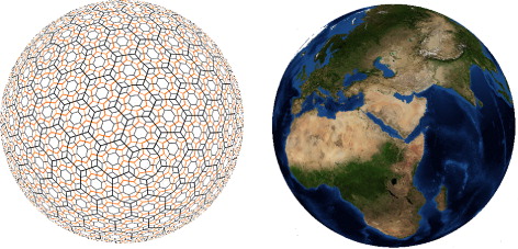
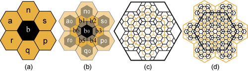
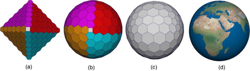
Discrete Global Grid Systems (DGGS) provide a representation of the Earth with mostly regular cells (Goodchild 2000; Sahr, White, and Kimerling 2003). The cells of DGGS may be triangular, quadrilateral (squares or diamonds), or hexagonal. Hexagonal cells are particularly desirable due to their unique characteristics, including uniform definition for adjacency and reduced quantization error (Sahr 2011; Snyder, Qi, and Sander 1999). Figure 1 illustrates the Earth partitioned using hexagonal cells.

Figure 1. Icosahedral Snyder equal area aperture 3 hexagonal grid (ISEA3H) (PYXIS Innovation 2014).

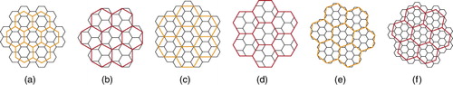
Six types of hexagonal refinement are mostly used throughout the literature: 1-to-3, 1-to-4, and 1-to-7 refinement in both their centroid-aligned and vertex-aligned variants (Figure 2). Centroid-aligned refinements (c-refinements) produce refined cells sharing centroids with coarse cells while vertex-aligned refinements (v-refinements) generate refined cells with vertices that are shared with the centroid of coarse cells. To generate multiple resolutions with regular spherical cells, a polyhedron is refined and its resulting faces are projected to the sphere by a spherical projection. Area preserving projections such as Snyder projections are especially preferable as they simplify data analysis on the Earth (Snyder 1992).

Figure 2. The c-refinements and v-refinements (shown in orange and red, respectively) for 1-to-3 refinement ((a), (b)), 1-to-4 refinement ((c), (d)), and 1-to-7 refinement ((e), (f)).

To associate information with cells at different levels of refinement, a data structure is required. Quadtrees (Samet 2005; Tobler and Chen 1986) are commonly used to support spatial queries for quad cells but require many pointers to establish connectivity between nodes, which reduces efficiency in high resolution applications with a large data load. To overcome this issue, several indexing methods have been developed for quadtrees. However, quadtrees and their indexing methods cannot be directly applied in the hexagonal case, due to the lack of congruency of hexagons. As a result, an indexing specifically designed for hexagonal cells or an adapting mechanism to benefit from simple congruent shape of quads is required that can efficiently support essential queries.

Existing hexagonal indexing methods primarily operate on a complicated fractal-like coverage hierarchy that makes the operations difficult to handle. They are also defined only for a specific type of refinement or polyhedron. In this paper, we introduce a general scheme for indexing hexagonal cells based on modifications of hexagonal coordinate systems. This indexing maintains the hierarchical relationships between successive resolutions. The proposed scheme is general and not dependent on a specific type of polyhedron or refinement, handling essential queries such as hierarchical traversal between cells and neighborhood finding in constant time. Instead of using fractal coverage hierarchies, we define two simple diamond-based hierarchical coverage for hexagons and demonstrate their usefulness for a Digital Earth framework through several example results.

As part of our method evaluation, we compare our indexing with PYXIS indexing (Peterson 2006; Vince and Zheng 2009). PYXIS indexing is from the same category of a set of hierarchical indexing methods designed for hexagonal cells that use a fractal hierarchical coverage (Sahr, White, and Kimerling 2003; Gibson and Lucas 1982).

We organize the paper as follows: Related work is presented in Section 2. The terminology of the paper is established in Section 3. Section 4 describes our comprehensive indexing method. Hierarchy is formally defined in Section 5, and two variations of hexagonal hierarchy as well as their benefits are also presented. In Section 6, we provide comparison and results. We describe a common hierarchical indexing method called PYXIS indexing and compare results with our method. We finally conclude in Section 7.

2. Related work

One way to represent the Earth is to use DGGS. These systems differ from each other based on the underlying polyhedron, type of cells, refinement, projection, and data structure employed. In the following, we provide some work related to each of these elements. For a complete survey, please refer to Goodchild (2000) and references therein.

2.1. Underlying polyhedra

Numerous polyhedra have been used to approximate the Earth. For instance, an octahedron can be projected to the sphere in such a way that each face corresponds to an octant of the latitude/longitude spherical coordinate system (White 2000). The tetrahedron has been used to represent the Earth in 3D engines that render a virtual globe due to its simplicity (Cozzi and Ring 2011). The truncated icosahedron better approximates the sphere (White, Kimerling, and Overton 1992). Note that the truncated icosahedron can be constructed by refining the regular icosahedron which itself is widely used as it induces less distortion as compared with other platonic solids (White, Kimerling, and Overton 1992). Therefore, the truncated icosahedron is also widely used for approximating the Earth (Fekete and Treinish 1990; Sahr 2008; White 2000; PYXIS Innovation 2014; Vince and Zheng 2009).

The cube is also an interesting polyhedron for spherical representation due to its adaptability to Cartesian coordinates, hardware devices and existing data structures such as quadtrees (Alborzi and Samet 2000; Mahdavi-Amiri, Bhojani, and Samavati 2013). The dodecahedron, which has 12 pentagonal faces, has been also used for Earth representation (Wickman, Elvers, and Edvarson 1974). However, since pentagon-to-pentagon refinement has not been defined, it is not a popular choice for hierarchical representation of the Earth.

2.2. Type of cells

Different shapes – such as hexagons, quads or triangles – can be used as cells for DGGS. For instance, Alborzi and Samet (2000) use quadrilateral faces of a refined cube while Dutton (1999) uses the triangular faces of an octahedron.

In this paper, we consider hexagonal cells. As discussed by Sahr (2011), this type of cell is preferred in many applications due to their uniform adjacency, regularity, and support for efficient sampling and smooth subdivision schemes (He and Jia 2005; Kamgar-Parsi, Kamgar-Parsi, and Sander 1989; Claes, Beets, and Van Reeth 2002). Although hexagonal cells may be the best choice for sampling the surface of the Earth, they need to be addressed and rendered efficiently. We use diamonds (unit squares in hexagonal coordinate systems) to efficiently address hexagons and show how to triangulate them for efficient rendering (White 2000).

2.3. Type of refinement

Refinements are used to make finer cells based on initial coarse cells. Refinements are widely used in subdivision surfaces to make smooth objects (see Cashman 2012 and references therein). They can also be used to construct more cells on the sphere by refining polyhedral faces. To show the generality of our approach, we use six types of hexagonal refinement: 1-to-3, 1-to-4, and 1-to-7 c-refinements and v-refinements (Figure 2). Each of these refinements features some benefits over the others. 1-to-3 refinement increases the number of faces at a lower rate compared to the other two. Under this refinement, more resolutions are produced under a fixed maximum number of faces and, therefore, enables a smoother transition between resolutions. For example, Sahr (2008) uses hexagonal 1-to-3 c-refinement on an icosahedron while Vince (2006) uses the same refinement on the octahedron. While other refinements introduce a rotation in the lattices of two successive resolutions (Ivrissimtzis, Dodgson, and Sabin 2004), hexagonal 1-to-4 refinement produces aligned lattices at all levels of resolution, simplifying hierarchical analysis (Sadourny, Arakawa, and Mintz 1968; Thuburn 1997; Tong et al. 2013). None of these six refinements create a congruent coverage for the hexagonal lattices, i.e. a coarse hexagon is not aggregated by an exact number of fine cells (Sahr 2011). However, 1-to-7 refinement covers the hexagonal coarse shape better than the others. As a result, there is growing interest in this type of refinement (Middleton and Sivaswamy 2005).

2.4. Data structure

Indexing methods proposed for hexagonal cells have their own advantages and limitations. Vince (2006) proposes an efficient indexing based on barycentric coordinates for a 1-to-3 hexagonal refinement of the octahedron by initially placing its vertices at coordinates (±1, 0, 0), (0, ±1; 0), and (0, 0, ±1). Throughout the resolutions, the barycenter of each cell is taken to be its index. This method has been modified for a 1-to-4 hexagonal refinement of the same polyhedron (Ben, Tong, and Chen 2010). However, both of these methods are designed for a specific polyhedron and refinement and their extension to other polyhedra is not straightforward, since the vertices of other polyhedra do not fall nicely on independent axes.

Alternatively, in Vince and Zheng (2009), PYXIS Innovation (2014), an approach is used to index hexagonal cells of an icosahedron similar to generalized balance ternary indexing (Gibson and Lucas 1982) (see Section 6.1.). In this method, the prefix of every fine resolution cell is the index of its parent. Sahr (2008) also uses a similar approach to PYXIS indexing. Sahr also suggests a pyramid indexing based on hexagonal coordinate systems similar to the methods proposed in Middleton and Sivaswamy (2005), Snyder, Qi, and Sander (1999), Sahr (2008), and Burt (1980). Pyramid indexing works well for single resolution applications but it is not developed for multiresolution cells resulting from an arbitrary hexagonal refinement. Moreover, the multiresolution described by Middleton and Sivaswamy (2005), Sahr (2008), and Vince and Zheng (2009) is based on a fractal coverage resulting from a particular definition of hierarchy or circularly aggregating cells. These fractal coverages, however, are hard to render and their neighborhood finding operations are expensive (see Section 6).

In this paper, we propose a hexagonal indexing to support both hierarchical traversal and neighborhood finding in constant time. Our proposed indexing is general to support various refinements and polyhedron. This indexing is derived by means of hexagonal coordinate system for a single resolution (Middleton and Sivaswamy 2005; Snyder, Qi, and Sander 1999). To define a hierarchical relationship among the indices of cells, we establish a mapping between the coordinates of two successive resolutions resulting from the employed hexagonal refinements. We also provide a diamonds-based hierarchical traversal that provides a full coverage for polyhedra with a simpler boundary in compared to common fractal-based coverages (Vince and Zheng 2009; Sahr 2008).

3. Basic idea and terminology

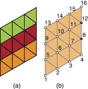
In this section, we explain the basic ideas and terminologies that we use throughout the paper. The surface of the Earth is represented by a spherical polyhedron in DGGS. As our hexagonal cells are created by simply refining triangular polyhedrons and taking the duality, we focus on triangular polyhedrons (icosahedron, octahedron, and tetrahedron). To work with these polyhedrons, we unfold them to simple diamond patterns within a 2D domain since our indexing method benefits from diamonds (see Figure 3). This pattern provides a mapping between 2D and 3D polyhedron since each triangular face of the polyhedron corresponds to a 2D triangle on the 2D pattern. Knowing this correspondence between 2D and 3D triangles, it is easy to map all points of these triangles using barycentric coordinates.

Figure 3. (a) An icosahedron (b) Unfolded icosahedron to a set of diamonds d_i. (c) Making hexagons by refining a diamond and applying duality.

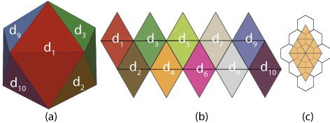
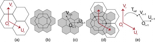
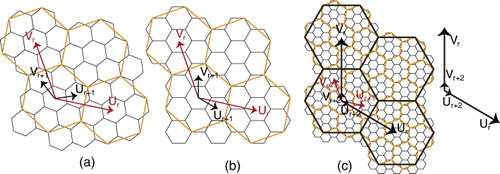
By using triangular refinements and taking the duality (e.g. replacing each face by a point and connecting the points whose correspondent faces are neighbors), initial hexagons are created (see Figure 3(c)). We can then use one of the six hexagonal refinements on the initial hexagons and create multiple resolutions. These hexagons are then projected to the sphere. Each hexagon on the 2D domain has a corresponding hexagonal face on the polyhedron and hexagonal cell on the sphere (see Figure 4).

Figure 4. (a) A red hexagon is shown on an unfolded tetrahedron. (b) The corresponding hexagonal face is drawn in red on a refined tetrahedron. (c) The corresponding cell is shown on a spherical tetrahedron.

A 2D lattice l is an array of points generated by a linear combination of two basis vectors U and V as with integer α and β. l is bounded when α and β are finite. Hexagons of each diamond form a 2D-bounded hexagonal lattice. To index these hexagons, we employ hexagonal integer coordinate systems that are compatible with the bounded lattice. A hexagonal coordinate system is defined as a triple in which O is the origin centered on an arbitrary hexagon and U and V are two unit length vectors with 120° difference.

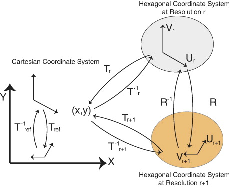
When a refinement is applied on a lattice to provide multiple resolutions, a set of new cells are produced. On these new cells, coordinate system is defined. If and are the coordinate system at resolution r and r + 1, respectively, transformation T_ref exists that transforms to . Using T_ref, we derive simple relationships between indices at multiple resolutions for various types of refinements. Using diamonds and these simple relationships, we establish two types of hierarchy that are beneficial to address essential queries.

Figure 5. (a) Triple (O_r, U_r, V_r) defines a coordinate system for resolution r. (b) 1-to-3 refinement is applied and resolution r + 1 is generated. (c) Triple (O_r+1, U_r+1, V_r+1) for resolution r + 1. (d) Two successive resolutions are overlayed. (e) T_ref maps (O_r, U_r, V_r) to (O_r+1, U_r+1, V_r+1).

4. Indexing hexagonal refinements

To assign data to cells and also address essential queries such as neighborhood finding, rendering, and retrieve data, we need a data structure. We use an indexing method obtained from hexagonal coordinate systems for this purpose. Given hexagonal coordinate systems , all hexagons get the integer coordinate of their centroid as their index, where their centroid is a units from O_r along U_r, and b units along V_r. Indices are always integer indicating the distance of the centroid of a hexagon to O_r along U_r and V_r Figure 5. When refinements are applied on hexagons, a set of new hexagons are created and indexed in the coordinate system (the transformed version of by T_ref.

Figure 6. (a) Hexagonal coordinate system and its associated indexing. (b) An unfolded octahedron and a hexagon falling in d ₁. (c) Diamond d(a,b) has its origin at (a,b) with axes aligned with the hexagonal coordinate system.

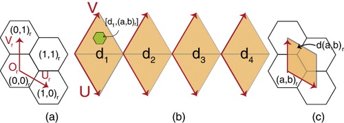
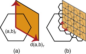
As discussed earlier, initial diamonds formed by pairing two triangles, are bounded lattices. These initial diamonds have coordinate systems aligned with the coordinate systems of hexagons at the first resolution. To distinguish between hexagons in different diamonds, we label each diamond by d_i and a hexagon lying in d_i at resolution r has index (Figure 6(b)). We can also define diamonds associated with each hexagon as quads with edges aligned to axes U_r and V_r of a hexagonal coordinate system (see Figure 6(c)). As a result, each hexagon is associated with a diamond with the same area and coordinate system.

4.1. Mapping resolutions

To traverse from a coarse resolution cell to a fine cell, a mechanism is needed that relates the successive resolutions. To achieve this, we determine the mapping R from indices of resolution r, to indices of resolutions r + 1. There exists a connection between T_ref and R as illustrated in Figure 7. We discuss more about the connection in this section.

Figure 7. Diagram illustrating hexagonal coordinate systems at successive resolutions and their connection to Cartesian coordinate systems.

To map the indices of a coarse resolution r to the fine indices of resolution r + 1, we use the basis transformation. For doing this, let and , has coordinate where . Note that we can also obtain R by mapping the hexagonal coordinates to the Cartesian coordinates. In fact, where T_r maps the hexagonal coordinates of resolution r to the Cartesian coordinates. Table 1 lists these matrices for 1-to-3 c-refinement when T_ref is composed of scaling and 30° rotation. Moreover, , therefore, choosing different T_ref affects and consequently affects R. In the following, we discuss how to generalize these equations to multiple resolutions and choose T_ref to simplify mapping R.

Table 1. Basis equality matrices for 1-to-3 c-refinement.

R	Tref	Tr	Tr+1

The matrix multiplication used to traverse between resolutions can be generalized for multiple resolutions and simplified to scalars. If is an index of a hexagon, it has index then 1-to-4 c-refinement, T_ref is simply a scaling by and R is just a scaling by two. As a result, Rⁿ is also a scaling by .

For other refinements, the form of R is not as clean as 1-to-4 refinement as R is not represented as a simple scaling. However, we can carefully define coordinate systems to simplify R. In 1-to-3 c-refinement, by taking even/odd resolutions coordinate systems aligned with even/odd resolutions, we can simplify traversing two resolutions to a scaling by three. This is due to the fact that , transforming coordinate system of even resolutions to odd is scaling and 30° rotation, and is composed of the same scaling with –30° rotation. Rotations of these transformations are canceled out and only a scaling is preserved (see Figure 8). These two transformations lead to two different R matrices called and corresponding to and , respectively. that map an index of an even/odd resolution r to an odd/even resolution r + 1 are listed in Table 2 (left).

Figure 8. (a) Hexagonal coordinate system and their Cartesian coordinates used to define T_r. (b) (O_r, U_r, V_r) are transformed by T_ref and new red coordinate system (O_r+1, U_r+1, V_r+1) is obtained. (1,0)_r and (0,1)_r have hexagonal coordinates (1,−1)_r+1 and (1,2)_r+1, respectively, in (O_r+1, U_r+1, V_r+1). (c) We can take coordinate system of (O_r+2, U_r+2, V_r+2) aligned with (O_r, U_r, V_r).

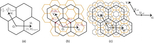
Table 2. Left: mappings for 1-to-3 refinement. Right: mapping for 1-to-7 refinement.

Refinement			R
1-to-3
Refinement	R +	R −	R
1-to-7

In 1-to-7 c-refinements, we cannot take aligned coordinate systems at every two successive resolutions and reduce mapping R to a scaling. This is due to 19° rotation of 1-to-7 refinement that is not canceled out after two resolutions. To simplify , we can consider where v_i are the eigenvectors of R. Therefore is simplified to where are corresponding eigenvalues to eigenvectors v_i. However, we can obtain even simpler mappings, if we switch between two versions of 1-to-7 refinements with 19° and –19° rotations (see Figure 9). If we alternate between these two refinements, R is simplified to scaling by 7. and corresponding to 1-to-7 refinements with 19° and –19°, respectively, are presented in Table 2 (right).

Figure 9. (a), (b) 1-to-7 refinement with 19° and –19° rotation. (c) Applying 1-to-7 refinement with 19° rotation followed by 1-to-7 refinement with –19° rotation. Note that it is possible to take aligned coordinate systems after two resolutions.

4.2. Mapping resolutions for v-refinements

If the set of centroids of all hexagons at resolution r is denoted by C^r, then under c-refinement, . This means a coordinate exists which indices the same location as . However, in v-refinements, the centroids of two successive resolutions are not aligned due to the translation in T_ref. As a result, and unlike c-refinements, we cannot choose the same origin for all resolutions. However, using a systematic predetermined location for the origins, we can calculate the locus of the origin at all resolutions.

In the 1-to-4and 1-to-7 v-refinement the lattices are aligned at every other resolution. As a result, we choose a fixed origin at the even and odd resolutions (see Figure 10(b) and (c)). However, for 1-to-3 refinement, lattices are never aligned. We choose for even r and for odd r as the origin of resolution r + 1 (Figure 10(a)). Using geometric series, we define a closed form for the origin of 1-to-3 refinement, discussed in more detail in Appendix A. Table 3 lists the origins of v-refinements at even and odd resolutions. This way, by defining coordinate systems at two successive resolutions, we define a simple mapping to traverse between resolutions both for c-refinements and v-refinements.

Figure 10. Origins of v-refinements at subsequent resolutions for (a) 1-to-3 (b) 1-to-4 and (c) 1-to-7 refinements. Fixed origins at odd and even resolutions are taken in (b) and (c).

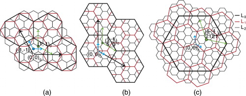
Table 3. Originsat resolution r + 1 for v-refinements at even and odd resolutions.

Refinement	Even	Odd
V 1-to-3
V 1-to-4	(0,0)0
V 1-to-7	(0,0)0

4.3. Reverse mapping

In addition to traversing from coarse resolutions to fine resolutions, mapping from a fine resolution cell to a coarse cell is also needed. A relation to traverse back through the resolutions and find a coarse hexagon is obtained by inverting the refinement matrix R. If we apply on arbitrary hexagon , it gives index in which a′ and b′ are not necessarily integers. To obtain a valid integer index at resolution r, we use the floor function . We will describe how this choice is compatible with our diamond-based hierarchy in the following section.

5. Hierarchy

From hexagonal refinement, a hierarchy can be defined. In defining hierarchy, each fine cell has exactly one corresponding coarse cell at any resolution except the coarsest. Formally, let S^r denote the set of n cells at resolution r, denote the cells of S^r, and denote the set of cells assigned to at resolution r + k. Every cell at resolution r + k has exactly one corresponding coarse cell at resolution r, hence and when . This way, we can define a hierarchical traversal query to find the set of all cells corresponding to a given cell , or determine the coarse cell corresponding to a given fine cell (i.e. ). In this paper, we provide two hierarchical coverage (congruent and incongruent) for hexagons which both benefit from diamonds.

5.1. Congruent hierarchy

It is possible to define a congruent hierarchy for diamonds. This means that a coarse diamond can be completely covered by a set of finer-scaled diamonds. This is the simplest type of hierarchy as the set of fine cells that are covered by a coarse diamond can be indexed in a simple range. For example, if a coarse diamond with index is refined n times by 1-to-4 refinement, the finer indices under have index where and . Using the corresponding diamond to each hexagon, we can define a similar hierarchy for hexagons.

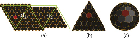
As discussed earlier, each hexagon has a corresponding diamond . We consider hexagon (where k is a positive integer) assigned to coarse hexagon if centroid of falls in diamond (see Figure 11). Since we have simplified the mappings to aligned coordinates handling by scalars, this diamond-based hierarchy is well defined for hexagons. Notice its boundary is also simpler than fractal coverage, therefore providing an efficient rendering, simple hierarchical relationships and neighborhood finding. Additionally, it supports mapping to other quad-based data structures as desired.

Figure 11. (a) Hexagon (a,b)_r and its corresponding diamond d(a,b)_r. (b) After two applications of 1-to-4 c-refinement, the diamonds corresponding to the 16 fine cells assigned to (a,b)_r partition d(a,b)_r.

5.2. Incongruent hierarchy

Although our proposed congruent hierarchy is simple and efficient, fine hexagons assigned to a coarse hexagon in this hierarchy are not fully located in the coarse hexagon. In some queries of data analysis, we may need to determine the fine hexagons that are actually covered by a coarse hexagon (see Figure 12(a)). We call such fine hexagons children of while is the parent. An instance of such queries is when data are available for a specific fine resolution and we want to aggregate these data as an estimation for a coarse resolution. To find children of , we consider four diamonds that have shared fine hexagons with (see Figure 12(b)). These diamonds have indices , and . Only a subset of hexagons at resolution covered by these diamonds are also covered by . As a result, we need to determine whether hexagon covered by the diamonds also falls in . To this end, we first split into three diamonds D_k, , specified under a new coordinate system illustrated in Figure 12(c). We then find a mapping that maps the coordinate system of the hexagons to the I – J coordinate system of the D_i. is covered by if is covered by D_k. Table 4 gives the conditions under which is covered by one of the D_k. For example, M in Figure 12(d) is and is not covered by since .

Figure 12. (a) Diamonds covering (a,b)_r and their U_r−V_r coordinate system. (b) The I – J coordinate system of (a,b)_r and the D_k. (c) (4a+3,4b+1)₂ falls outside of (a,b)_r.

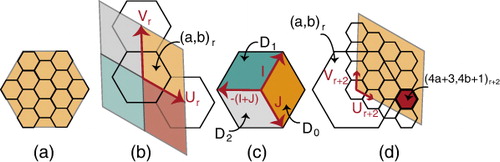
Table 4. (i,j) is covered by D_k if it falls in the ranges below.

Diamonds	Ranges
D0	0 ≤ i ≤ 1
	0 ≤ j ≤ 1
D1	0 ≤ −i ≤ 1
	0 ≤ −i ≤ 1
D2	0 ≤ −j ≤ 1
	−1 ≤ i + j ≤ 0

Using diamonds, we are not only able to provide a simple hierarchical coverage to traverse through the resolutions using the congruent hierarchy, but we are also able to exactly determine the fine hexagons that are covered by a coarse hexagon using incongruent hierarchy. However, fractal coverages are unable to efficiently support this operation as they do not provide exact fine hexagons covered by a coarse hexagons. As a result, our diamond-based hierarchy outperforms fractal coverages in both data analysis queries and hierarchical traversal.

6. Comparison and results

In this section, we discuss the usability of our indexing method and compare it to a 1D indexing proposed in Vince and Zheng (2009) and developed by PYXIS Innovation (2014). PYXIS indexing is similar to the set of 1D indexing methods proposed in Sahr, White, and Kimerling (2003), Middleton and Sivaswamy (2005), and Gibson and Lucas (1982); therefore, our comparison and claims are still valid for these 1D indexings. We describe PYXIS indexing and then demonstrate some of the results of our method implemented in PYXIS software that uses spherical icosahedron and 1-to-3 c-refinement. We also provide results on other refinements and polyhedrons.

6.1. PYXIS indexing

PYXIS indexing is designed for 1-to-3 c-refinement of an icosahedron (Vince and Zheng 2009). The initial application of such a refinement results in a truncated icosahedron. In this indexing scheme, each face of the truncated icosahedron is indexed by a number or letter. Afterward, cells are categorized into two types A and B, generating different fractal shapes throughout the resolutions that perfectly fit together and cover the entire surface of the spherical icosahedron. Each type B cell is surrounded by six type A cells.

The fine cell sharing a centroid with a coarse cell is called the centroid child. Other fine cells, whose centroids are aligned with the vertices of a coarse cell, are called vertex children. A type B cell with index b has a centroid child with index and six other vertex children with indices based on their direction to b. Only the centroid child of a type A cell a inherits its index from a receiving index . Centroid children and vertex children are considered to be of type B and A, respectively, at the next resolution, and a similar process of indexing is applied to these finer cells. This way, the set of children of a cell at fine resolutions features a fractal shape boundary (see Figure 13). Consequently, a cell at resolution r has index in which and m is an arbitrary initial letter or number representing the parent cell at the coarsest level.

Figure 13. (a) Type A cells (orange) surround a type B cell (black) with index α. (b) The children of cells illustrated in (a), (c), and (d). The children of type A and B cells, respectively, at five successive resolutions. Notice the fractal boundary developing at the finer resolutions.

6.2. Operation comparison

In this section, we compare the performance of our indexing to the important geospatial operations of neighborhood finding, hierarchical traversal and conversion to Cartesian coordinate systems.

6.2.1. Neighborhood finding

Finding the neighbors of a cell is one of the fundamental queries within a Digital Earth framework. Our indexing method handles neighborhood finding operations simply by adding neighborhood vectors to the index of a hexagon (Figure 14(a)).

Figure 14. (a) Neighborhood vectors for hexagons. (b) Hexagons assigned to diamond d_i. (c) Indexing the edges of a diamond. (d) We wish to find the neighbors of red hexagon (2,1)₀. The blue hexagons are obtained by adding neighborhood vectors to (2,1)₀ (the red hexagon). These blue hexagons lie outside diamond d₁. Hence, they are each mapped to a valid green hexagon in diamond d₂.

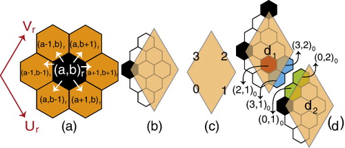
Some cells located at the boundary edges of the initial diamonds of an unfolded polyhedron may have neighbors belonging to another diamond. A boundary edge of diamond d_i is denoted by (see Figure 14(c)). To find the index of such cells, we use a mapping from a boundary edge of a diamond d_i to its adjacent diamond d_k in the polyhedron along the same edge . These mappings are listed in Table 5 (right). Given the mapping and constraints for each edge (refer to Table 5 (left)), the index of a cell on a boundary edge is mapped to an index in the coordinate system of . For example, if , index is mapped to . Note that Max is a constant for any refinement and resolution referring to the maximum index. For example, for 1-to-4 refinement . Figure 14 illustrates this scenario for an icosahedron when Max = 3, i = 1, and k = 2.

Table 5. Left: constraints on the indices of edges. j is variable and Max is a constant. Right: each edge of diamond d_i denoted by d_i(t) is connected to an edge d_j(v).

Edge	Constraint	Polyhedron	di(0)	di(1)	di(2)	di(3)
0	(j, 0)	Icosahedron	di−1(2)	di+1(3)	di+2(3)	di−2(3)
1	(Max, j)		di−2(1)	di+2(0)	di+2(0)	di−1(1)
2	(j, Max)	Octahedron	di−1(1)	di+1(0)	di+1(3)	di−1(3)
3	(0, j)	Tetrahedron	di+1(0)	di+1(3)	di+1(2)	di+1(1)

Note: Subscript addition for the d_i is modulo n, where n is the number of diamonds in the polyhedron. First/second rows of the icosahedron is for odd/even i.

Neighborhood finding under PYXIS indexing is handled using a large look-up table (19 × 12 entries) through an algorithm with time complexity of O(r) for resolution r (Vince and Zheng 2009). In our proposed indexing method, the neighbors of a hexagon are determined in constant time (O(1)) using simple neighborhood vectors. This difference in time complexity, which is independent of the implementation, makes our indexing superior to PYXIS indexing in operations that require neighborhood finding.

6.2.2. Hierarchical traversal

Traversing from one resolution to another is an important operation for analyzing and visualizing data present at different resolutions. In PYXIS indexing to traverse through resolutions only a digit is appended or dropped from the index in case of increasing or decreasing the resolution. This operation is performed in O(1) in PYXIS indexing. In our proposed indexing, we can also perform with the same efficiency by multiplying R or (scalar) to the index of a given cell.

6.2.3. Converting to Cartesian coordinates

Many available datasets are based on traditional Cartesian coordinates or coordinates that are simply converted to Cartesian coordinates such as lat–long spherical coordinate systems. As a result, finding Cartesian coordinates of a given cell (i.e. its centroid) is an important operation. In PYXIS indexing, each in the index is compatible with a vector in Cartesian coordinates. Then the coordinates of a given cell are found as a combination of all vectors corresponding to which performs in O(r). In our proposed method, the coordinates of a given cell at resolution r is found by multiplying T_r into its index that can be done in O(1).

6.3. Rendering

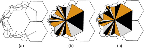
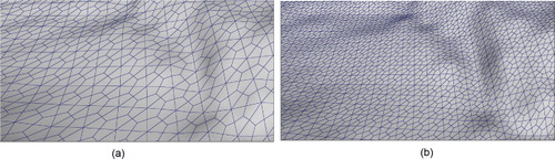
For storing, analyzing, and managing data in Digital Earth frameworks, hexagons are a good choice. However, to efficiently render hexagonal cells on the Earth's surface, they must be triangulated. Fractal-based (PYXIS) hierarchies are difficult to triangulate and due to the high-detail fractal boundary shape tend to result in poor triangulations. Guenette and Stewart (2008) suggest a method for an improved triangulation of fractal coverage. Although it is much better than a brute force triangulation of the hierarchical coverage (Figure 15(b)), poor skinny triangles and high-valence vertices still exist in the final result (Figure 15(c)).

Figure 15. (a) An adaptive fractal coverage. (b) Poor triangulation of the coverage illustrated in (a). (c) Improved triangulation using the proposed method in Guenette and Stewart (2008).

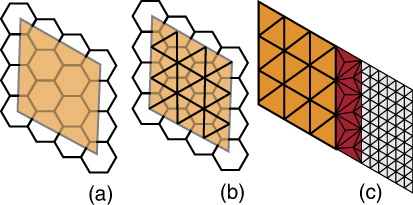
Diamond-based hierarchy, triangulating hexagons is easy and efficient with the resulting triangulated mesh being GPU-friendly (Pharr and Fernando 2005) (see Appendix B). To triangulate a diamond covering a set of cells, we create the dual mesh formed by connecting the centroids of the hexagons (Figure 16). For level-of-detail purposes, two diamonds might be at different resolutions. We connect these diamonds to each other via a method similar to the adaptive refinement of subdivision (Kobbelt 2000). We show how to connect two diamonds resulting from 1-to-3 c-refinement in Figure 16. Other refinements are handled similarly.

Figure 16. (a) A set of hexagons covered by a diamond. (b) Triangulation of a diamond. (c) Two diamonds at two different resolutions. Red portion shows the transition between two resolutions to avoid cracks.

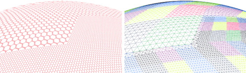
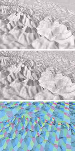
To illustrate diamond coverage, its correspondence to hexagons are visualized in Figures 17–20. Triangulation of a portion of the globe at two successive resolutions of 1-to-4 c-refinement and its triangulation are illustrated in Figure 17. An octahedral Digital Earth resulting from a 1-to-7 refinement is illustrated in Figure 18. Figure 19 illustrates a portion of the globe (icosahedral with 1-to-3 refinement) in a close up view. The transition between diamonds at two different resolutions is noticeable. In Figure 20, we visualize the elevation data corresponding to hexagonal cells.

Figure 17. Triangulation of a hexagonal terrain at two successive resolution of 1-to-4 refinement.

Figure 18. (a) Hexagonal faces resulting from 1-to-7 refinement on an octahedron. Each initial diamond is rendered in a different color. (b), (c) Spherical octahedron with hexagonal cells. (d) Textured spherical polyhedron.

Figure 19. Hexagonal cells (left) and their corresponding triangulations (right).

Figure 20. A portion of the Earth's surface having elevation data. Top: the hexagonal cells with associated elevation data. Middle: the parents of the hexagonal cells in the top figure at three successive resolutions. Bottom: the triangulation of the diamonds corresponding to the cells illustrated in the top figure. Image is taken from PYXIS Innovation (2014).

7. Conclusion

In this paper, we present a multiresolution indexing method for hexagonal cells. This indexing works with hexagonal lattices formed on unfolded polyhedra. By providing aligned coordinate systems, we obtain constant-time hierarchical and neighborhood finding operations, as well as conversion to Cartesian coordinate systems. We demonstrate two diamond-based hierarchies simplifying the coverage problem for the boundaries of polyhedra. Such a diamond-based hierarchy is very useful for triangulating hexagonal cells to support efficient rendering. We show how this method works efficiently by providing several example results.

Acknowledgments

We are grateful to Idan Shatz for insightful discussions. Without his valuable inputs, this research was impossible. We also thank Troy Alderson for editorial comments.

Funding

This research was supported in part by PYXIS Innovation, the National Science and Engineering Research Council of Canada, and GRAND Net-work of Centre of Excellence of Canada.

Additional information

Funding

Funding: This research was supported in part by PYXIS Innovation, the National Science and Engineering Research Council of Canada, and GRAND Net-work of Centre of Excellence of Canada.

Appendix A: Origin of translated 1-to-3 refinement

As discussed earlier, is chosen for the origin of resolution r + 1 when r is even, and for odd r. Thus, for , we have the origin at . Since and similarly , we have . From the sum of the first n terms of this geometric series, the locus of the origin is . This is one possibility for determining the origin of the subsequent resolutions. Alternative origins may lead to different but closed form formulae.

Appendix B: GPU rendering of triangulated diamonds

Figure B1. (a) A triangulated diamond with triangle strips in different colors. (b) The indices of the vertices of a diamond for array I = (1, 5, 2, 6, 3, 7, 4, 8, 8, 5, 5, 9, 6, 20, …). Degenerate triangles form at (4, 8, 8), (8, 8, 5), (8, 5, 5), and (5, 5, 9).

Given a triangulated diamond, we can efficiently render it using built-in OpenGL functions such as glDrawElements() to simultaneously pass an array of vertices to the GPU (Munshi, Ginsburg, and Shreiner 2008, Chapter 7). To do so, we make two arrays V and I. V stores the 3D locations of the vertices while I refers to the indices of the vertices in V. The indices of I are sequentially ordered to make rows of triangle-strips in a diamond. Note that a vertex with 2D index has index in array V if the diamond has vertices. At the last vertex of each row, we form degenerate triangles to link up the rows. These degenerate triangles are not rendered and handled by the GPU. V and I are then passed to glDrawElements() and rendered in mode. Figure B1 illustrates an example for a diamond and array I.

References

- Alborzi, H., and H. Samet. 2000. “Augmenting Sand with a Spherical Data Model.” First International Conference on Discrete Global Grids, Santa Barbara, CA, March 26–28.
- Ben, J., X. Tong, and R. Chen. 2010. “A Spatial Indexing Method for the Hexagon Discrete Global Grid System.” 2010 18th International Conference on Geoinformatics, 1–5, Las Vegas, Nevada, June 18–20.
- Burt, P. J. 1980. “Tree and Pyramid Structures for Coding Hexagonally Sampled Binary Images.” Computer Graphics and Image Processing 14: 271–280. doi:10.1016/0146-664X(80)90056-8.
- Cashman, T. J. 2012. “Beyond Catmull-clark? A Survey of Advances in Subdivision Surface Methods.” Computer Graphics Forum 31 (1): 42–61. doi:10.1111/j.1467-8659.2011.02083.x.
- Chen, J., X. Zhao, and Z. Li. 2004. “An Algorithm for the Generation of Voronoi Diagrams on the Sphere Based on QTM.” Photogrammetric Engineering and Remote Sensing 69 (1): 79–89. doi:10.14358/PERS.69.1.79.
- Claes, J., K. Beets, and F. Van Reeth. 2002. “A Corner-cutting Scheme for Hexagonal Subdivision Surfaces.” Proceedings of the Shape Modeling International 2002 (SMI'02), Washington, DC, IEEE Computer Society, 13–20, Banff, Alberta, Canada, May 17–22.
- Cozzi, P., and K. Ring. 2011. 3D Engine Design for Virtual Globes. 1st ed. Boca Raton: CRC Press.
- Dutton, G. 1999. A Hierarchical Coordinate System for Geoprocessing and Cartography. Lecture Notes in Earth Sciences Series. Berlin: Springer Verlag.
- Faust, N., W. Ribarsky, T. Jiang, and T. Wasilewski. 2000. “Real-time Global Data Model for the.” Proceedings of the International Conference on Discrete Global Grid, Santa Barbara, CA, March.
- Fekete, G., and L. A. Treinish. 1990. Sphere Quadtrees: A New Data Structure to Support the Visualization of Spherically Distributed Data, 242–253, Santa Barbara, CA, February.
- Gibson, L., and D. Lucas. 1982. “Spatial Data Processing Using Generalized Balanced Ternary.” Proceedings of the IEEE Computer Society on Pattern Recognition and Image Processing, 566–572, Las Vegas, June 14–17.
- Goodchild, M. F. 2000. “Discrete Global Grids for Digital Earth.” Proceedings of 1st International Conference on Discrete Global Grids, Santa Barbara, CA, March 26–28.
- Guenette, M., and A. J. Stewart. 2008. “Triangulation of Hierarchical Hexagon Meshes.” Proceedings of the 2008 ACM Symposium on Solid and Physical Modeling, SPM'08, 307–313, New York, June 2–4.
- He, X., and W. Jia. 2005. “Hexagonal Structure for Intelligent Vision.” First International Conference of Information and Communication Technologies, ICIT 2005, 52–64, Karachi, Pakistan, August 27–28.
- Ivrissimtzis, I. P., N. A. Dodgson, and M. A. Sabin. 2004. “A Generative Classification of Mesh Refinement Rules with Lattice Transformations.” Computer Aided Geometric Design 21 (1): 99–109. doi:10.1016/j.cagd.2003.08.001.
- Kamgar-Parsi, B., B. Kamgar-Parsi, and W. A. Sander. 1989. “Quantization Error in Spatial Sampling: Comparison between Square and Hexagonal Pixels.” Proceedings CVPR'89, IEEE Computer Society Conference on Computer Vision and Pattern Recognition, 604–611, San Diego, CA, June 4–8.
- Kobbelt, L. 2000. “ ! subdivision.” SIGGRAPH'00: Proceedings of the 27th Annual Conference on Computer Graphics and Interactive Techniques, 103–112, New Orleans, July 25–27.
- Mahdavi-Amiri, A., F. Bhojani, and F. Samavati. 2013. “One-to-two Digital Earth.” ISVC 8034 (2): 681–692.
- Middleton, L., and J. Sivaswamy. 2005. Hexagonal Image Processing: A Practical Approach (Advances in Pattern Recognition). Secaucus, NJ: Springer-Verlag New York.
- Munshi, A., D. Ginsburg, and D. Shreiner. 2008. OpenGL ES 2.0 Programming Guide. 1st ed. Reading, MA: Addison-Wesley Professional.
- Peterson, P. 2006. Close-packed, Uniformly Adjacent, Multiresolutional, Overlapping Spatial Data Ordering. Filed on August 1, 2003, Canadian Patent, CA 2436312, EP Patent App. EP20,040,761,671.
- Pharr, M., and R. Fernando. 2005. GPU Gems 2: Programming Techniques for High-performance Graphics and General-purpose Computation. Reading, MA: Addison-Wesley Professional.
- PYXIS Innovation. 2014. “Pyxis Indexing.” Accessed February. http://www.pyxisinnovation.com.
- Sadourny, R., A. K. I. O. Arakawa, and Y. A. L. E. Mintz. 1968. “Integration of the Nondivergent Barotropic Vorticity Equation with an Icosahedral-hexagonal Grid for the Sphere.” Monthly Weather Review 96 (6): 351–356. doi:10.1175/1520-0493(1968)096%3C0351:IOTNBV%3E2.0.CO;2.
- Sahr, K. 2008. “Location Coding on Icosahedral Aperture 3 Hexagon Discrete Global Grids.” Computers, Environment and Urban Systems 32 (3): 174–187. doi:10.1016/j.compenvurbsys.2007.11.005.
- Sahr, K. 2011. “Hexagonal Discrete Global Grid Systems for Geospatial Computing.” Archives of Photogrammetry, Cartography and Remote Sensing 22: 363–376.
- Sahr, K., D. White, and A. J. Kimerling. 2003. “Geodesic Discrete Global Grid Systems.” Cartography and Geographic Information Science 30 (2): 121–134. doi:10.1559/152304003100011090.
- Samet, H. 2005. Foundations of Multidimensional and Metric Data Structures (The Morgan Kaufmann Series in Computer Graphics and Geometric Modeling). San Francisco, CA: Morgan Kaufmann.
- Snyder, J. P. 1992. “An Equal Area Map Projection for Polyhedral Globes.” Cartographica 29: 10–21. doi:10.3138/27H7-8K88-4882-1752.
- Snyder, W. E., H. Qi, and W. Sander. 1999. “A Coordinate System for Hexagonal Pixels.” The International Society for Optical Engineering 3661: 716–727.
- Thuburn, J. 1997. “A PV-based Shallow-water Model on a Hexagonal-icosahedral Grid.” Monthly Weather Review 125 (9): 2328–2347. doi:10.1175/1520-0493(1997)125%3C2328:APBSWM%3E2.0.CO;2.
- Tobler, W., and Z.-t. Chen 1986. “A Quadtree for Global Information Storage.” Geographical Analysis 18 (4): 360–371. doi:10.1111/j.1538-4632.1986.tb00108.x.
- Tong, X., J. Ben, Y. Wang, Y. Zhang, and T. Pei. 2013. “Efficient Encoding and Spatial Operation Scheme for Aperture 4 Hexagonal Discrete Global Grid System.” International Journal of Geographical Information Science 27 (5): 898–921. doi:10.1080/13658816.2012.725474.
- Vince, A. 2006. “Indexing the Aperture 3 Hexagonal Discrete Global Grid.” Journal of Visual Communication and Image Representation 17 (6): 1227–1236. doi:10.1016/j.jvcir.2006.04.003.
- Vince, A., and X. Zheng. 2009. “Arithmetic and Fourier Transform for the PYXIS Multi-resolution Digital Earth Model.” International Journal of Digital Earth 2 (1): 59–79. doi:10.1080/17538940802657694.
- Wartell, Z., E. Kang, T. Wasilewski, W. Ribarsky, and N. Faust. 2003. “Rendering Vector Data over Global, Multi-resolution 3D Terrain.” Proceedings of the symposium on Data Visualisation 2003, VISSYM'03, 213–222, Grenoble, France, May 26–28.
- White, D. 2000. “Global Grids from Recursive Diamond Subdivisions of the Surface of an Octahedron or Icosahedron.” Environmental Monitoring and Assessment 64 (1): 93–103. doi:10.1023/A:1006407023786.
- White, D., J. A. Kimerling, and S. W. Overton. 1992. “Cartographic and Geometric Components of a Global Sampling Design for Environmental Monitoring.” Cartography and Geographic Information Science 19 (1): 5–22. doi:10.1559/152304092783786636.
- Wickman, F. E., E. Elvers, and K. Edvarson. 1974. “A System of Domains for Global Sampling Problems.” Geografiska Annaler. Series A, Physical Geography 56 (3/4): 201–212. doi:10.2307/520707.