Understanding the potential relationship between the socio-economic variables and contributions to OpenStreetMap

Abstract

OpenStreetMap (OSM) has seen an exponential increase in the last few years and large volumes of geodata have been received from volunteered individuals. The collected geodata are heterogeneous in terms of different dimensions such as spatial patterns of contributions, quality, patterns of contributing individuals, and type of contributions. Because contributors’ personal information is anonymously stored by the OSM administrators, alternative methods are needed to investigate the role of contributors’ characteristics on their mapping behavior. This study is intended to explore the potential socio-economic characteristics of contributors in highly contributed areas to have better insights about the latent patterns of involved individuals in a highly dynamic state of the most active country in OSM, Germany. A logistic regression model (LRM) is applied to discover the potential correlations between dependent and independent variables. The findings explain that the areas with high population density, middle level of education, high income, high rate of overnight stays, high number of foreigners, and residents aged from 18 to 69 are more likely to be involved in OSM. Furthermore, the degree of dynamism in OSM is a function of proximity to built-up areas. Finally, concluding remarks concerning the independent variables and model sensitivity are presented.

Keywords:

• OpenStreetMap
• spatial analysis
• collaborative mapping
• logistic regression analysis
• social science

1. Introduction

Since the widespread development and dissemination of volunteered geographic information (VGI; Goodchild 2007) projects, OpenStreetMap (OSM) has proven itself as a catalyst for an open mapping revolution (Chilton 2011), because it has offered a wide range of applications and extensions for diverse purposes and that is why it has become the most exemplary instance of VGI projects (Lin 2011). There are of course further reasons for that such as – the genealogy of every object in OSM can be tracked in order to see how an object has developed over time. The combination of mapped objects, the documentation, user diaries, blogs, mailing lists, forums, and wiki pages are also additional valuable sources of information that help to mine further information about geodata from OSM (Perkins 2014). The contribution of OSM in supporting digital earth applications as outlined by Craglia, de Bie et al. (2012) and Craglia, Ostermann et al. (2012) is discussed in details by Mooney and Corcoran (2013b). They believe that the increasing and steady success of OSM in attracting mappers and in capturing diverse types of objects at finer resolutions than mapping agencies’ products will certainly present a dynamic digitalized ecosystem toward developing digital earth applications. So far, several applications based on OSM have been developed such as routing (Bakillah, Lauer et al. 2014), indoor mapping (Goetz 2012), population mapping based on points-of-interest (Bakillah, Liang et al. 2014), land use mapping (Jokar Arsanjani, Helbich, Bakillah et al. 2013; Hagenauer and Helbich 2012), and deriving buildings footprints (Fan et al. 2014) or digital elevation models (Klonner et al. 2014), among other examples.

Lately, there has been an exponentially increasing interest in getting involved in contributing in OSM as noted by Neis and Zielstra (2014) and Jokar Arsanjani et al. (2014). The degree of involvement and receipt of contributions from across the world has varied across space and time, coming largely from the developed countries, more particularly from Germany, Austria, Great Britain, France, and the USA, if we disregard the bulk imports from official datasets (Neis, Zielstra, and Zipf 2013). There is, however, no substantial information about the emergence and evolution of OSM in developing countries to see how differently people welcome OSM to share their information.

It is certainly crucial to understand what is behind the uneven distribution of contributions to OSM in order to gain profound insights about the motivations that drive contributors, as studied by Haklay and Budhathoki (2010). Doing so would enable us to evaluate the trustworthiness, accuracy, representativeness, and uncertainty of contributions and whether it is linked to the socio-economic, physical, and behavioral characteristics of the contributors. The mapping manner and the spatial distribution of them may be related to various social and economic characteristics of mappers (Budhathoki 2010).

The patterns of individuals in the cyberspace have been vastly investigated either through online and offline surveying and questionnaires or through statistical analysis (Bimber 2000; Shaw and Gant 2002; Ono and Zavodny 2003; Calvert et al. 2005; Rutten et al. 2012; White and Selwyn 2013). They concluded that gender, age, race, education, level of income, and other socio-economic variables highly impact the patterns of Internet users across the globe and a fluctuating correlation between them can be explored depending on time and space.

Collaborative mapping is related to motivational factors as noted by Coleman et al. (2009) and Budhathoki, Haklay, and Nedovic-Budic (2010), which is also dependent on individuals’ actions. Similar investigations to those mentioned earlier for the Internet users for discovering the relationships between the OSM users and their mapping were conducted in the early days of OSM. For instance, Perkins and Dodge (2008) revealed that OSM users at the time of involvement in OSM are strongly gendered, that is, almost all of the OSM activists are male with particular male stereotypic behaviors. They also concluded that undoubtedly there are cultural differences in participation across nations, although not statistically proven. Moreover, Haklay and Budhathoki (2010) considered a sample (n = 426) of contributors to study the social demographics of participation and they realized that it has a very unequal pattern so that 96% of sampled OSM mappers were male, 78% had taken university education, and 86% were aged 20–50. The sample of participants were mainly young educated men involved in technology-related jobs, and 51% even had some experience in GIScience. Mashhadi, Giovanni, and Capra (2013) investigated which contextual factors correlate with OSM coverage in urban environments and found that in addition to population density, other potential socio-economic factors also play an important role in the quality of the OSM coverage.

Whereas using online questionnaires is time consuming and labor intensive and also the investigation relies on a small number of participants, in the case of OSM, we faced a different type of problem. Because the OSM users remain anonymous and their personal profiles and Internet Protocol (IP) tracks is not accessible for statistical analysis, we need to uncover the spatial and temporal patterns of their geospatial contributions and compare it with their demographic and economic patterns, as provided, for example, through official data sources. As OSM provides us with each individual's mapping activity and the history of their activities, we can track the patterns of their activities in OSM and accordingly investigate the potential socio-economic driving factors of their mapping behavior. This approach would be a practical way to indicate their characteristics. Several studies dealing mainly with the contributors-centric perspectives of OSM have been conducted, such as analysis of interaction and co-editing patterns amongst OSM contributors by Mooney and Corcoran (2013a), the emergence and evolution of OSM by Jokar Arsanjani et al. (2014), and the comparison of the OSM contributions across selected cities in regard with the impact of their national gross domestic product (GDPs) (Neis, Zielstra, and Zipf 2013), among others. However, no specific study has statistically (and not based on surveying) assessed the possible relationships between the location of contributions and the characteristics of local residents, because the mapped objects are assumedly implicative of local residents’ interactions with environment.

The main objective of this study is to use the contributions to OSM in order to explore the spatial patterns of the contributions as well as the driving factors that could possibly characterize the underlying relationships between the contributions and the socio-economic characteristics of local inhabitants. This study applies an exploratory analysis of a subset of OSM contributors and their contributions with the focus on highly contributed areas. It is presumed that the location of contributions indicates the socio-economic patterns of their contributors.

The remainder of the study is structured as follows. Section 2 describes the materials used in this study. Section 3 presents the methods applied. Section 4 presents the results followed by a discussion on the achieved results. Finally, Section 5 concludes with a discussion of implications and future research directions.

2. Materials

2.1. Study area

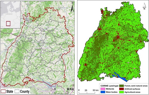
In this study, the Baden-Württemberg state of Germany was selected as shown in Figure 1. The reasons for choosing this study area are twofold: first, Germany as a whole has been known as a representative country in OSM and the selected area has been a dynamic area in receiving a large amount of contributions; second, the selected area consists of several counties characterized by dissimilar socio-economic and physical variables. The physical patterns extracted from CORINE land cover dataset are shown in Figure 1.

Figure 1. The geographical extent of Baden-Württemberg state of Germany as the study site (left), CORINE land cover map of the study area (right).

2.2. Data

The dataset used in this investigation are the OSM nodes extracted from the OSM-dump file in 17 July 2013 that represents every node that has been contributed to OSM. In total, there are 20,435,026 nodes collected from 10,032 users over the Baden-Württemberg state of Germany.

In order to investigate the relationships between the contributions and socio-economic and physical characteristics in the study area, the socio-economic data at county level (Kreise) were collected, because (1) this is the finest level that is freely available to public, (2) it is presumed that local residents of each county are more likely to map their states. The socio-economic data were freely accessible through the federal statistics center of Germany (www.destatis.de). Several attributional variables were linked to the state's counties and accordingly spatialized. Proximity to built-up areas is also considered in this study as a physical characteristic. CORINE land cover dataset provided the footprints of built-up areas (Figure 1). Table 1 describes the utilized variables and their dates of collection.

To create a compatible set of variables, all variables were normalized by the total number of people in each county and then ranged in 0–255.

Table 1. Dependent and independent variables used in the logistic regression model.

Variables	Acronym	Denotation	Date of collection	Data range
Dependent	Hot spots	Highly contributed areas	31 December 2012	–
Independent	FP	Percent of foreigners	2011	5–24%
	In	Annual income	2009	17,613–31,020 €/year
	OS	Overnight stays	2011	205,212–16,032,421
	Tx	Paid tax on the income	2007	288,941–2,371,225 €/year
	PD	Population density	2011	102–2958.2 persons/km^2
	SW	Social welfare	2004	1384–23,517
	UR	Unemployment rate	2012	2.6–7.7%
	BHS	People with education level below high school	2011	12.2–25.5%
	PT	People with practical training	2011	49.3–66.7%
	EP	Educated people	2011	4.9–22.3%
	AG1	Age group 1: below 18 years old	2011	13–19%
	AG2	Age group 2: 18–50 years old	2011	38–53%
	AG3	Age group 3: 50–70 years old	2011	21–26%
	AG4	Age group 4: >70 years old	2011	13–22%
	DtB	Distance to built-up areas	2006	–

3. Methods

Contributors are expected to map the places that they have ever been to or visited or at least to which they are somehow connected (Haklay and Budhathoki 2010). However, it has not been practically proven that people map places of their interest. In this section, we attempt to understand the characteristics of highly contributed areas by studying the relationships between their spatial occurrences and the socio-economic characteristics of individuals.

Since the study area has received a large number of contributions, which are spread over the study area, the hot spots from the whole dataset were filtered. To do so, the contributed nodes were abstracted into a cellular grid consists of cells with 1 km*1 km size resulting in 36,900 cells. Each cell of the grid contains the number of contained nodes as well as osmversion within each cell. Thereafter, in order to ascertain the cells with high density of nodes, a hot spot analysis based on the Getis-ord Gi* method is applied to detect hot spots in which high number of contributions are received by a larger number of users. The Getis-ord Gi* statistic identifies clusters with values higher in magnitude than we expect to find by chance (Anselin 1995). It is presumed that hot spots are likely to represent some particular characteristics of individuals and the physical environment such as age group, educational attainment, household income, population density, tourists, unemployment, nationality, paid taxes, proximity to developed areas, and social welfare.

Considering the ecological correlations (Robinson 1950) between location of high contributions and the socio-economic and physical characteristics of users suggests that states with specific characteristics of individuals are better mapped than others and hence a correlation between these areas and local residents and environment can be explored. Although the connection of OSM contributions, contributors, and their activities with the local residents is likely to be complex, this investigation attempts to assess the latent and potential relationships between the characteristics of users and environment and contributions.

Next, a binomial logistic regression model (LRM) is conducted using two main variables associated with OSM mapping (1) the dependent variable, (2) independent variables. A binary file identifying the location of hot spots was assigned as the dependent variable.

3.1. Logistic regression model

Regression has been widely applied in similar cases for testing the effects and the importance of the effects in a simple and straightforward manner (Holland 1986; Wang et al. 2013; Jokar Arsanjani, Helbich, Kainz et al. 2013). Logistic regression is considered as a suitable regression tool in this case, because the binary dependent variable is controlled by a number of variables (Cheng and Masser 2003; López and Sierra 2010). For this study as a pioneering investigation focused on OSM, a classical regression framework is selected to identify the possible impacts of the proposed independent variables and to see how they are connected with the highly mapped areas. This enables us to estimate spatially explicit binary LRM of the mapping process (Mertens et al. 2004). The LRM is formed as follows:

where y is the probability of high contribution, ß ₀ is the intercept, ß is a vector of estimated parameters, x is a vector of driving factors, and ε is a randomly distributed residual error (Lin 2011).

Computed regression coefficients indicate the direction (±) and intensity of the influence of the independent variables on the probability of high contributions. They are also used to compare the relative effects of each independent variable on the intensity of mapping (e.g. Long and Freese 2006). In theory, dependent and explanatory variables might be spatially auto-correlated, which might bias the results of the LRM (Crk et al. 2009; Luo and Wei 2009). Therefore, in order to avoid this conflict in the computational process, a stratified random data sampling approach is applied, which integrates systematic and random sampling (Cheng and Masser 2003; Crk et al. 2009).

3.2. Dependent variable

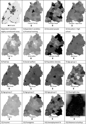
Highly contributed areas are considered as the dependent variable. ‘One’ pixels represent all pixels that correspond to hot spots of contributions, while ‘zero’ pixels represent all pixels where the number of contribution was not high. As mentioned earlier, the Getis-ord Gi* function was applied to filter these areas by the end of 2012 (see Figure 3). The independent and dependent variables are shown in Figure 2.

Figure 2. Independent and dependent variables in the LRM.

3.3. Selecting the independent variables

Socio-economic development is one of the most important driving factors of individuals’ contribution. Additionally, the physical characteristics of undertaken areas play an important role in receiving contributions. The set of independent variables incorporates a variety of socio-economic variables. A few researches dealing with statistical analysis of the characteristics of contributors in OSM have been reported such as Neis, Zielstra, and Zipf (2013) which noted that the amount of contributions in OSM at a global level for selected countries depends on the population and GDP of each country. Furthermore, Li, Goodchild, and Xu (2013) studied the possible relationships between the socio-economic variables and the density of tweets and Flickr photos in the USA. Therefore, we decided to include the review of relevant literatures in other disciplines such as urban expansion (e.g. Avelar et al. 2009; Drummond et al. 2012; Jokar Arsanjani, Helbich, Kainz et al. 2013; Li, Zhou, and Ouyang 2013), number of Internet users (e.g. Brouwer et al. 2010; Hernández, Jiménez, and José Martín 2011; Schneider, van Osch, and H. de Vries 2012), disease disorder (Généreux, Bruneau, and Daniel 2010; Williams et al. 2011), and farming development (Müller et al. 2011) in order to gain insights into the economic and social context of contribution. Descriptive information of the mentioned variables in Table 1 is depicted as follows.

3.3.1. Social indicators

Age group

It is presumed that age plays an important role in mapping OSM, as people of a certain age may have limited mapping skills. For instance, the youngest category of people (below 18 years old) may have never received the required knowledge and training to contribute. Additionally, the oldest category of inhabitants (above 70 years old) may not, generally, be familiar enough with Internet technologies to contribute to OSM. Hence, the two middle categories (18–50 and 50–69 years old) are subject to mapping. This variable was imported into the model containing four categories of residents as shown in Table 1. The spatial distribution of age groups shows that the counties with larger urban areas contain a larger portion of young population than counties with rural population. On the contrary, the old population is located in the states with rural areas and mid-size towns. Similarly, the population density as a whole is higher in large urban areas. Population density is also considered in the model as the more people live within a state, the more potential mappers might sign up and map their surroundings.

Education

The degree of education is also likely to influence the mapping behavior, as educated people may be more familiar with Internet technologies. Presumably, less educated people may lack the skills to contribute while educated people may be more interested in mapping. Three categories are designed for this variable: education below high school, people with practical training, and people with above high school education. Typically, the spatial distribution of education is also in favor of larger urban areas so that Stuttgart, Freiburg, Karlsruhe, Mannheim, and Heidelberg contain more educated and practically trained people (Figure 2).

Foreigners

As a considerable amount of people are foreigners and have dissimilar characteristics, the percentage of foreign people is considered as an independent variable. Since Germany has been the best mapped country in OSM and also is the target of immigration for other nationals, therefore considering whether foreign people positively or negatively impact the mapping seems to be important. The foreign population is mainly located in larger urban areas as typically, the job market situation and demand in cities is higher than in rural areas.

3.3.2. Economic indicators

Average annual income of people

Paid income tax, social welfare, unemployment rate, and reported overnight stays are also other economic variables that might have an impact on the mapping. The number of reported overnight stays per area is considered, because it is presumed that the more people come to a state and the more the state is visited, the more potential mappers know the area and therefore it may be mapped by more people than its own residents. The spatial distribution of these variables is also in favor of urban areas so that more taxes are paid, more social welfare from the state government is paid, the rate of unemployment is higher, and more visitors arrive and stay overnight.

3.3.3. Physical characteristics

Proximity to built-up areas is considered as a potential driving factor in receiving massive contributions from individuals. It is presumed that developed areas and their surroundings are better mapped, because first, these areas contain more people and therefore are mapped by the local residents, and second, in developed areas, more geographical objects exist that can be mapped.

3.4. Model configuration and validation

The correlation coefficients between the dependent and independent variables were computed by applying an LRM. A probability map representing the areas that are likely to be greatly mapped is calculated under the assumption that amount of contributions to OSM will expand linearly.

For the validation phase, a pseudo R ² value for each model was calculated for assessing the fit of LRM, whilst z-statistics was used to measure the significance of coefficients (Long and Freese 2006). Additionally, receiver operation characteristics (ROC: Pontius and Schneider 2001) was also assessed in order to evaluate the predictive accuracy of probability maps by calculating the area under the ROC curve (Wang et al. 2013). The ROC value confirms continuous calculated probabilities against binary observations. An ROC value of 0.5 indicates accuracy equal to a random model, while a value of 1 indicates perfect accuracy (Pontius and Schneider 2001; Verburg et al. 2004).

4. Results and discussion

4.1. Spatial distribution of contributions

Due to the large number of nodes, a grid network at grid size of 1000 m was designed in order to abstract the contributed nodes. The location of contributed nodes is plotted in Figure 3 and the CORINE land cover types are plotted in Figure 1. A visual analysis of high spots and nodes density confirm that the cells with high number of nodes and osmversion roughly delineate the artificial surfaces in which constructions are situated.

Figure 3. Hot spot analysis of nodes based on their quantity per cell (a) and kernel density analysis of nodes (b).

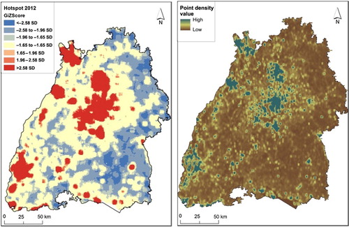
The total number of contributed nodes per cell and the mean osmversion per cell is used to identify hot spots. Getis-ord Gi* statistics was applied to identify hot spots, which contain the highest number of contributions that are edited the most. While red and blue cells (Figure 3a) identify hot and cold spots, respectively, yellow cells identify the regular cells that have received a fair amount of contributions. A kernel density analysis also confirms that the dense spots determine urban areas and their neighboring developments. In the study area, the biggest colony of hot spots is in the metropolitan area of Stuttgart, the capital and the largest city of Baden-Württemberg, while other hot spots identify Karlsruhe, Mannheim, Heidelberg, and Freiburg, which are the biggest cities of the state. On the contrary, cold spots identify either the areas where OSM mapping is not as active as other areas or these areas do not contain too many objects to be mapped.

4.2. Logistic regression analysis

LRM was effectively carried out to find the relationships between the highly contributed areas as the dependent variable and socio-economic and physical variables as independent variables. The response variable was a function of the selected variables at different effects and intensities. A set of LRMs with different numbers of independent variables was calibrated in the support of computed ROC value using a stratified random sampling within the mask of the 44 counties. The highest ROC value was achieved at 0.893 with a set of mentioned variables indicating a relatively high degree of spatial consistency between the model predictions and actual identified hot spots. This ROC value was the highest attained value, which verifies the selection of the best set of variables among the possible sets. The following equation depicts the achieved intercept and coefficient of each variable:

The model calibration phase resulted in a predicted probability surface map of future hot spots of contributions, as well as a residual map indicating the difference between the predicted and the observed probability for each set of variables. The social, economic, and physical variable factors together were significantly related to highly contributed regions in the study area. In the following note, the factors will be considered based on the coefficient values and their positive or negative influence of mapping behavior, respectively.

Distance to built-up areas and population density have positively and strongly caused intensive mapping. The impact of the former factor is reasonably explored as it has been previously confirmed by Neis, Zielstra, and Zipf (2013) and Jokar Arsanjani et al. (2014) that the urban areas have received relatively more contributions as more mappable objects in urban areas exist. In addition, more mappers are present within urban areas, which confirm the rationale of the latter factor.

Level of education has also a direct impact on the magnitude of received contributions as proven by the model: educated people and people who received practical training have also positively impacted the intensity of the mapping activity, while under high school educated people negatively affected the process. Based on the achieved coefficients, it is inferred that although uneducated people are unlikely to contribute, highly educated people contribute less than the middle category (i.e. practically trained individuals). This is the case in the study by Li, Goodchild, and Xu (2013) resulted in similar findings, as the people with bachelor's degrees were more likely to tweet or share their photos in Flickr.

The LRM reveals that the four age categories play different roles in OSM mapping as the youngest and oldest categories of age groups have negatively influenced the mapping process; contrarily to people within the age 18–69 who have contributed more to OSM. The coefficients relatively expose the same intensity of impact with the exception of the oldest group that impacts more than others.

The unemployment rate and social welfare capitation are related to lower contributions rates, suggesting that the more people are employed, the more intensely their surroundings are mapped. Social support from the state government seems to be also an influential driving factor with a negative impact on mapping activity so that the areas which receive more social benefits from government are very unlikely to be active in mapping. The remaining factors such as percentage of foreigners, income level, overnight stays, and tax have positive impacts on the mapping activity. In other words, if the amount of foreigners and overnight stays as a measure of tourism within an area increases, their surroundings seem to be more intensively mapped. This could be due to their interest in discovering their surroundings, regardless of their education, age category, etc. Similarly, more tax payers and high income people are more likely to contribute to OSM.

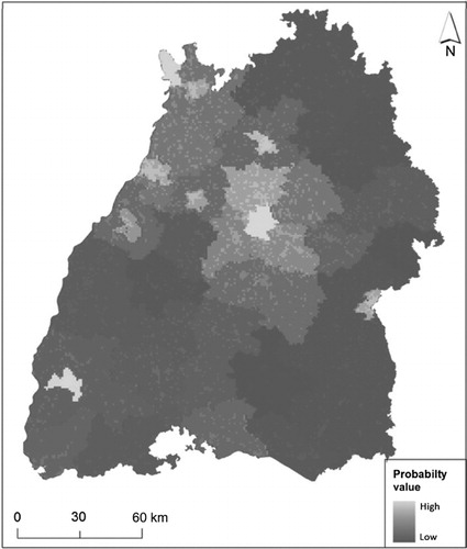
4.3. Probability map of future intensive mapping

A probability map specifies the likelihood of future intensive mapping across space and represents an important ingredient for future estimates of intense mapping and it can be also recycled for model validation (Verburg et al. 2006). This was carried out by calculating the area under ROC curve at 0.893, which confirms a relatively high degree of spatial consistency between the model predictions and actual identified hot spots. The generated probability map is shown in Figure 4. This must be mentioned that this map is based on the assumption that intense mapping activity will continue at the same rate as observed so far.

Figure 4. The probable spatial distribution of future contributions in OSM based on LRM.

5. Conclusions

The rapid evolution of collaborative mapping as seen in OSM as well as individuals’ rising interest and curiosity in contributing have motivated GIScience people, social scientists, cyberspace investigators, and others to dig more deeply into OSM and figure out how it performs and succeeds in attracting people. Due to the unequal and heterogeneous patterns of involved individuals, amount of data, quality of data, and types of data, more investigations on OSM contributions are needed. The successful story of OSM could be always depicted in order to develop other novel applications toward providing a digital earth involving social in digitalizing the existing objects and attributing them.

The relatively democratic mechanism of receiving, sharing, storing, and retrieving geodata in OSM has motivated the GI scientist and other related researchers to take OSM as a symbolic environment into account and lately they have begun to expend more efforts on it. Though, there are still many non-responded questions about the users as the central core of such a project to be answered. For instance, who are the OSM contributors? What are their characteristics from the whole body of the public? Data quality assurance efforts are also linked to the answers of these questions and once we know which people in the public are the main audience of OSM, then a human dimension of OSM can be better analyzed.

Despite the fact that collaborative mapping in OSM is very complex, this study cross compared the highly contributed areas within a cellular grid, which are distinguished based on application of a Getis-ord Gi* function, with the social, economic, and physical characteristics of the footprinted areas and local residents. A very dynamic area in OSM, Baden-Württemberg state of Germany, was selected for this investigation. Interestingly, the hot spots delineated the major cities of state of Baden-Württemberg. An LRM was applied considering the hot spots of contributions as the dependent variable, which its occurrences presumably depended on 15 independent variables, in order to understand the potential correlations between the hot spots and independent variables at a county level.

The findings resulted from the LRM reveal that the locations of highly contributed areas are positively dependent on the population density of the footprinted areas, level of education (in favor of middle class, i.e. not highly/barely educated), level of income, overnight stays as a measure of tourism, age groups (young to middle ages), and percentage of foreigners. Furthermore, proximity to built-up areas highly impact the degree of contributions so that the closest areas to developments are better mapped. On the contrary, residents with higher distributed social welfare and unemployment rate contribute less in OSM. The age groups of 1 and 4, which are the youngest and oldest residents, seem to contribute less in OSM. However, having more age groups could help to distinguish the influence of each age group more appropriately. Whereas the personal information/identification of the OSM users due to privacy issues highlighted by the OSM foundation board must be confidentially stored, analyzing their mapping behaviors and statistical analysis of the potential relationships between their contributions and the demographic patterns of individuals could be the alternative solutions to figure out which spectrum of individuals are involved in mapping and attracted in collaborative projects.

From the methodology perspective, although strength of LRM in discovering the latent relationships between the dependent and independent variables in a spatially explicit manner as well as estimating the future status of OSM development, LRM is not capable of identifying the temporal occurrence of OSM development. In other words, LRM does not implicitly mention the period of time the model estimates will take place in reality. Hence, integration of this model with spatially explicit models along with considering other statistical models which tackle this limitation is recommended for future work. It is also recommended to consider a larger area than this study site with large scale data as well as a smaller area with fine scale data in order to see how differently the LRM and other relevant methods react to data scale and data parameters. Furthermore, exploring future patterns of OSM activities in regional/global scales would be useful to see how OSM will perform in a long-term perspective.

In addition to GI scientists, social scientists can greatly benefit from this work for analyzing the behaviors of users in online collaborative projects. As future works, considering socio-economic data at deeper/finer levels will be more useful to identify the more detailed patterns of individual activity in cyberspace. Furthermore, developing a contribution index to measure the degree of contributions and users’ activities, which considers parameters including contributions density, number of involved users, a measure of semantic information and objects’ history, is required. In doing so, questions regarding data quality assurance will be addressed more properly.

Acknowledgments

The authors acknowledge the constructive comments of the anonymous reviewers and the editor-in-chief, which helped to improve the study. Jamal Jokar Arsanjani was funded by the Alexander von Humboldt foundation.

References

- Anselin, L. 1995. “Local Indicators of Spatial Association—LISA.” Geographical Analysis 27: 93–115. doi:10.1111/j.1538-4632.1995.tb00338.x.
- Avelar, S., R. Zah, and C. Tavares-Corrêa. 2009. Linking Socioeconomic Classes and Land Cover Data in Lima, Peru: Assessment through the Application of Remote Sensing and {GIS}.” International Journal of Applied Earth Observation and Geoinformation 11(1): 27–37. doi:10.1016/j.jag.2008.05.001.
- Bakillah, M., J. Lauer, S. Liang, A. Zipf, J. Jokar Arsanjani, L. Loos, and A. Mobasheri. 2014. “Exploiting Big VGI to Improve Routing and Navigation Services.” In Big Data Techniques and Technologies in Geoinformatics, edited by H. Karimi, 177–192. Boca Raton, FL: CRC Press.
- Bakillah, M., S. Liang, A. Mobasheri, J. Jokar Arsanjani, and A. Zipf. 2014. “Fine-Resolution Population Mapping Using OpenStreetMap Points-of-Interest.” International Journal of Geographical Information Science 1–24. doi:10.1080/13658816.2014.909045.
- Bimber, B. 2000. “Measuring the Gender Gap on the Internet.” Social Science Quarterly 81 (3): 868–876.
- Brouwer, W., A. Oenema, H. Raat, R. Crutzen, J. de Nooijer, N. K. de Vries, and J. Brug. 2010. “Characteristics of Visitors and Revisitors to an Internet-Delivered Computer-Tailored Lifestyle Intervention Implemented for Use by the General Public.” Health Education Research 25 (4): 585–595. doi:10.1093/her/cyp063.
- Budhathoki, N. R. A. J. 2010. Participants’ Motivations to Contribute Geographic Information in an Online Community. London: University College London.
- Budhathoki, N. R. A. J., M. Haklay, and Z. Nedovic-Budic. 2010. “Who Maps in OpenStreetMap.” Paper presented to the State of the Map conference, Atlanta, USA, August 14–15.
- Calvert, S. L., V. J. Rideout, J. L. Woolard, R. F. Barr, and G. A. Strouse. 2005. Age, Ethnicity, and Socioeconomic Patterns in Early Computer Use. American Behavioral Scientist 48 (5): 590–607. doi:10.1177/0002764204271508.
- Cheng, J., and I. Masser. 2003. “Urban Growth Pattern Modeling: A Case Study of Wuhan City, PR China. Landscape and Urban Planning 62 (4): 199–217. doi:10.1016/S0169-2046(02)00150-0.
- Chilton, S. 2011. “OpenStreetMap: Just a Database Or Catalyst for Cartographic Revolution.” In Proceedings of the 1st European State of the Map Conference, edited by M. Schmidt and G. Gartner, 3–13. Vienna, July 15–17.
- Coleman, D. J., Y. Georgiadou, J. Labonte, E. Observation, and N. R. Canada. 2009. “Volunteered Geographic Information: The Nature and Motivation of Produsers.” International Journal of Spatial Data Infrastructures Research 4: 332–358. doi:10.2902/1725-0463.2009.04.art16.
- Craglia, M., K. de Bie, D. Jackson, M. Pesaresi, G. Remetey-Fülöpp, C. Wang, A. Annoni et al. 2012. “Digital Earth 2020: Towards the Vision for the Next Decade.” International Journal of Digital Earth 5: 4–21. doi:10.1080/17538947.2011.638500.
- Craglia, M., F. Ostermann, and L. Spinsanti. 2012. “Digital Earth from Vision to Practice: Making Sense of Citizen-Generated Content.” International Journal of Digital Earth 5: 398–416. doi:10.1080/17538947.2012.712273.
- Crk, T., M. Uriarte, F. Corsi, and D. Flynn. 2009. “Forest Recovery in a Tropical Landscape: What Is the Relative Importance of Biophysical, Socioeconomic, and Landscape Variables?” Landscape Ecology 24 (5): 629–642. doi:10.1007/s10980-009-9338-8.
- Drummond, M. A., R. F. Auch, K. A. Karstensen, K. L. Sayler, J. L. Taylor, and T. R. Loveland. 2012. “Land Change Variability and Human–Environment Dynamics in the United States Great Plains.” Land Use Policy 29 (3): 710–723. doi:10.1016/j.landusepol.2011.11.007.
- Fan, H., A. Zipf, Q. Fu, and P. Neis. 2014. “Quality Assessment for Building Footprints Data on OpenStreetMap.” International Journal of Geographical Information Science (IJGIS) 28 (4): 700–719. doi:10.1080/13658816.2013.867495.
- Généreux, M., J. Bruneau, and M. Daniel. 2010. “Association between Neighbourhood Socioeconomic Characteristics and High-Risk Injection Behaviour amongst Injection Drug Users Living in Inner and Other City Areas in Montréal, Canada.” International Journal of Drug Policy 21 (1): 49–55. doi:10.1016/j.drugpo.2009.01.004.
- Goetz, M. 2012. “Using Crowdsourced Indoor Geodata for the Creation of a Three-Dimensional Indoor Routing Web Application.” Future Internet 4 (2): 575–591. doi:10.3390/fi4020575.
- Goodchild, M. F. 2007. “Editorial: Citizens as Voluntary Sensors: Spatial Data Infrastructure in the World of Web 2.0.” International Journal of Spatial Data Infrastructures Research 2: 24–32.
- Hagenauer, J., and M. Helbich. 2012. “Mining Urban Land-Use Patterns from Volunteered Geographic Information by Means of Genetic Algorithms and Artificial Neural Networks.” International Journal of Geographical Information Science 26 (6): 963–982. doi:10.1080/13658816.2011.619501.
- Haklay, M., and N. Budhathoki. 2010. “OpenStreetMap: Overview and Motivational Factors.” Paper presented to the Horizon Infrastructure Challenge Theme Day, University of Nottingham, March 19.
- Hernández, B., J. Jiménez, and M. José Martín. 2011. “Age, Gender and Income: Do They Really Moderate Online Shopping Behaviour?” Online Information Review 35 (1): 113–133. doi:10.1108/14684521111113614.
- Holland, P. W. 1986. “Statistics and Causal Inference.” Journal of the American Statistical Association 81: 945–960. doi:10.1080/01621459.1986.10478354.
- Jokar Arsanjani, J., M. Helbich, M. Bakillah, J. Hagenauer, A. Zipf. 2013. “Toward Mapping Land-Use Patterns from Volunteered Geographic Information.” International Journal of Geographical Information Science (IJGIS). doi:10.1080/13658816.2013.800871.
- Jokar Arsanjani, J., M. Helbich, M. Bakillah, and L. Loos. 2014. “The Emergence and Evolution of OpenStreetMap: A Cellular Automata Approach.” International Journal of Digital Earth. doi:10.1080/17538947.2013.847125.
- Jokar Arsanjani, J., M. Helbich, W. Kainz, and B. A. Darvishi. 2013. “Integration of Logistic Regression, Markov Chain and Cellular Automata Models to Simulate Urban Expansion.” International Journal of Applied Earth Observation and Geoinformation 21: 265–275. doi:10.1016/j.jag.2011.12.014.
- Klonner, C., C. Barron, P. Neis, and B. Höfle. 2014. “Updating Digital Elevation Models via Change Detection and Fusion of Human and Remote Sensor Data in Urban Environments.” International Journal of Digital Earth. doi:10.1080/17538947.2014.881427.
- Li, L., M. F. Goodchild, and B. Xu. 2013. “Spatial, Temporal, and Socioeconomic Patterns in the Use of Twitter and Flickr.” Cartography and Geographic Information Science 40 (2): 61–77. doi:10.1080/15230406.2013.777139.
- Li, X., W. Zhou, and Z. Ouyang. 2013. “Forty Years of Urban Expansion in Beijing: What Is the Relative Importance of Physical, Socioeconomic, and Neighborhood Factors?” Applied Geography 38: 1–10. doi:10.1016/j.apgeog.2012.11.004.
- Lin, Y.-W. 2011. “A Qualitative Enquiry into OpenStreetMap Making.” New Review of Hypermedia and Multimedia 17: 53–71. doi:10.1080/13614568.2011.552647.
- Long, J. S., and J. Freese. 2006. Regression Models for Categorical Dependent Variables Using Stata. College Station, TX: Stata Press.
- López, S., and R. Sierra. 2010. “Agricultural Change in the Pastaza River Basin: A Spatially Explicit Model of Native Amazonian Cultivation. Applied Geography 30 (3): 355–369. doi:10.1016/j.apgeog.2009.10.004.
- Luo, J., and Y. H. D. Wei. 2009. “Modeling Spatial Variations of Urban Growth Patterns in Chinese Cities: The Case of Nanjing.” Landscape and Urban Planning 91 (2): 51–64. doi:10.1016/j.landurbplan.2008.11.010.
- Mashhadi, A., Q. Giovanni, and L. Capra. 2013. “Putting Ubiquitous Crowd-Sourcing into Context.” In Proceedings of the 16th ACM International Conference on the Computer Supported Work and Social Computing (CSCW2013), New York, NY.
- Mertens, B., D. Kaimowitz, A. Puntodewo, J. Vanclay, and P. Mendez. 2004. “Modeling Deforestation at Distinct Geographic Scales and Time Periods in Santa Cruz, Bolivia.” International Regional Science Review 27 (3): 271–296. doi:10.1177/0160017604266027.
- Mooney, P., and P. Corcoran. 2013a. “Analysis of Interaction and Co-Editing Patterns amongst OpenStreetMap Contributors.” Transactions in GIS. doi:10.1111/tgis.12051.
- Mooney, P., and P. Corcoran. 2013b. “Has OpenStreetMap a Role in Digital Earth Applications?” International Journal of Digital Earth: 1–20. doi:10.1080/17538947.2013.781688.
- Müller, R., D. Müller, F. Schierhorn, and G. Gerold. 2011. “Spatiotemporal Modeling of the Expansion of Mechanized Agriculture in the Bolivian Lowland Forests.” Applied Geography 31 (2): 631–640. doi:10.1016/j.apgeog.2010.11.018.
- Neis, P., and D. Zielstra. 2014. “Recent Developments and Future Trends in Volunteered Geographic Information Research: The Case of OpenStreetMap.” Future Internet 6 (1): 76–106. doi:10.3390/fi6010076.
- Neis, P., D. Zielstra, and A. Zipf. 2013. “Comparison of Volunteered Geographic Information Data Contributions and Community Development for Selected World Regions.” Future Internet 5 (2): 282–300. doi:10.3390/fi5020282.
- Ono, H., and M. Zavodny. 2003. “Gender and the Internet.” Social Science Quarterly 84: 111–121. doi:10.1111/1540-6237.t01-1-8401007.
- Perkins, C. 2014. “Plotting Practices and Politics: (Im)mutable Narratives in OpenStreetMap.” Transactions of the Institute of British Geographers 39: 304–317. doi:10.1111/tran.12022.
- Perkins, C., and M. Dodge. 2008. “The Potential Of User-Generated Cartography: A Case Study of the OpenStreetMap Project and Mapchester Mapping Party NorthWest Geography.” North West Geography 8: 19–32.
- Pontius, R., and L. Schneider. 2001. “Land-Cover Change Model Validation by an ROC Method for the Ipswich Watershed, Massachusetts, USA.” Agriculture, Ecosystems and Environment 85: 239–248. doi:10.1016/S0167-8809(01)00187-6.
- Robinson, W. S. 1950. “Ecological Correlations and the Behavior of Individuals.” American Sociological Review 15 (3): 351–357. doi:10.2307/2087176.
- Rutten, L. J. F., B. W. Hesse, R. P. Moser, A. P. O. Martinez, J. Kornfeld, R. C. Vanderpool, M. Byrne, and G. T. Luna. 2012. “Socioeconomic and Geographic Disparities in Health Information Seeking and Internet Use in Puerto Rico.” Journal of Medical Internet Research 14 (4): e104–210.
- Schneider, F., L. van Osch, and H. de Vries. 2012. “Identifying Factors for Optimal Development of Health-Related Websites: A Delphi Study among Experts and Potential Future Users.” Journal of Medical Internet Research 14 (1): e18. doi:10.2196/jmir.1863.
- Shaw, L. H., and L. M. Gant. 2002. “Users Divided? Exploring the Gender Gap in Internet Use.” CyberPsychology & Behavior 5 (6): 517–527. doi:10.1089/109493102321018150.
- Verburg, P. H., J. R. R. Eck, T. C. M. Van Nijs, M. J. De Dijst, and P. Schot, 2004. “Determinants of Land-Use Change Patterns in the Netherlands.” Environment and Planning B: Planning and Design 31 (1): 125–150. doi:10.1068/b307.
- Verburg, P. H., K. Selwyn, R. G. Pontius, Jr., and A. Veldkamp. 2006. “Modeling Land-Use and Landcover Change.” In Land-Use and Landcover Change: Local Processes and Global Impacts, edited by E. F. Lambin and H. J. Geist, 117–135. Berlin: Springer.
- Wang, N., D. G. Brown, L. An, S. Yang, and A. Ligmann-Zielinska. 2013. “Comparative Performance of Logistic Regression and Survival Analysis for Detecting Spatial Predictors of Land-use Change.” International Journal of Geographical Information Science 27 (10): 1960–1982. doi:10.1080/13658816.2013.779377.
- White, P., & N. Selwyn. 2013. “Moving On-Line? An Analysis of Patterns of Adult Internet Use in the UK, 2002–2010.” Information, Communication & Society 16 (1): 1–27. doi:10.1080/1369118X.2011.611816.
- Williams, L. J., S. L. Brennan, M. J. Henry, M. Berk, F. N. Jacka, G. C. Nicholson, and J. A. Pasco. 2011. “Area-Based Socioeconomic Status and Mood Disorders: Cross-Sectional Evidence from a Cohort of Randomly Selected Adult Women.” Maturitas 69 (2): 173–178. doi:10.1016/j.maturitas.2011.03.015.