Exploring nationally and regionally defined models for large area population mapping

Abstract

Interactions between humans, diseases, and the environment take place across a range of temporal and spatial scales, making accurate, contemporary data on human population distributions critical for a variety of disciplines. Methods for disaggregating census data to finer-scale, gridded population density estimates continue to be refined as computational power increases and more detailed census, input, and validation datasets become available. However, the availability of spatially detailed census data still varies widely by country. In this study, we develop quantitative guidelines for choosing regionally-parameterized census count disaggregation models over country-specific models. We examine underlying methodological considerations for improving gridded population datasets for countries with coarser scale census data by investigating regional versus country-specific models used to estimate density surfaces for redistributing census counts. Consideration is given to the spatial resolution of input census data using examples from East Africa and Southeast Asia. Results suggest that for many countries more accurate population maps can be produced by using regionally-parameterized models where more spatially refined data exists than that which is available for the focal country. This study highlights the advancement of statistical toolsets and considerations for underlying data used in generating widely used gridded population data.

Keywords:

• human population modeling
• random forest regression
• dasymetric mapping
• gridded population datasets

Introduction

Geographic variation in human population distributions has become a vital component to understanding patterns of global resource use (Vorosmarty et al. 2000; Foley et al. 2005; Halpern et al. 2008), estimates of infectious disease risk (Tatem et al. 2011; Bhatt et al. 2013) and for adaptive strategies towards climate change (McGranahan, Balk, and Anderson 2007; Jiang and Hardee 2011). The importance of population distribution and growth has been increasingly emphasized with the recent use of spatially-explicit, gridded population models across many fields (Wesolowski et al. 2012; Noor et al. 2014; Mondal and Tatem 2012). The accuracy of these gridded datasets is important as the outputs often provide critical denominators for health, climate, and land-use/land cover change studies, and uncertainties within them can translate into large impacts on output estimates (Tatem et al. 2013; Tatem et al. 2012). With world population expected to rise to eight billion by 2025 (United Nations 2012), demand for accurate and rapidly updated population datasets is growing and provides a direct application of the digital earth modeling platform.

Census enumeration data provides important information regarding population counts, and when reliable census data are matched appropriately with administrative boundaries, the output provides a spatially-explicit representation of population distribution across the landscape (Wu, Qiu, and Wang 2005; Linard and Tatem 2012). Earlier efforts to spatially redistribute population as a continuous gridded surface used areal weighing independently (Balk and Yetman 2004; Goodchild and Lam 1980) or in combination with a dasymetric modeling approach (Linard et al. 2012; Mennis 2003). The latter is a cartographic process that involves using ancillary data which often includes GIS and remotely-sensed datasets, to redistribute population counts within administrative units. These modeling techniques continue to be refined statistically and through incorporation of finer-scale remotely-sensed and geospatial data (Azar et al. 2010; Balk et al. 2006; Wu, Qiu, and Wang 2005; Dobson et al. 2000; Stevens et al. in press). The past decade has seen increasing availability of detailed geospatial products that provide valuable information on features relating to population distributions (e.g. road networks, urban area delineations, land cover), supporting improved statistical estimation of population density at regional and global scales. The greater level of detail in these datasets is important as ancillary data must have a finer spatial resolution than the input census data in order to improve population model accuracies in output gridded datasets (Hay et al. 2005; Tatem 2007; Bhaduri et al. 2007).

Different methods have been used in the past for disaggregating census population count data (Linard and Tatem 2012) with some existing global population datasets employing, to varying degrees, model calibration techniques for informing population redistribution. Approaches range from simple areal weighting (Balk and Yetman 2004) to more sophisticated modeling algorithms (Stevens et al. in press; Bhaduri et al. 2007), with the underlying intent being to accurately capture the spatial determinants of population distributions across a given geographic region. A combination of fine-resolution contemporary census data accurately matched with corresponding census enumeration units and disaggregated using detailed geospatial ancillary data should produce the most detailed and accurate mapping results (Bhaduri et al. 2007; Stevens et al. in press; Azar et al. 2013). Where fine-scale census data is lacking or unavailable for the country being studied (the ‘focal’ country), the use of data from a neighboring country or region where higher level (finer spatial scale) administrative census data to parameterize the population model may produce a more accurate output than relying on input census data of the focal country alone. To what extent it is appropriate to use a regionally-parameterized model compared to a focally parameterized one though remains uncertain.

In previous population mapping efforts, dasymetric models have been trained using detailed census count data from the same climatic region (Linard et al. 2012) or from the same ecozone (Wint and Robinson 2007). It has been shown that predictions based on a model calibrated on a different geographical region did not affect the accuracy of population estimations within Kenya (Linard, Gilbert, and Tatem 2011). However, the error due to the extrapolation of models parameterized in one country and applied in a nearby country that can be physically and culturally different has never been assessed. With no immediate prospects for contemporary, detailed, and reliable census data for many low income countries, such an assessment is of importance in determining whether population maps can be improved for these data sparse countries. While we can fit a model with less informative data but specific to the subject of interest (i.e. the focal country), more detailed data may be used from a neighboring area with the assumption that it is generalizable to the specific context of mapping the focal country's population distribution. Identifying an appropriate cut-off has larger implications than improving national level population datasets since a better understanding of model transference could also prove important toward other modeling efforts which deal with limited and varying types of data across regional and global scales (Wint and Robinson 2007).

This study examines the underlying methodological considerations of gridded population distribution modeling to determine if a regionally-parameterized model provides a better estimation of population distribution than a model parameterized on country-specific data alone. In other words, can we identify a crossover point for when it is more appropriate to adjust the modeling framework from a focal-level to a regional-level structure? To answer this question, we use the WorldPop random forest model (Stevens et al. in press) as the model framework and the countries of Kenya and Cambodia as focal country locations.

Methods

Population data

Population counts were collected from the National Institute of Statistics for Cambodia (Adm. Level 3, Village), the National Statistics Office in Vietnam (Adm. Level 4, Tinh), and respective National Bureaus of Statistics for Kenya (Adm. Level 5, Sublocation) and Tanzania (Adm. Level 5, Village). We chose these countries because their fine-level census counts may be aggregated across coarser levels to illustrate the differences in model approach for multiple spatial resolutions. These data were linked to GIS-administrative boundaries that represent the corresponding census units for each country. Figure 1 details the two regions of interest and associated census data information for each country. The average spatial resolution (ASR), an analog of the country's ‘cell size,’ is calculated as the square root of the mean administrative unit area (adapted from Balk and Yetman 2004).

Figure 1. Countries from (a) Southeast Asia and (b) Eastern Africa were used in separate analyses to compare a regionally-parameterized model (based on Tanzania and Vietnam, respectively) to a model parameterized by only the focal model (based on Kenya and Cambodia, respectively) and to a model that used both the Regional and Focal country data collectively.

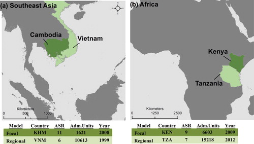
We compare population datasets produced for two countries (Cambodia [KHM] and Kenya [KEN]) using different training data: country-specific data (hereafter called focal model or F-model) and regional data (regional model or R-model). Cambodia and Kenya (Figure 1) have high level administrative unit census data, providing detailed focal country census units to be used for validation, but also share a border with countries that also have comparably high spatial resolution census data (Vietnam [VNM] and Tanzania [TZA], respectively). These neighboring countries were used for parameterizing and testing the regional model (R-model) for each country, respectively. To compare model structure and accuracy of the mapping outputs we generated a suite of population datasets by aggregating census units across a range of spatial resolutions for the focal country, while leaving the neighboring region country's data at its highest spatial resolution. Random forest models were estimated using focal-only data yielding the focal model (F-model), the focal model + regional model (F + R model) and the regional-only model (R-model) for each study area, the details of which are outlined below.

Data construction for focal and regional models

The focal models (F-model) use a suite of default covariate data layers (Stevens et al. in press) as well as additional country-specific data layers to estimate the population density weighting layer. The default data are comprehensive, contemporary datasets, most of which are freely available (Table 1). These data represent continuously varying properties across the landscape and are consistently mapped at a global scale. To complement these datasets, we also incorporate country-specific geospatial data that may correlate with human population presence on the landscape such as facility locations (e.g. health clinics, hospitals, schools). The availability of these data may vary widely country-by country. In addition, data from OpenStreetMap (OSM) (http://download-int.geofabrik.de/osm/asia/), an open source product that provides free worldwide geographic datasets, are used where appropriate for added information on infrastructure within countries such as buildings, settlements, residential areas, transportation networks, and water features (e.g. rivers, lakes, streams; Haklay and Weber 2008). If finer and more accurate, reliable, and clearly documented data exists from other in-country sources, these data are used in place of the OSM data. Complete metadata files are compiled for each country.

Table 1. Default data used in the R-model (regional model) of estimating population distribution.

Data	Description	Source
SRTM-based HydroSheds	Digital elevation data and its derived slope estimates	(Lehner et al. 2006)
WorldClim/BioClim	Mean annual precipitation (BIO12) and mean annual temperature (BIO1) estimates (1950–2000)	(Hijmans et al. 2005)
MODIS-derived, MOD17A3	Estimates of net primary productivity (NPP)	(Running et al. 2004)
Suomi National Polar-orbiting Partnership (NPP) Visible Infrared Imaging Radiometer Suite (VIIRS)	Observed lights at night standardized and provided as a global coverage	(NOAA 2014)
World Database on Protected Areas (WDPA)	Protected areas	(IUCN and UNEP 2014)
MODIS 500m Global Urban Extent	Global urban land c. 2001–2002	(Schneider, Friedl, and Potere 2009, 2010)

The countries selected for the R-model are neighboring, physically, and culturally similar countries that have more detailed census information and are used to parameterize the model estimation of population density. However, the neighboring countries may not include geospatial data at the national level that is comparable to the country of interest. Having an identical set of data between the neighboring countries and the focal country is required to share the random forest models between countries, as the ensemble of trees must include the same set of covariates for calibration and prediction – i.e. parameterizing a model on a set of covariates for one country, then applying it to another country requires identical types of covariate layers to be available for the application country. Therefore, the R-model might include a reduced, more general set of covariates than would be used for a country-specific parameterization. In the case studies presented here the standard default data (Table 1) and OSM datasets for each country are used. For the East African example, available health facility data was also incorporated into the model. Using these data the R-model can then be used in place of or in conjunction with the F-model to estimate the predicted population density layer that becomes the weighting layer in the dasymetric process of redistributing population counts for the focal country.

Random forest population modeling

Previous work provides an in-depth overview of the modeling framework (Stevens et al. in press; WorldPop 2014) but a short review is given here. Population data are acquired country-by-country at the finest spatial resolution publically available. These data are matched with other social and environmental ancillary datasets for use in a spatially-explicit population distribution model. All data is processed to ensure projections, resolutions, and extents match and that any ancillary data being used as covariates (ex. distance-to variables) are correctly calculated. These covariates are aggregated by administrative units and used in a semi-automated random forest predictive model (Breiman 2001; Liaw and Wiener 2002) to estimate a population density weighting layer at a spatial scale finer than that of the census data used for parameterization. The prediction density layer is then used in a dasymetric model to redistribute the census population counts.

The ‘random forest’ approach is characterized by using an ensemble of individual classification or regression trees which is advantageous in its flexible, nonparametric design (Breiman 2001; Liaw and Wiener 2002). As an ensemble classifier the ‘random forest’ model generates a final prediction based on an average of estimates from multiple individual regression trees. Each individual regression tree is a predictive model that uses a set of binary rules to calculate a predicted value and may be used either for classification or regression purposes. The predictors may be diverse, ranging from numerical to categorical, and incorporating both linear and non-linear relationships. The predictors, garnered from the best ancillary data sources available, may be included in different combinations across the many regression trees in the forest, chosen at random, and used to estimate the weighting layer using only the combinations proven to increase out-of-bag prediction accuracy. Predicted population density is estimated at the spatial scale of the covariates (typically ~100 m pixel sizes). This population density layer at the country level is then used as a weighting layer for the standard dasymetric mapping approach described by Gaughan et al. (2013) and Linard et al. (2012). The individual cell values of the resulting population maps represent people per pixel and people per hectare. Model estimation, fitting and prediction were completed using the statistical environment R 3.0.1 (R Core Team 2014) and the random forest package 4.6–7 (Liaw and Wiener 2002). The dasymetric portion of the model was written in Python 2.7 and used the arcpy ArcGIS geoprocessing facilities (ESRI 2011).

Statistical comparison approach

For all model estimations, we created multiple levels of aggregation, dissolving neighboring administrative units, and summing their population counts starting with the finest level of census data for each focal country. At each level of aggregation we conducted an iterative process, randomly selecting an existing administrative unit from the next lowest level of aggregation to merge with its neighbor with the longest shared border. If no neighboring units were available (e.g. an island), then the randomly selected unit was dissolved with the nearest unit. This process was iterated until one third of the units at the current level of aggregation had been dissolved, thereby reducing the number of units at the new level by one third. We chose to use one third as a compromise between using smaller steps of aggregation but increased computation time, and using larger levels of aggregation but having too few steps to accurately represent increases or decreases in mapping accuracy between those levels. By degrading the spatial units systematically we attempt to identify the ASR of the administrative unit data at which the R-model offers improved prediction accuracy over the F-country alone. The starting point was an ASR of 11 km, with a total of 1621 administrative units for Cambodia, and an ASR of 9 km, with a total of 6624 administrative units, for Kenya.

Predicted population density layers were produced using the random forest model, applied at each level of aggregation (e.g. for each ASR) and for both the F- and R-models. This was undertaken while keeping the ASR constant between the random forest and dasymetric parts of the model. We then compared the final mapping product from each combination to the finest level of census data available for the focal country by summing gridded population estimates within each administrative unit. Summary statistics were calculated for the combinations of observed and summed data, including root mean square error (RMSE), the RMSE divided by the mean census unit count (% RMSE) and the mean absolute error (MAE). These statistics are used to identify the intersection point between model approaches and thus determine a resolution threshold for when a regional model approach may be more appropriate than the focal model approach for estimating population distributions.

Lastly, to investigate how each model would respond to changes in ASR set independently for the random forest component and the dasymetric redistribution component of the model, we varied the ASR by holding the random forest ASR constant and changing the dasymetric ASR for each level of administrative unit aggregation for the focal country alone. The reason for conducting this analysis was to determine the importance of the input spatial resolution of the census data for the random forest model compared to the input census data used for ‘grounding’ the data in the dasymetric redistribution of population counts. Knowing that the ability to estimate a spatially-explicit redistribution of census data decreases with coarser administrative units, this process helps to identify how the decrease in ASR influences the fit of a random forest model. Validation statistics were calculated as above using RMSE, % RMSE and MAE.

Results

Overall, for countries with a large ASR (of around 55–60 km or larger), it may be more suitable to use a regionally-parameterized model (R-model). However, if the focal country census data is of fine ASR spatial resolution (of around 50–55 km or smaller; Figure 2), then the difference in RMSE across model types is minimal. This means that model transference to a regional dataset does not greatly improve on the focal country parameterization of the model. In situations where uncertainty exists about which model parameterization strategy is suitable, the use of the F + R model ensures that greater detail is drawn from the neighboring census units but additionally includes information specific to the country of interest.

Figure 2. Accuracy assessment results for (a) Cambodia and (b) Kenya for the Focal (F), Focal + Regional (F–R), and Regional (R) models plotted from coarser to finer-level census administrative units, as measured by ASR. Error is shown by the RMSE.

Model comparison varying ASR for population density prediction and dasymetric portions

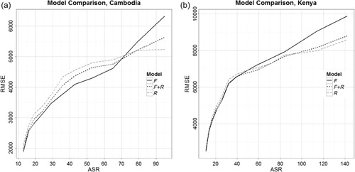
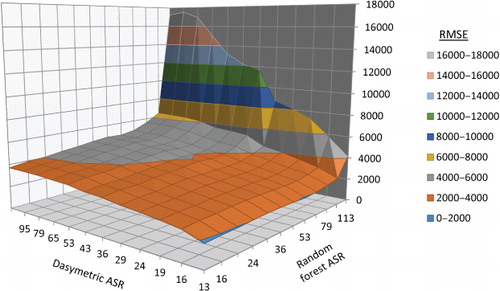
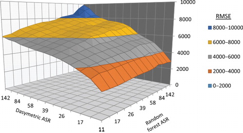
Varying the ASR helps identify how the level of detail in census input data influences the final model output. When changing the ASR for both the population density estimation and dasymetric components of the model by aggregating up, a shift begins to occur around an ASR of 50 km for Kenya and an ASR of 70 km for Cambodia in which the R-model is more accurate than the F-model (Figure 2). The lowest ASR value mapped for each country differed due to the total number of census units for each country. We did not run the modeling for less than 15 units as random forest or any other model estimation is unreliable for so few observations. At the coarser ASR levels (around 60 km or larger), the combination F + R model has a lower RMSE value than the F-model, performing similarly to the R-model. There does not seem to be much difference in RMSE values at finer ASR levels (around 30 km) suggesting that the use of the R-model improves model fit starting only at very low, coarse administrative units of focal data (around ASRs of 60-km). Figure 2 highlights how the prediction across models becomes more and more uniform with the increase in the number of total census units (i.e. decreasing ASR).

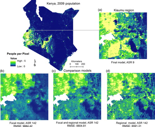
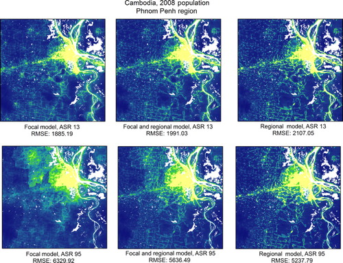
Figure 3 (Cambodia) and Figure 4 (Kenya) provide a visual comparison of the final predicted population distribution outputs that are based on the F-model and finest level ASR census data available for each country, to the population output for each model (F, F + R, and R) using the coarsest level ASR data. When limited to a coarser-resolution census dataset, the RMSE is lower for both countries and there is increased spatial detail with the use of the R-model. This is illustrated by the zoomed in portion of Phnom Penh and Kisumu regions (Figure 3d and Figure 4d). For a comparison of datasets using the finest and coarsest ASR levels mapped for Cambodia, Figure 5 illustrates the different visual patterns of each model (F, F + R, and R) zoomed in around Phnom Penh. At the coarsest ASR level (95), the best model is the R-model (RMSE 5238 compared to RMSE F-model = 5636 and RMSE F + R model = 6330) while at the finest ASR level (13km), the F-model has the lower RMSE (RMSE 1885 compared to RMSE R-model = 2107, and RMSE F + R model = 1991).

Figure 3. Illustration of different aggregated ASR units for the Phnom Penh region in Cambodia, highlighting the improved output of the random forest parameterization using census input from Vietnam in the (c) Regional model compared to the (a) Focal or (b) F + R models.

Figure 4. Illustration of different aggregated ASR units for the Kisumu region in Kenya, highlighting the improved output of the random forest parameterization using census input from Tanzania in the (c) Regional model compared to the (a) Focal or (b) F + R models.

Figure 5. ASR of the finest and coarsest levels used in generating the F-model, F + R model and R-model for Cambodia. RMSE values show that for the finest level ASR (13), the F-model performs the best while comparing the coarsest level ASR (95) identifies the R-model as having the lowest RMSE value.

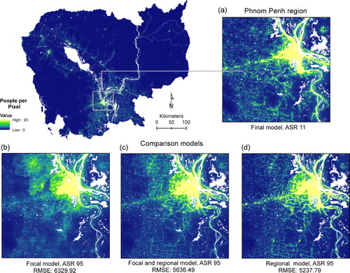
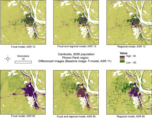
In order to quantify how the different spatial resolutions across models compare to the most current and accurate Cambodia dataset produced by WorldPop, which uses an ASR 11 km F-model (shown in Figure 2a), we calculated the difference between each of the example ASR outputs shown in Figure 4 and the model output. The ASR 11 km F-model represents the most current and accurate gridded population dataset produced by WorldPop. The difference between the population datasets is shown in Figure 5. Both the top and bottom rows show the F, F + R, and R model using an ASR of 13 km (relatively fine-scale), and 95 km (relatively coarse scale), respectively (Figure 5). The ASR 95 km models have a larger difference in population estimates between the base model (F-model, ASR 11 km) and each ASR 95 km model (bottom row) when compared to the ASR 13 km models (top row), with underestimation occurring in more dense, urban areas and the overestimation occurring in the more rural regions expanding out from Phnom Penh (Figure 6). These differences are less obvious in the finer-scale ASR outputs, with a more mixed pattern of over- and under-estimation occurring in the urban areas of Phnom Penh.

Figure 6. Differenced images for the finest and coarsest ASR levels generated for the Focal (F), Focal + Regional (F + R), and Regional (R) models. Each model output was subtracted from the final, ASR 9 F-model which represents the most current, up-to-date WorldPop population dataset for Cambodia.

Model comparisons keeping constant ASR for the population density estimation portion

Figures 7 and 8 provide more detail on the effect of ASR depending on whether it is the spatial resolution of the census data used in the dasymetric redistribution or the population density prediction model (in this case, a random forest model) estimation that influences the final population redistribution. The figures were constructed using the focal country data only, and allowing the aggregation of the census data used for dasymetric redistribution to vary independently from the census data used for random forest model estimation. The importance of the population density prediction part of the mapping is clear, and is starkly illustrated by the sharp decline in RMSE as the ASR decreases from maximal aggregation to even a few steps less aggregated. Though the ASR of the dasymetric and population density prediction components interacts it is clear, especially in Figure 7, that the effect on RMSE of varying the ASR of census units used for dasymetric mapping can be largely mitigated if small ASR census units are used for the population density prediction. In other words, if the census data for the focal country is coarser than the data used in the population density estimation (higher ASR) then we should favor a population prediction density model using lower ASR census data than the focal country.

Figure 7. Illustrates varying ASR for the population density estimation (e.g. random forest model) and the dasymetric step of the modeling process for Cambodia with increasing RMSE along the vertical axis.

Figure 8. Illustrates varying ASR for the population density estimation (e.g. random forest model) and the dasymetric step of the modeling process of the modeling process for Kenya with increasing RMSE along the vertical axis.

Discussion

Population maps are being used for risk assessment and policy-decision-making across a variety of fields but are limited by the availability of detailed, contemporary, and reliable census data The decision whether to incorporate information from areas other than the country of interest, where such data exist, has often been a subjective one (Linard, Gilbert, and Tatem 2011). Here we test for the first time the balance between regional and focal models and make initial steps toward developing quantitative rules in the modeling process. Results show that the ASR of census data plays a key role in the decision-making process of whether to parameterize the model at a regional level or use a more focal, country-specific parameterization in the redistribution of gridded population counts.

In this study, we compare the focal country model (F-model) to a regional model (R-model) and a combined focal + regional model (F + R model) generating a suite of comparison datasets across different levels of spatial aggregation for each model type. When coarser ASR census data is used as input into the model, parameterizing the population density prediction component is preferred using an R-model over an F-model. The R-model relies on finer-scale neighboring country census data to generate the population density prediction layer. In such a case, where the focal country census data is coarse, the R-model is able to use the larger number of input census units from the neighboring country and thus incorporate a larger range of variability in the population density estimation. Taking a more regional approach assumes that the model parameterized with data from outside the focal country is representative of the socio-environmental relationships measured between the covariates and population density of the focal country (Linard et al. 2010). Thus, when high ASR administrative data is available for the focal country and the scale of administrative units is detailed enough to provide a range of population densities across urban and rural areas, the F-model is preferable for fitting the model since we avoid potential biases introduced by those assumptions. Using the F + R model provides a measure of assurance of both the range in the variability of the predictor dataset and also confidence that the input data is representative of the area being mapped. Comparing the Cambodia and Kenya R-models to the F and F + R models (Figure 3(b) and 3(c), Figure 4(b) and 4(c), respectively,) highlights the improvement of using a regional model versus a focal model at coarse ASRs and how the average of the regional and focal models (R + F) will improve model output when the spatial resolution of census data is limiting for the country of interest.

Modeling techniques for estimating gridded population distributions based on national or subnational census inputs have increased in sophistication to use ancillary datasets and robust statistical techniques that more accurately redistribute population across spatial units (Balk and Yetman 2004; Tatem et al. 2007; Bhaduri et al. 2007; Wu, Qiu, and Wang 2005; Gaughan et al. 2013; Azar et al. 2013). Determining which statistical technique and which type of data are most informative to the estimation process is critical to choosing how to employ these sophisticated approaches. The example in this study uses a semi-automated random forest model which incorporates a larger suite of covariates than other methods (Gaughan et al. 2013; Linard et al. 2012) to generate the prediction density weighting layer that is then used to asymetrically redistribute the population across administrative units (Stevens et al. in press). The use of a random forest modeling approach improves on less complex weighting schemes, but more in-depth consideration is required with respect to how the population density prediction model reflects the quality and scale of the input data. One of the limitations of prediction density estimation models, such as the random forest model used here, is that the range of predictions is constrained by the variability of the training dataset (Strobl, Malley, and Tutz 2009). In mapping population estimates, smaller units typically relate to a larger range of population densities measured, which leads to a population density model that can encompass a greater range of variability and yield smaller numbers of people to redistribute within the census units weighted by that predicted population density layer. Thus, by using a census dataset from a neighboring country with a greater number of census units we can increase the amount of information used in the population density prediction. The F + R model provides even greater ranges of variability though if the F-model input data is extremely coarse then relying on the R-model data exclusively can result in a slightly better prediction output (Figure 2).

We investigated how varying the ASR influenced population density predictions and thus, final population outputs, by degrading the ASR of the input census data at multiple levels for the F, F + R, and R modeling approaches. The R-model was less sensitive to varying the ASR since the observed data used for the random forest and population density estimation remained at a constant, fine-scale level from neighboring census input data. However, the F and F + R models both varied in their population prediction density outputs as the number of F-model input census units varied across ASR levels. Figure 2 illustrates not only this process, identifying the robustness of the population density prediction model to the level of variability in training data, but also show a decrease in overall accuracy of the model, degrading linearly with the scale of census units used to ‘ground the data’ in the dasymetric portion of the model. This is more evident in Figures 7 and 8, which separate the two modeling steps to provide an indication of how well the overall model will perform based on the ASR of the census data used for either the population density prediction or dasymetric portion of the model.

Our results for both focal countries show that as you increase the ASR of the focal country relative to that of the R-model there is a crossover point at which the R-model begins to outperform the F-model. Unfortunately, this crossover point is not consistent between the two focal countries we tested. Our evidence suggests that there is likely not a simple ratio or factor of the difference between the F and R models that can be employed as a rule of thumb in all cases. An alternative hypothesis is that a correlation exists between the point at which the R-model outperforms the F-model based not on ASR but instead upon the range or variability encompassed in observed population densities of those administrative units for the F and R data. This range of population density is important primarily due to the nature of the random forest regression model. Inherent to its algorithm, random forest regression cannot predict outside the bounds of the data the model is parameterized on. Therefore, the larger the range or variability observed in the R-model relative to the F-model, we would expect the R-model to produce better results. In other words, as you aggregate census units the maximum and minimum of the observed population densities will regress toward the sum of the country as a whole, thereby decreasing variability in administrative unit counts. With less variability for the random forest model to be parameterized on, there will be a smaller range of predicted densities between rural and urban areas, decreasing the amount of dasymetric redistribution at the sub-census unit level. This is an area of active research and should be systematically tested across a broader range of contexts, but the mechanism we discuss here likely contributes indirectly to our results.

Determining the optimal training data for informing the process of population redistribution is important for minimizing the amount of error in the final population distribution datasets. This is especially relevant for some resource poor countries where contemporary, fine-scale census data may be limited. However, both the population prediction density layer and the final population maps rely on the accuracy and detail of the original census data. Error in the census data can propagate through the model process due to the amount of migration and movement within a population, the timing and accuracy of data collection, and uncertainties in population growth rates. Current research efforts are investigating alternative possibilities for circumventing the need for census data in population models, and include the use of very high resolution satellite data for building mapping combined with occupancy models (Vijayaraj, Bright, and Bhaduri 2007). It must also be noted that while the use of a population prediction density layer greatly improves the final gridded population estimates, there still remains a question as to the best way to assess the validity of the model input covariates. The random forest method provides a means to quantify the degree of uncertainty at the scale of census units but it is difficult to estimate the actual amount of uncertainty without sub-census validation data and this remains another area of promising active investigation in which micro-censuses and high resolution satellite imagery could be used as possible validation tools.

Lastly, consideration must be given toward the temporal and spatial aspects of using census data collected in one geographic area or time period to inform the mapping of distributions elsewhere and/or across years. In this paper we demonstrate the utility of applying neighboring census data of finer resolution for informing the population density prediction layer for a country of interest with coarser census data. However, cultural, ethical, and historical differences may mean that populations distribute themselves differently across a landscape depending on the location of a country or region. Current and future research should carefully consider these underlying aspects of a given population when modeling gridded population distributions. Temporally, there exists a need to explore the dynamics between changing landscape features and changing patterns in population distributions. Population growth and land cover change have occurred at unprecedented rates over the last half century, and as population models continue to be improved by availability of refined geospatial information, so must the approaches to how those data are used in the modeling process. The current modeling approach presented here relies on static covariate input layers into the prediction density model, and while not ideal, there now exists a long enough time period and technological capabilities to explore the changing relationships between population distributions and landscapes more dynamically and should be a focus of future research.

Conclusion

Population data products differ in their modeling approaches, whether predicting ambient population counts (Bhaduri et al. 2007; Dobson et al. 2000), or residential numbers (Gaughan et al. 2013; Linard et al. 2012; Balk and Yetman 2004), or use more novel techniques that take advantage of volunteered geographic information or other data generated by information and communication tools such as mobile phones or geotweets (Bakillah et al. 2014; Deville et al. in press; Goodchild and Glennon 2010; Reades, Calabrese, and Ratti 2009; Pulselli et al. 2008). As a result, predicted population distribution datasets will all have varying degrees of accuracy and uncertainty, compounded by the reliability and resolution of the input census data. In construction of these spatially-explicit models, it remains important to take into account the best combination of input data and ancillary information for estimating human population distributions. In addition, transparency in the methods employed for generating datasets provides a vital component for end users to both understand and appropriately apply model outputs in subsequent studies.

Gridded population datasets continue to be incorporated widely into studies examining aspects of health, land change, and climate in the context of larger global environmental and economic changes, providing a vital contribution to the digital earth initiative. The base spatial denominator of gridded population provides a means to identify specific regions at risk, quantify burdens, and provide a valuable source of population information to inform land change studies and develop strategies towards sustainable management of coupled human-environment systems (Tatem 2014). Determining quantitative rules for defining accurate estimations of population distributions is a priority. The example presented in this study uses a random forest prediction model (Breiman 2001), but other ensemble methods may also provide viable alternatives to the estimation process (Dietterich 2000). This study highlights the advancement of statistical tool sets and considerations to the underlying data used in the process of generating gridded population datasets and illustrates how, for many countries, more accurate population maps can be produced through defining model parameters from neighboring regions where more detailed data exists.

Funding

This work was supported by the RAPIDD program of the Science and Technology Directorate, Department of Homeland Security, and the Fogarty International Center, National Institutes of Health; NIH/NIAID [grant number U19AI089674]; and the Bill and Melinda Gates Foundation [grant number OPP1106427], [grant number 1032350]. CL is supported by the Fonds National de la Recherche Scientifique (F.R.S./FNRS), Brussels, Belgium. This work forms part of the outputs of the WorldPop Project (www.worldpop.org.uk) and Flowminder Foundation (www.flowminder.org).

References

- Azar, D., R. Engstrom, J. Graesser, and J. Comenetz. 2013. “Generation of Fine-scale Population Layers Using Multi-resolution Satellite Imagery and Geospatial Data.” Remote Sensing of Environment 130: 219–232. doi:10.1016/j.rse.2012.11.022.
- Azar, D., J. Graesser, R. Engstrom, J. Comenetz, R. M. Leddy, N. G. Schechtman, and T. Andrews. 2010. “Spatial Refinement of Census Population Distribution Using Remotely Sensed Estimates of Impervious Surfaces in Haiti.” International Journal of Remote Sensing 31 (21): 5635–5655. doi:10.1080/01431161.2010.496799.
- Bakillah, M., S. Liang, A. Mobasheri, J. J. Arsanjani, and A. Zipf. 2014. “Fine-resolution Population Mapping Using OpenStreetMap Points-of-interest.” International Journal of Geographical Information Science. doi:10.1080/13658816.2014.909045.
- Balk, D., and G. Yetman. 2004. The Global Distribution of Population: Evaluating the Gains in Resolution Refinement. New York: Center for International Earth Science Information Network (CIESIN). Accessed July 15, 2012. http://sedac.ciesin.org/gpw/docs/gpw3_documentation_final.pdf.
- Balk, D. L., U. Deichmann, G. Yetman, F. Pozzi, S. I. Hay, and A. Nelson. 2006. “Determining Global Population Distribution: Methods, Applications and Data.” Advances in Parasitology 62: 119–156. doi:10.1016/S0065-308x(05)62004-0.
- Bhaduri, B., E. Bright, P. Coleman, and M. L. Urban. 2007. “LandScan USA: A High-resolution Geospatial and Temporal Modeling Approach for Population Distribution and Dynamics.” GeoJournal 69: 103–117. doi:10.1007/s10708-007-9105-9.
- Bhatt, S., P. W. Gething, O. J. Brady, J. P. Messina, A. W. Farlow, C. L. Moyes, J. M. Drake, et al. 2013. “The Global Distribution and Burden of Dengue.” Nature 496 (7446): 504–507. doi:10.1038/Nature12060.
- Breiman, L. 2001. “Random Forests.” Machine Learning 45 (1): 5–32. doi:10.1023/A:1010933404324.
- Deville, P., C. Linard, S. Martin, M. Gilbert, R. S. Stevens, A. E. Gaughan, V. D. Blondel, and A. J. Tatem. in press. “Dynamic Population Mapping using Mobile Phone Data.” Proceedings of the National Academy of Sciences.
- Dietterich, T. G. 2000. “Ensemble Methods in Machine Learning.” Multiple Classifier Systems 1857: 1–15.
- Dobson, J. E., E. A. Bright, P. R. Coleman, R. C. Durfee, and B. A. Worley. 2000. “LandScan: A Global Population Database for Estimating Populations at Risk.” Photogrammetric Engineering and Remote Sensing 66 (7): 849–857.
- ESRI. 2011. ArcGIS Desktop Release 10.0. Redlands, CA: Environmental Systems Research Institute.
- Foley, J. A., R. DeFries, G. P. Asner, C. Barford, G. Bonan, S. R. Carpenter, F. S. Chapin, et al. 2005. “Global Consequences of Land Use.” Science 309 (5734): 570–574. doi:10.1126/science.1111772.
- Gaughan, A. E., F. R. Stevens, C. Linard, P. Jia, and A. J. Tatem. 2013. “High Resolution Population Distribution Maps for Southeast Asia in 2010 and 2015.” Plos One 8 (2): e55882. doi:10.1371/journal.pone.0055882.
- Goodchild, M. F., and J. A. Glennon. 2010. “Crowdsourcing Geographic Information for Disaster Response: A Research Frontier.” International Journal of Digital Earth 3 (3): 231–241. doi:10.1080/17538941003759255.
- Goodchild, M. F., and N. S. N. Lam. 1980. “Areal Interpolation – A Variant of the Traditional Spatial Problem.” Geo-Processing 1 (3): 297–312.
- Haklay, M., and P. Weber. 2008. “OpenStreetMap: User-generated Street Maps.” Ieee Pervasive Computing 7 (4): 12–18. doi:10.1109/Mprv.2008.80.
- Halpern, B. S., S. Walbridge, K. A. Selkoe, C. V. Kappel, F. Micheli, C. D’Agrosa, J. F. Bruno, et al. 2008. “A Global Map of Human Impact on Marine Ecosystems.” Science 319 (5865): 948–952. doi:10.1126/science.1149345.
- Hay, S. I., A. M. Noor, A. Nelson, and A. J. Tatem. 2005. “The Accuracy of Human Population Maps for Public Health Application.” Tropical Medicine & International Health 10 (10): 1073–1086. doi:10.1111/j.1365-3156.2005.01487.x.
- Hijmans, R. J., S. E. Cameron, J. L. Parra, P. G. Jones, and A. Jarvis. 2005. “Very High Resolution Interpolated Climate Surfaces for Global Land Areas.” International Journal of Climatology 25 (15): 1965–1978. doi:10.1002/Joc.1276.
- IUCN and UNEP. 2014. “The World Database on Protected Areas (WDPA).” UNEP-WCMC 2012. Accessed May 6. http://www.protectedplanet.net.
- Jiang, L. W., and K. Hardee. 2011. “How Do Recent Population Trends Matter to Climate Change?”. Population Research and Policy Review 30 (2): 287–312. doi:10.1007/s11113-010-9189-7.
- Lehner, B., K. Verdin, A. Jarvis, and W. W. Fund. 2006. HydroSHEDS Technical Documentation. World Wildlife Fund. Washington, DC. http://hydrosheds.cr.usgs.gov.
- Liaw, A., and M. Wiener. 2002. “Classification and Regression by randomForest.” R News 2 (3): 18–22.
- Linard, C., V. A. Alegana, A. M. Noor, R. W. Snow, and A. J. Tatem. 2010. “A High Resolution Spatial Population Database of Somalia for Disease Risk Mapping.” International Journal of Health Geographics 9: 1–13.
- Linard, C., M. Gilbert, R. W. Snow, A. M. Noor, and A. J. Tatem. 2012. “Population Distribution, Settlement Patterns and Accessibility across Africa in 2010.” Plos One 7 (2): e31743. doi:10.1371/journal.pone.0031743.
- Linard, C., M. Gilbert, and A. J. Tatem. 2011. “Assessing the Use of Global Land Cover Data for Guiding Large Area Population Distribution Modelling.” GeoJournal 76 (5): 525–538. doi:10.1007/s10708-010-9364-8.
- Linard, C., and A. J. Tatem. 2012. “Large-scale Spatial Population Databases in Infectious Disease Research.” International Journal of Health Geographics 11: 1–13. doi:10.1186/1476-072x-11-7.
- McGranahan, G., D. Balk, and B. Anderson. 2007. “The Rising Tide: Assessing the Risks of Climate Change and Human Settlements in Low Elevation Coastal Zones.” Environment and Urbanization 19 (1): 17–37. doi:10.1177/0956247807076960.
- Mennis, J. 2003. “Generating Surface Models of Population Using Dasymetric Mapping.” Professional Geographer 55 (1): 31–42.
- Mondal, P., and A. J. Tatem. 2012. “Uncertainties in Measuring Populations Potentially Impacted by Sea Level Rise and Coastal Flooding.” Plos One 7 (10): e48191. doi:10.1371/journal.pone.0048191.
- NOAA. 2014. “VIIRS Nighttime Lights – 2012.” Earth Observation Group, National Geophysical Data Center, National Oceanic and Atmospheric Administration (NOAA). Accessed May 5. http://www.ngdc.noaa.gov/dmsp/data/viirs_fire/viirs_html/viirs_ntl.html.
- Noor, A. M., D. K. Kinyoki, C. W. Mundia, C. W. Kabaria, J. W. Mutua, V. A. Alegana, I. S. Fall, and R. W. Snow. May 17, 2014. “The Changing Risk of Plasmodium Falciparum Malaria Infection in Africa: 2000—10: A Spatial and Temporal Analysis of Transmission Intensity.” The Lancet 383 (9930): 1739–1747. doi:10.1016/S0140-6736(13)62566-0.
- Pulselli, R., P. Ramono, C. Ratti, and E. Tiezzi. 2008. “Computing Urban Mobile Landscapes through Monitoring Population Density Based on Cellphone Chatting.” International Journal of Design & Nature and Ecodynamics 3: 121–134. doi:10.2495/D&NE-V3-N2-121-134.
- R Core Team. 2014. A Language and Environment for Statistical Computing 2013. Accessed May 5. http://www.r-project.org/.
- Reades, J., F. Calabrese, and C. Ratti. 2009. “Eigenplaces: Analysing Cities Using the Space-Time Structure of the Mobile Phone Network.” Environment and Planning B-Planning & Design 36 (5): 824–836. doi:10.1068/B34133t.
- Robinson, T. P., G. R. W. Wint, G. Conchedda, T. P. Van Boeckel, V. Ercoli, E. Palamara, G. Cinardi, et al. 2014. “Mapping the Global Distribution of Livestock.” PLoS ONE 9 (5): e96084. doi:10.1371/journal.pone.0096084.
- Running, S. W., R. R. Nemani, F. A. Heinsch, M. S. Zhao, M. Reeves, and H. Hashimoto. 2004. “A Continuous Satellite-derived Measure of Global Terrestrial Primary Production.” BioScience 54 (6): 547–560. doi:10.1641/0006-3568(2004)054[0547:ACSMOG]2.0.CO;2.
- Schneider, A., M. A. Friedl, and D. Potere. 2009. “A New Map of Global Urban Extent from Modis Satellite Data.” Environmental Research Letters 4 (4): 11. doi:10.1088/1748-9326/4/4/044003.
- Schneider, A., M. A. Friedl, and D. Potere. 2010. “Mapping Global Urban Areas Using MODIS 500-m Data: New Methods and Datasets Based on ‘Urban Ecoregions.’” Remote Sensing of Environment 114 (8): 1733–1746. doi:10.1016/j.rse.2010.03.003.
- Stevens, F. R., A. E. Gaughan, C. Linard, and A. J. Tatem. in press. “Disaggregating Census Data for Population Mapping Using Random Forests with Remotely-sensed and Ancillary Data.” PLoS ONE.
- Strobl, C., J. Malley, and G. Tutz. 2009. “An Introduction to Recursive Partitioning: Rationale, Application, and Characteristics of Classification and Regression Trees, Bagging, and Random Forests.” Psychological Methods 14 (4): 323–348. doi:10.1037/A0016973.
- Tatem, A. J. 2007. “Effect of Poor Census Data on Population Maps.” Science 318 (5847): 43–43. doi:10.1126/science.318.5847.43a.
- Tatem, A. J. 2014. “Mapping the Denominator: Spatial Demography in the Measurement of Progress.” International Health 6 (3): 153–155. doi:10.1093/inthealth/ihu057.
- Tatem, A. J., S. Adamo, N. Bharti, C. R. Burgert, M. Castro, A. Dorelien, G. Fink, et al. 2012. “Mapping Populations at Risk: Improving Spatial Demographic Data for Infectious Disease Modeling and Metric Derivation.” Population Health Metrics 10: 8. http://www.pophealthmetrics.com/Content/10/1/8.
- Tatem, A. J., N. Campiz, P. W. Gething, R. W. Snow, and C. Linard. 2011. “The Effects of Spatial Population Dataset Choice on Estimates of Population at Risk of Disease.” Population Health Metrics 9: 4 http://www.pophealthmetrics.com/content/9/1/4.
- Tatem, A. J., A. J. Garcia, R. W. Snow, A. M. Noor, A. E. Gaughan, M. Gilbert, and C. Linard. 2013. “Millennium Development Health Metrics: Where Do Africa's Children and Women of Childbearing Age Live?” Population Health Metrics 11: 11. http://www.pophealthmetrics.com/content/11/1/11.
- Tatem, A. J., A. M. Noor, C. von Hagen, A. Di Gregorio, and S. I. Hay. 2007. “High Resolution Population Maps for Low Income Nations: Combining Land Cover and Census in East Africa.” Plos One 2 (12): E1298. doi:10.1371/Journal.Pone.0001298.
- United Nations. 2012. World Population Prospects: The 2012 Revision, Key Findings and Advance Tables. New York: United Nations Department of Economic and Social Affairs/Population Division 7.
- Vijayaraj, V., E. A. Bright, and B. L. Bhaduri. 2007. “High Resolution Urban Feature Extraction for Global Population Mapping using High Performance Computing.” Paper presented at Proceedings of 2007 IEEE International geosciences and remote sensing symposium, IGARSS. http://web.ornl.gov/sci/landscan/landscan_references.shtml.
- Vorosmarty, C. J., P. Green, J. Salisbury, and R. B. Lammers. 2000. “Global Water Resources: Vulnerability from Climate Change and Population Growth.” Science 289 (5477): 284–288. doi:10.1126/science.289.5477.284.
- Wesolowski, A., N. Eagle, A. J. Tatem, D. L. Smith, A. M. Noor, R. W. Snow, and C. O. Buckee. 2012. “Quantifying the Impact of Human Mobility on Malaria.” Science 338 (6104): 267–270. doi:10.1126/science.1223467.
- Wint, W., and T. Robinson. 2007. Gridded Livestock of the World 2007. Food and Agriculture Organization of the United Nations.
- WorldPop. 2014. World Pop: High Resolution, Contemporary Data on Human Population Distributions 2013. Accessed May 4, 2013. http://www.worldpop.org.uk/.
- Wu, S., X. Qiu, and L. Wang. 2005. “Population Estimation Methods in GIS and Remote Sensing: A Review.” GIScience & Remote Sensing 42 (1): 80–96. doi:10.2747/1548-1603.42.1.80.