A virtual globe-based vector data model: quaternary quadrangle vector tile model

Abstract

This study proposes a virtual globe-based vector data model named the quaternary quadrangle vector tile model (QQVTM) in order to better manage, visualize, and analyze massive amounts of global multi-scale vector data. The model integrates the quaternary quadrangle mesh (a discrete global grid system) and global image, terrain, and vector data. A QQVTM-based organization method is presented to organize global multi-scale vector data, including linear and polygonal vector data. In addition, tile-based reconstruction algorithms are designed to search and stitch the vector fragments scattered in tiles to reconstruct and store the entire vector geometries to support vector query and 3D analysis of global datasets. These organized vector data are in turn visualized and queried using a geometry-based approach. Our experimental results demonstrate that the QQVTM can satisfy the requirements for global vector data organization, visualization, and querying. Moreover, the QQVTM performs better than unorganized 2D vectors regarding rendering efficiency and better than the latitude–longitude-based approach regarding data redundancy.

Keywords:

• multi-resolution modeling
• discrete global grid system
• vector data organization
• tile-based reconstruction
• geometry-based rendering

1. Introduction

Former US Vice President Albert A. Gore articulated a vision of ‘Digital Earth’ as a multi-resolution, three-dimensional representation of the Earth that would make it possible to find, visualize, and analyze massive amounts of georeferenced information (Gore 1998). Since then, different virtual globes have appeared with their own approaches for structuring data. Incorporating precise representation of the spatial position of features, vector data is an important data type stored and managed in virtual globes. The Geographic Information System (GIS) capabilities of a virtual globe could be significantly extended if vector data could be efficiently stored, displayed, and queried (Wartell et al. 2003). Vector data enable the proper rendering of features at all resolutions with different colors to distinguish between features. Vector data also facilitate quantitative analysis and attachment of attributes to features.

In a virtual globe the terrains are massive, thus multi-resolution modeling is necessary to represent global-scale terrain data in order to reduce their geometric complexity and to achieve real-time rendering (Luebke 2003). Techniques for displaying 2D vector data in local areas on multi-resolution terrains have been extensively studied over the past decade (Schneider, Guthe, and Klein 2005; Schneider and Klein 2007; Vaaraniemi, Treib, and Westermann 2011; Wartell et al. 2003). However, multi-resolution modeling of global-scale vector data has gained less attention. How to better manage, visualize, and analyze massive global multi-scale vector data with 3D coordinates, generated from draping 2D vector data (e.g. roads, rivers, building footprints, countries, and provinces) onto multi-resolution 3D terrain, is a great challenge.

Since the discrete global grid systems (DGGSs) have excellent properties, including hierarchical structure and global addressability, they could serve as a foundation for multi-resolution modeling of global-scale vector data. The DGGSs can be used for dynamic paging of global-scale data in real time depending on viewpoint, so that only a few tiles are refreshed at each frame. The spatial partitioning functionality provided by DGGSs is also the basic technique for GIS analysis. The analysis can be done using a level of the multi-resolution vector model. The level can be chosen dynamically depending on the viewpoint or the size of analysis, or be specified by the client.

The 3D vector models deserve further research as few 3D visualization tools exist in conjunction with 3D vector analysis functions (Ellul and Haklay 2006). The few existing virtual globes with vector analysis functions usually perform spatial analysis using 2D vector data and then visualize the results in 3D. The 2D vector results have to match the global terrain surface at runtime. The matching process lowers the rendering performance due to the complex computations, especially for dense polygonal vectors (as demonstrated in Section 6.2). More importantly, simple 2D analysis sometimes cannot yield accurate results. For example, when planning to build roads in mountainous areas, the shortest 2D path might not be the shortest 3D path, due to the greatly undulating terrain. Since the roads have not been built yet, there is hardly any other way to decide the real shortest path except 3D vector analysis. The 3D vector analysis is also helpful for surface area measurement in mountainous areas.

Thus, a virtual globe-based vector data model, the quaternary quadrangle vector tile model (QQVTM), is proposed to provide better visualization and analysis to virtual globe clients. QQVTM is designed primarily for large-scale vector data. However, it can also serve small-scale vector data. Based on the quaternary quadrangle mesh (QQM, one of the DGGSs) with analogous cell shapes and areas for the entire sphere, QQVTM hierarchically partitions global vector data into quaternary quadrangle tiles with vector fragments stored in them. Besides the vector fragments, each tile holds the local terrain and textures. Since all the data are organized in the same QQM structure, we can easily get to the image, terrain, and vector data of the same region for rendering and analysis purposes. In addition, tile-based reconstruction algorithms are designed to search and stitch the vector fragments to reconstruct and store the entire vector geometries to support 3D vector queries and analysis. Through the integration of QQM and vector data, QQVTM can build indexes for massive global vector data to facilitate queries, and furthermore can effectively decrease redundancy of vector data to accelerate rendering.

2. Related work

2.1. 3D vector models

Zlatanova, Rahman, and Shi (2004) pointed out that it is impossible to design a 3D topological model suitable for all types of applications, due to the specific requirements of particular categories of applications. Thus, different vector models are designed to satisfy different requirements. These models use primitives in zero dimension (0D), 1D, 2D, and 3D to describe simple objects (e.g. point, line, surface, and body). However, 3D primitives are rarely used, since 0D, 1D, and 2D primitives are sufficient in many cases (e.g. for describing buildings).

The formal data structure (FDS; Molenaar 1990) was the first data structure to consider spatial objects as an integration of geometric and thematic properties, and was implemented by Shibasaki and Shaobo (1992) to maintain and visualize 3D city models. The TEtrahedral Network (TEN; Pilouk 1996) was introduced to overcome some difficulties encountered by 3D FDS in modeling objects with indiscernible boundaries, such as geological formations and pollution clouds. TEN was one of the few models with a real 3D primitive (tetrahedron). The Simplified Spatial Model (Zlatanova 2000) was designed to serve web-oriented applications where spatial queries need to be visualized on the screen as 3D models. It has only two primitives (node and face) and avoids the storage of a 1D primitive.

Most vector models have a 2D primitive (face) with an arbitrary number of nodes, but TEN has a 2D primitive (triangle) with three nodes. A triangle is the basic primitive used to approximate surfaces in many 3D rendering engines, such as OpenGL and Direct3D. The restriction on face descriptions in TEN may complicate modeling, but facilitates visualization. Thus, the triangle might be a better 2D primitive for 3D vector models, since it furnishes the data for 3D rendering.

2.2. Discrete global grid systems

Most existing DGGSs are based on regular polyhedra or geographic coordinate systems. The regular polyhedral DGGSs tessellate the sphere using triangular (Dutton 1996; Fekete and Treinish 1990), quadrangular (Cozzi and Ring 2011; Mahdavi-Amiri, Bhojani, and Samavati 2013; White 2000), or hexagonal cells (Ben, Tong, and Chen 2010; Mahdavi-Amiri, Harrison, and Samavati 2014; Sahr 2008; White, Kimerling, and Overton 1992). Most of these DGGSs use 1:4 refinement. Specifically, 1:2 refinement was implemented by Mahdavi-Amiri, Bhojani, and Samavati (2013) since it provides the smallest factor of refinement among the refinements and therefore creates a smooth transition among cells. These regular polyhedral DGGSs have excellent properties, including a hierarchical structure, similar cell areas and shapes, and global addressability. However, mapping from a polyhedron to a sphere is a complex process because most cell edges do not coincide with meridians or parallels in a polyhedral DGGS. Thus, it is difficult to clip and resample existing geographic data to build multi-resolution models using polyhedral DGGSs without a costly conversion process which results in a loss of precision.

The existing systems for multi-resolution modeling of global-scale vector data are mostly based on the common latitude–longitude grid (Deng et al. 2013; Wartell et al. 2003; Sun et al. 2010). Such methods partition global vector data into tiles hierarchically and build indexes for them. They are easy to apply to existing georeferenced vector data for organization and visualization purposes. However, the latitude–longitude grid cell areas become smaller toward the poles. In addition, the shape of the cells becomes increasingly distorted and turns into triangles at the poles. The irregular cell areas and shapes result in data redundancy when organizing terrain data, due to overcrowding and repeated sampling points in high latitudes. For example, the elevation of the poles is repeated 43,200 times in GTOPO30 (U.S. Geological Survey 1999), which uses the latitude–longitude grid system. Hence, the redundant terrain data lead to redundant 3D vertices when incorporating 2D vector data, since the vectors have to intersect with redundant terrain grids. This data redundancy is an obstacle to efficient rendering and analysis in virtual globes.

Attempts have been made to create adjusted latitude–longitude grid systems to obtain more consistent cell sizes (Beckers and Beckers 2012; Bjørke et al. 2003; Bjørke and Nilsen 2004; Ma et al. 2009; NIMA 2003; Ottoson and Hauska 2002). Sun et al. (2009) proposed the Degenerate Quadtree Grid (DQG) with longitude intervals that increase regularly from the equator to the poles and latitude intervals that remain the same. The DQG has attractive properties, including a hierarchical structure, convergent geometrical distortion, and simple cell adjacencies. The DQG has solved the problem (to some extent) of large grid area and shape distortions at high latitudes. However, the polar grids are degenerated from quadrangles to triangles. These results indicate the occurrence of polar singularities that negatively affect the organization of polar data.

2.3. 3D vector visualization methods

Methods for displaying 2D vector data on 3D terrains can be broadly divided into three classes: texture-based, geometry-based, and shadow volume-based approaches. The texture-based approach has been widely used in earlier research (Kersting and Dollner 2002) and by existing virtual globes. This approach rasterizes the vector data into textures and overlays textures onto the terrain surface using texture mapping techniques. Since this approach rasterizes vector data into textures in a preprocessing step, it eliminates runtime operations to drape the vector data onto 3D terrains. The main drawbacks of this approach are that: (1) the accuracy of the mapping is limited by texture resolution resulting in aliasing artifacts (Schneider and Klein 2007); (2) much of the vector data will be filtered away when zooming out on the 3D terrains (Agrawal, Radhakrishna, and Joshi 2006); and (3) the additional information for vector data, such as identifying information, is lost after rasterization. The former two drawbacks lower visual quality. The third drawback strips vector data of its most important quality, the ability to support interactive operations and spatial analysis. Thus, the virtual globes using the texture-based approach have limited usefulness for the analysis of global-scale data (Goodchild et al. 2012).

To avoid these shortcomings, Wartell et al. (2003) proposed a geometry-based approach, creating geometry from the vector data by draping it onto the terrain surface. The accuracy of vector geometry generated by this approach is independent of the textures used and is, therefore, not limited to texture resolution. This approach produces higher quality and more flexible visual results, for example by assigning a unique color for chosen vector geometry. What is more, this approach can better support interactive operation and spatial analysis since it keeps the original properties of vector data. Thus, the geometry-based approach has been widely used by researchers (Agrawal, Radhakrishna, and Joshi 2006; Bruneton and Neyret 2008; Qiao et al. 2011; Schilling, Basanow, and Zipf 2007; Schneider, Guthe, and Klein 2005; Sun et al. 2010). However, the research has mainly aimed at linear vector rendering, and has barely dealt with polygonal vector rendering. The few published articles involving polygonal vector rendering are based on Triangular Inregular Network (Schneider, Guthe, and Klein 2005). The latitude–longitude grid system, which is more suitable for virtual globe applications, still lacks research.

A shadow volume-based approach, recently introduced by Schneider and Klein (2007), uses the stencil shadow volume algorithm to create a pixel-exact draping of vector data onto terrain models. This approach extrudes the vector geometry into polyhedra that are afterward rendered into the stencil buffer to generate an appropriate mask. This approach is independent of the underlying terrain geometry and utilizes a high-performance rendering engine. Since the method is a screen-space algorithm, it allows high-quality real-time overlaying of vector data on 3D terrains and does not suffer from aliasing artifacts. However, this method cannot easily support quantitative analysis, such as 3D optimum route analysis, since the elevation of every vertex in vector data is not calculated. Meanwhile, Vaaraniemi, Treib, and Westermann (2011) demonstrated that the geometry-based method can deliver higher rendering performance than the shadow volume-based method.

Existing research has mainly aimed at rendering vector data for local areas, and has barely dealt with the multi-resolution modeling of global-scale vector and terrain data. Few have integrated DGGS, multi-resolution terrain models, and vector data to achieve a virtual globe-based multi-resolution organization and visualization of vector data. Therefore, this paper proposes a vector data model, QQVTM, which organizes vector data using QQM and visualizes it using a geometry-based approach. Our method guarantees rendering accuracy and efficiency and retains the additional information found in vector data. Organized vector data with 3D coordinates and additional information can lay the foundation for vector data queries and 3D quantitative analysis in a virtual globe environment.

3. Data model

3.1. Quaternary quadrangle mesh

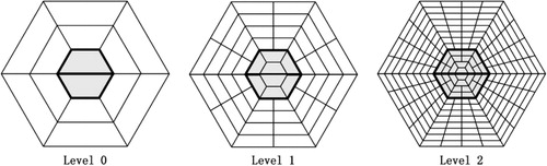
Zhou, Chen, and Gong (2013) proposed a pole-oriented DGGS, referred to as the QQM. The QQM uses semi-hexagon (a type of quadrangle) grids for the polar regions and rectangular grids elsewhere (Figure 1). At each lower level, the two polar cells in each hemisphere were divided into four smaller child semi-hexagons respectively, and other cells were recursively and equally divided into four smaller child rectangles by degrees. Semi-hexagonal partitioning in the polar regions reduces the redundancy in polar data and avoids the polar singularity that frequently exists in DGGSs. A consistent encoding–decoding scheme and a uniform adjacent search algorithm were constructed by considering that polar cells and other cells form a coherent and seamless unity in the QQM, which has a hierarchical structure.

Figure 1. Recursive subdivision of the QQM hemisphere.

3.2. Quaternary quadrangle vector tile model

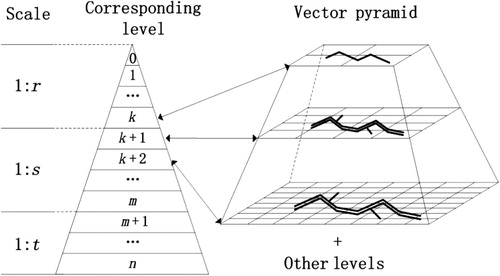
There are massive amounts of vector data and corresponding terrain and image data to be rendered and analyzed in a virtual globe. Loading all the data into memory at once will consume substantial computing resources resulting in poor performance of rendering and analysis, and is likely to end up with an out-of-memory exception. To efficiently manage and visualize massive global vector data with 3D coordinates, generated from draping 2D vector data on the 3D terrain surface, a global multi-resolution vector data model is necessary. Thus, we propose a virtual globe-based vector data model, the QQVTM (Figure 2). The QQVTM consists of three parts (Figure 2a):

Figure 2. (a) Conceptual model for QQVTM and (b) Logical model of QQVTM. Note: Rectangles represent entity sets and ovals represent attributes. Diamonds with lines connecting to entity sets represent containing or constitution relationships between two entity sets (e.g. a tile contains n vertices and n arcs constitute a boundary). The numbers on the lines indicate three kinds of quantitative relationships: (1) 1:1 indicates a one-to-one relationship, (2) 1:n indicates a one-to-many relationship, and (3) m:n indicates a many-to-many relationship. To implement a relationship between two objects, the key of one attribute table is included in the other attribute table. The associated keys are linked using lines.

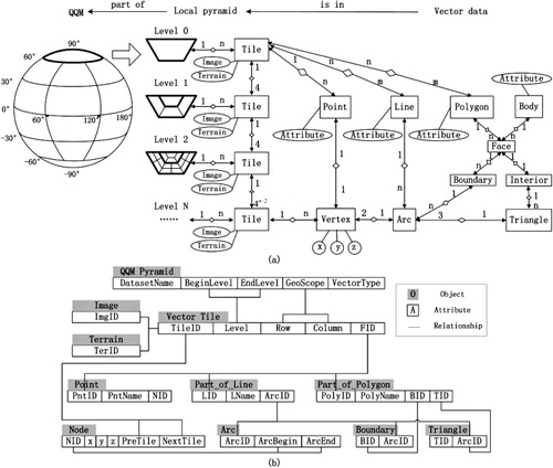
1. The QQM. It is used to partition the sphere hierarchically. To handle required data flexibly, we partitioned the global vector data into levels and tiles and built indexes for them using QQM. The tiles were regarded as part of the model.

2. A local pyramid. It is a multi-resolution representation of a partial region in the QQM and contains vector tiles with vector fragments stored in them. A vector tile is associated with corresponding image and terrain data through the same ID. The tile number in level N quadruples the tile number in level N–1. The pyramid structure is used for dynamic paging of data in real time depending on viewpoint, so that only a few tiles are refreshed at each frame. Building multi-resolution models for different vector data produces different local pyramids. The QQVTM involves four kinds of vector data: point, line, polygon, and body.

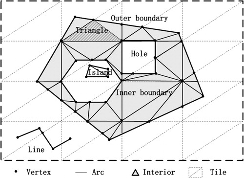
3. The vector data (Figure 3). The vertices with 3D coordinates and adjacency information are the fundamental elements of vector data. A vertex and additional attributes comprise a point. Two vertices connect to form an arc. One or more arcs compose a line or a boundary of a polygon. A polygon has one or more faces (sub-polygons) in a tile, and a body has several faces. Each face has one outer boundary and may have several non-nested inner boundaries, i.e., may have holes or islands. Between the outer and inner boundaries is the interior of the face. The interior is represented as triangles, since the triangle is the basic primitive used to approximate surfaces in many 3D rendering engines, such as OpenGL and Direct3D. Each triangle consists of three arcs. The boundaries indicate the geographical scope of a polygon and are mainly used for analysis. The interior triangles are mainly used for surface rendering. A vector geometry is divided into vector fragments, related with each other through the same FID (PntID, LID, or PolyID), and stored in different vector tiles. A body object (e.g. buildings) often has a small geographical span and does not need to be clipped into tiles. Only its footprints need to match the multi-resolution terrain to produce the multi-resolution body model. Hence, body objects will not be discussed in this paper.

Figure 3. Vector data in QQVTM.

The QQVTM combines tile objects and vector objects, and integrates the attribute information and corresponding image and terrain data. It realizes integrated management and visualization of global multi-resolution vector, terrain, and image data by organizing all the data into the same QQM structure.

4. Organization of vector data

4.1. Matching with multi-resolution terrain

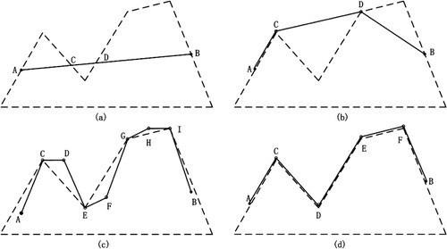
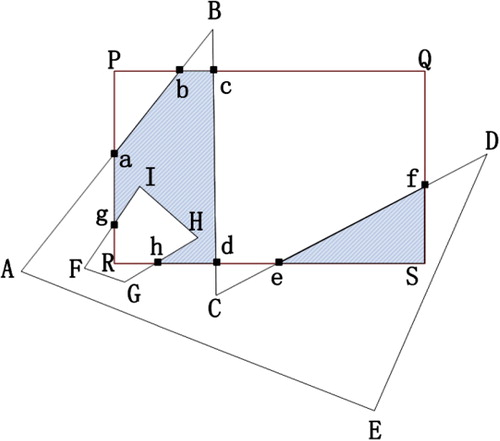
When rendering vector data on multi-resolution 3D terrain, simply mapping the vertices contained in the vector data is not sufficient and will lead to overhanging (CD in Figure 4a) and hidden landscape (AC in Figure 4a) parts. Even if the vector data are mapped to a level of the multi-resolution terrain model, when the terrain level changes and the resolution of a vector tile is lower or higher than the resolution of underlying terrain data, there will be sunken (DB in Figure 4b) and raised (CD in Figure 4c) parts. Thus, to make the vector data with 3D coordinates stick to the terrain surface, the original 2D vector data have to be first integrated with the multi-resolution terrain data to create vector pyramids. Then, vector and terrain data of the same resolution are fetched during rendering (Figure 4d). A tile is limited to using only one LOD level, and two neighboring tiles cannot have an LOD difference larger than one.

Figure 4. Geometry-based mapping of vector data. (a) Simply mapping the vertices contained in the vector data. (b) The resolution of the vector tile is lower than the resolution of the underlying terrain data. (c) The resolution of the vector tile is higher than the resolution of the underlying terrain data. (d) The vector geometry conforms closely to the terrain surface since they have the same resolution.

Visual cracks in terrain data exist at the joints of two banks and the joints of two LOD levels, due to the different longitude or latitude spans of cells. These terrain cracks lead to bank cracks and LOD cracks of vectors (Figure 5a). Two alternative methods are available for eliminating these cracks: (1) adding vertices into cells of larger longitude spans (Figure 5b) and (2) removing vertices from cells of smaller longitude spans (Figure 5c). However, the two ways available for realizing the first method complicate operations: (1) store the added vertices in border tiles at the expense of a complicated storage structure since the border tiles are different from other tiles; (2) add a pointer to the neighbor tile with a smaller longitude span for each tile with a larger longitude span and then read the data stored in neighbor tiles during rendering. We chose to implement the second method, which does not require modification of the storage structure or require reading of neighbor tiles and therefore has higher rendering performance.

Figure 5. Elimination of visual cracks.

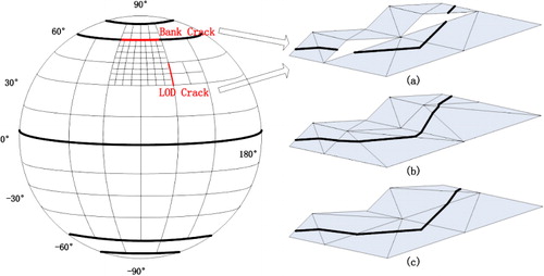
The bank cracks can be eliminated in preprocessing, owing to their fixed positions. The LOD cracks can only be eliminated during rendering, since their positions change with the viewpoint. However, in all cases while testing our system the number of LOD cracks that occurred in one frame was very low. It is more efficient to adjust only the vectors at LOD cracks than to match all the vectors to the terrain at runtime.

4.2. Vector pyramid

The original 2D vector data were mainly generated from vectorizing existing surveying and mapping results. The vector data at different scales were produced to satisfy different demands; they express features at different detail levels and have different degrees of generalization. A feature at different scales has a distinctive accuracy and even varies in shape. For example, a river represented by a single curve in small-scale vector data can be expressed using its two boundaries and branches in large-scale vector data. Therefore, even if small-scale vector data are draped onto high-resolution terrain data, the results will still deviate due to inaccuracies in the X–Y plane. The results cannot match the high-resolution image data properly or express required details of the feature. Conversely, if large-scale vector data are used to produce low-resolution tiles, unnecessary or unwanted geometric detail will overcrowd the rendering results and lower the visual quality. In general, the scale of vector data determines the vector pyramid levels it can construct. The max QQM level vector data can produce is calculated as follows:

The approximate quantitative relationship between scale and resolution is

(1)

where PPI = 96 is the pixel per inch of a normal computer screen and C = 0.0254 is the conversion constant from inch to meter.

The longitude resolution of a QQM level can be calculated using the formula (Zhou, Chen, and Gong 2013):

(2)

where R = 6,371,004 m, the average radius of Earth; L is the QQM level; and P is the pixels per tile in the longitudinal direction (P = 32 in our experiment).

From formula (1) and (2), the max QQM level is:

(3)

where the symbol ‘int’ indicates that the value is rounded down.

By combining the vector pyramid levels generated from different scales of a feature class, a complete vector pyramid of the feature class was built (Figure 6).

Figure 6. Vector pyramid (r > s > t and k < m < n).

After the levels of a vector pyramid are determined, the 2D vector data were draped onto multi-resolution terrain data to create a vector pyramid using the algorithm below:

begin

for (each level)

{

 calculate the rows and columns using the geographical scope according to Zhou, Chen, and Gong (2013)

for (each tile)

{

fetch the terrain data with TerID (level, row, and column)

If (polygon data)

{

  clip the polygon data using the Weiler-Atherton clipping algorithm (Weiler and Atherton 1977, Figure 7) to get the sub-polygons within each terrain cell

  triangulate the sub-polygons to get the triangles that represent the interior of the polygon

  calculate the elevations of the triangle vertices to get the complete 3D coordinates and store the 3D vertices into the tile

}

else if ( line data)

{

  clip the line data using the Cohen-Sutherland clipping algorithm to produce vector fragments

  calculate the intersections of the 2D vector fragments and plane terrain grids

  calculate the elevations of the intersections and original vertices to get the complete 3D coordinates and store the 3D vertices into the tile

}

write the tile into a dataset

}

}

end

Figure 7. The Weiler–Atherton clipping algorithm can clip all polygons, including concave polygons and polygons containing holes. The boundary of the clipping result of a polygon (abcdhHIga) constitutes a partial polygon boundary (ab, cd, and hHIg) and a partial tile boundary (bc, dh, and ga).

5. Tile-based reconstruction of vector data

In a vector pyramid, tiles in level 0 contain the most unbroken vector geometries. As the level number increases, the quantity of vector geometries contained in a single tile gradually decreases, and the vector geometries are turned into smaller vector fragments. These vector fragments are prone to disconnection during reconstruction. Linking these fragments to reconstruct and store the entire vector geometries to support vector querying and 3D analysis is an important problem, to be solved at the data organization stage.

Tile-based reconstruction of vector data refers to the process of searching the vector fragments scattered in several tiles and stitching the fragments together to reconstruct entire vector geometries. The key to reconstruction is seeking out the vector fragments and obtaining the vertex series according to the link relationships of vector tiles.

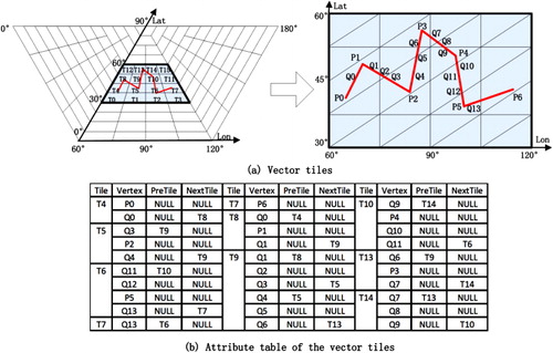
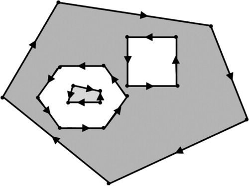
The link relationships of vector tiles are generated in the data organization stage and recorded in temporary tables using the PreTile and NextTile items of the intersections of vector data and the QQM cell boundaries (Figure 8b). The temporary tables are deleted after the reconstruction stage. PreTile is the previous neighboring tile of the current tile and NextTile is the next tile of the current tile when traversing the vector data. The PreTile and NextTile items contain the orientation and adjacency information of vector data and invoke the integrity of vector geometries. If the PreTile or NextTile of a vertex in a tile is not null, the vertex is an intersection of vector data and the tile boundary, which indicates fragments of the vector geometry in a neighbor tile (Figure 8). If the PreTile is not null, the vertex is an ‘in-vertex’ of the vector geometry in a tile (Q1 of T9 in Figure 8). If the NextTile is not null, the vertex is an ‘out-vertex’ of the vector geometry in a tile (Q6 of T9 in Figure 8). Otherwise, the vertex is an inner vertex of the vector geometry in a tile (Q5 of T9 in Figure 8).

Figure 8. Tile-based reconstruction of vector data. P0, P1, … P6 are the original vertices of the 2D vector data. Q0, Q1, … Q13 are the intersections of the 2D vector data and the terrain grids. (a) Vertices are stored in tiles. (b) The link relationships of vector tiles are recorded in temporary tables using the PreTile and NextTile items of the intersections.

Tile-based reconstruction algorithms of polygons and lines are presented. For a polygon, the interior and the boundaries are handled separately. Since the interior triangles are mainly used for rendering, the orders of triangles are not that important; we only need to seek out the triangles belonging to a polygon according to their FIDs. The boundaries are reconstructed through the same algorithm with line reconstruction:

begin

 the selected tile=>current tile

 FirstHalf:

   search for the first in-vertex of FID sequentially in the current tile

   if (no in-vertex exists) goto Invert

   else

   {

     PreTile of the first in-vertex=>current tile

     null=> PreTile of the first in-vertex

     search for the last in-vertex reversely in the current tile

     store the vertices passed into the vertex array

     goto FirstHalf

   }

Invert:

   invert existing vertex array

   the selected tile=>current tile

SecondHalf:

   search for the first out-vertex sequentially in the current tile

   if (no out-vertex exists) goto end

   else

   {

     store the vertices passed into the vertex array

     NextTile of the first out-vertex=>current tile

     null=> NextTile of the first out-vertex

     goto SecondHalf

   }

end

Tile-based reconstruction algorithms can deal with a scenario where a vector geometry enters and exits a tile several times. The PreTile of the first in-vertex and the NextTile of the first out-vertex are cleared after the first use to avoid reuse. The results of reconstruction are stored in tables separately from the tiles to support vector queries and 3D analysis. The lines and outer boundaries of polygons are stored in a clockwise order; the inner boundaries of polygons are stored in a counterclockwise order. The storing order guarantees that the interior of a polygon is always on the right of the forward direction when traversing a vertex list (Figure 9).

Figure 9. Storing order of polygon boundaries. Note: The dashed area is the interior of the polygon, which is always on the right of the forward direction when traversing a vertex list.

6. Experiments

The experiments were performed at a display resolution of 1280 × 1024 on a PC with an Intel Core 2 3.1 GHz processor with 3.2 GB of RAM and an NVIDIA Quadro 600 graphics card.

6.1. Visualization and interaction

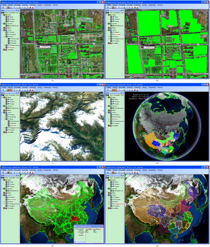
To show the validity of QQVTM, the following data were organized using QQVTM and visualized using C++ and Direct3D: (1) linear vector data for global national boundaries and rivers, roads, and railways in China; (2) polygonal vector data for provinces in China and footprints of buildings in Taizhou city; (3) global terrain data at a resolution of 90 meters; and (4) global Blue Marble data at a resolution of 1000 meters and image data of Taizhou city at a resolution of 0.6 meters.

The QQVTM uses a simple structure with smooth visualization, especially in the polar regions. It fills the gaps in the organization and visualization of global-scale 3D polygonal vectors (Figure 10). The vector data match with the image data well, with few deviations (Figure 10c). The deviations are inherited from the inaccuracies of the original 2D vector data and are by no means due to deficiencies of our method. Banks with different cell longitude spans stitch seamlessly at the borders (the red circle in Figure 10d). In addition, the vector geometries can be picked interactively and then highlighted with their attributes shown (Figure 10e), and the color of vector geometries can be changed interactively (Figure 10f).

Figure 10. Renderings of organized global vector, terrain, and image data based on QQVTM.

6.2. Performance test

6.2.1. Pyramid building performance

The linear (77,843 original vertices) and polygonal (90,340 original vertices) data for provinces in China were used to test the performance of building vector pyramids based on the QQM. The time consumption and vertex increase of levels 0–4 are shown in Table 1. The time consumption of preprocessing linear and polygonal data nearly doubled and quadrupled, respectively, with each level increase, since lines are 1D and polygons are 2D. The preprocessing of polygonal data consumed much more time due to the complex triangulation algorithm. For linear data, the vertex increase after the preprocessing was also doubled with each level increase. For polygonal data, the condition was much more complex, since the terrain vertices inside the polygon were inserted into it.

Table 1. Performance of building QQM vector pyramids.

	Line			Polygon
		Vertex increasing			Vertex increasing
Levels	Time (ms)	Number	Percentage	Time (ms)	Number	Percentage
0	262	2214	2.84	75,313	188,006	208.11
1	453	4318	5.55	263,078	216,986	240.19
2	766	8704	11.18	1,032,984	314,978	348.66
3	1125	17,448	22.41	4,128,625	668,558	740.05
4	1922	35,028	45.00	16,445,219	2,005,781	2220.26

6.2.2. Reconstruction efficiency

The vector pyramid of linear data built in Section 6.2.1 was used to test the efficiency of the tile-based reconstruction algorithm. The time consumption was nearly doubled with each level increase (Table 2). The results of reconstruction were stored in tables separately from the tiles and could be used directly in spatial analysis. The reconstruction was a preprocessing step in spatial analysis, and thus the efficiency of reconstruction will not affect the spatial analysis.

Table 2. Efficiency of the tile-based reconstruction algorithm.

Levels	0	1	2	3	4
Time (ms)	569	1109	2016	4406	11,953

6.2.3. Rendering performance comparison

The purpose of this experiment is to demonstrate the viewpoint we mentioned in Section 1 that draping 2D vector data onto a terrain surface at runtime lowers the rendering performance. The linear vector data for roads in China and the polygonal vector data for provinces in China were used in the performance test. The frame rates of rendering the organized 3D vectors and the un-preprocessed 2D vectors were then compared.

Table 3 shows the frame rates while flying 4000 km and 100 km above Earth's surface when rendering the quaternary quadrangle vector tiles. The frame rates were stable and similar when rendering organized 3D lines (roads), 3D polygons (provinces), and terrain. The vector data size has little influence on rendering performance, since the preprocessing prepared the 3D nodes and triangles for 3D rendering and thus eliminated the complex runtime computations.

Table 3. Frame rates of quaternary quadrangle vector tile rendering in 30 seconds.

Distance (km)	4000			100
Frame rate	Min	Max	Average	Min	Max	Average
Terrain	41	44	42.6	41	44	42.567
Lines	39	46	41.6	41	44	42.633
Polygons	42	44	42.7	41	44	42.6

Figure 11 shows the frame rates of rendering the unorganized 2D vectors directly. When rendering 2D lines and polygons while flying 100 km above Earth's surface, the average performance drop was about 18.61% and 45.07% compared to rendering organized 3D lines and polygons, respectively. When rendering 2D lines and polygons while flying 4000 km above Earth's surface, the average performance drop was about 82.21% and 96.18% compared to rendering organized 3D lines and polygons, respectively. The rendering performance dropped heavily with the rise of the viewpoint, due to the increased data size of visible vectors. A higher performance impact occurred over areas with denser vectors. Visible 2D lines had to be draped onto terrain and the intersections and elevations had to be calculated during rendering. Even more complex computations, including polygon clipping and triangulation, had to be done for the visible 2D polygons. Thus, it was hard to achieve real-time rendering with large amounts of visible 2D polygons.

Figure 11. Frame rates while flying 4000 km and 100 km above Earth's surface.

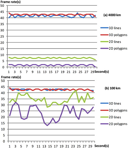
The result is that rendering organized 3D vectors has much higher frame rates than rendering un-preprocessed 2D vectors, especially for dense visible polygons.

6.3. Data size comparison

Lower data redundancy in a dataset improves the efficiency of processing and rendering. The improvement will be even more apparent in a network environment since the pressure of network transmission reduces together with the data size. However, the consistency of cell sizes is also an important indicator to evaluate whether a DGGS is suitable as the framework of a virtual globe. Thus, a DGGS with lower data redundancy and more consistent cell sizes is preferable. With a limited geometrical distortion and efficient encoding, decoding, and adjacent search performances (Sun et al. 2009), the DQG was chosen as an example of an adjusted latitude–longitude grid system to compare with the QQM. The latitude–longitude grid system is another comparison system.

Global terrain data at a resolution of 90 meters were organized into tiles of size 33 × 33, 49 × 49, and 33 × 65 using latitude–longitude grids, DQG, and QQM, respectively. The three terrain pyramids had the same lowest resolution (about 100 meters) and same highest resolution (about 100,000 meters). Vector data of global national boundaries including 247 polylines consisting of 241,271 vertices were also organized using latitude–longitude grids, DQG, and QQM to create vector pyramids by integrating 2D vector data with the terrain pyramids. The vector pyramids were set to have the same levels as the terrain pyramids in order to count the vertex numbers in each level. The data sizes of three vertex numbers of two vector pyramids are compared respectively in Table 4. Specifically, the vertex numbers of high latitudes ([−90 to −60] and [60 to 90]) and low latitudes ([−60 to 60]) in latitude–longitude grids and QQM pyramids are compared in Table 5.

Table 4. Data size comparison between terrain pyramids and vertex number comparison between vector pyramids.

		Vertex number
Levels	Resolution (m)	QQM	LLG	DQG	QQM/LLG (%)	QQM/DQG (%)
0	104,245	263,179	276,884	270,937	95.05	97.14
1	52,123	294,311	312,474	294,067	94.19	100.08
2	26,061	353,216	383,969	344,542	91.99	102.52
3	13,031	466,254	526,547	446,904	88.55	104.33
4	6515	691,893	813,244	652,744	85.08	106.00
5	3258	1,145,236	1,389,004	1,065,875	82.45	107.45
6	1629	2,053,978	2,544,637	1,893,221	80.72	108.49
7	814	3,874,091	4,858,509	3,550,610	79.74	109.11
8	407	7,516,503	9,488,208	6,867,040	79.22	109.46
9	204	14,801,592	18,748,168	13,500,942	78.95	109.63
10	102	29,371,442	37,268,072	26,770,257	78.81	109.71

LLG, latitude–longitude grids.

Table 5. Vertex number comparison between two vector pyramids at low and high latitudes.

	Low latitudes			High latitudes
Levels	QQM	LLG	QQM/LLG (%)	QQM	LLG	QQM/LLG (%)
0	170,451	170,536	99.95	92,728	106,348	87.19
1	191,764	192,001	99.88	102,547	120,473	85.12
2	234,693	235,134	99.81	118,523	148,835	79.63
3	320,519	321,378	99.73	145,735	205,169	71.03
4	492,242	494,534	99.54	199,651	318,710	62.64
5	837,561	842,542	99.41	307,675	546,462	56.30
6	1,529,793	1,541,235	99.26	524,185	1,003,402	52.24
7	2,915,547	2,939,979	99.17	958,544	1,918,530	49.96
8	5,688,400	5,739,437	99.11	1,828,103	3,748,771	48.77
9	11,233,883	11,337,470	99.09	3,567,709	7,410,698	48.14
10	22,324,719	22,533,943	99.07	7,046,723	14,734,129	47.83

LLG, latitude–longitude grids.

Table 4 indicates that (1) the ratio of the vertex number of a vector pyramid based on QQM and the vertex number of a vector pyramid based on latitude–longitude grids decreases gradually as the level number increases and becomes 78.81% at level 10 with a resolution of about 100 meters and (2) the ratio of the vertex number of a vector pyramid based on QQM and the vertex number of a vector pyramid based on DQG increases gradually as the level number increases and becomes 109.71% at level 10. Zhou, Chen, and Gong (2013) have proved that QQM has more consistent cell sizes than DQG. The larger data amount is the result of the smaller cell size in latitude 45 to 60, which is more approximate to the equatorial cell size. Thus, the QQM is still a good choice as the framework of a virtual globe even with a slightly larger data redundancy than the DQG.

Table 5 indicates that (1) the vertex number of a vector pyramid based on QQM is a little less than the vertex number of a vector pyramid based on latitude–longitude grids in low latitudes; and (2) the vertex number of a vector pyramid based on QQM is much less than the vertex number of a vector pyramid based on latitude–longitude grids in high latitudes; the former is only 47.83% of the latter at level 10 with a resolution of about 100 meters.

The data redundancy is reduced thanks to the rarefaction of the overcrowded terrain data in high latitudes of QQM, which leads to fewer intersections of vector data and terrain grids. The lower data redundancy in high latitudes improves the efficiency of processing and rendering.

7. Conclusions and future work

A virtual globe-based vector data model, QQVTM, was proposed in this study to integrate QQM (one of the DGGSs), 2D vector data, and 3D terrain data. QQVTM partitioned the virtual globe and built indexes for the tiles based on QQM. It incorporated multi-scale vector data with multi-resolution terrain pyramids to create a multi-resolution vector pyramid in the data organization stage. The QQVTM was constructed based on QQM with properties as follows:

1. Easy to apply to existing georeferenced data. The QQM uses a regular hierarchical structure and a simple relationship with latitude and longitude. Thus, QQM is easily used to clip vector data and manage corresponding terrain and image data.

2. Easy reconstruction of vector data. The vector fragments scattered in several tiles can be found and stitched to reconstruct the entire vector geometries according to the PreTile/NextTile of the intersections of vector data and QQM cell boundaries. The time consumption of the reconstruction algorithm is tolerable.

3. Low data redundancy. At a resolution of about 100 meters, the vertex number of vector pyramids based on QQM was 78.81% of the vertex number of vector pyramids based on latitude–longitude grids. The former was only 47.83% of the latter in high latitudes. Although the QQM pyramid had a slightly larger data redundancy than the DQG pyramid, QQM had more consistent cell sizes than DQG, which is an important indicator for evaluating DGGSs.

4. Efficient rendering. Rendering the organized 3D vectors had much higher frame rates than rendering the un-preprocessed 2D vectors, especially for dense visible polygons. Rendering the few visible vector tiles of small data size was much more efficient and less memory-consuming than rendering all global vector data. The lower data redundancy at high latitudes also accelerated rendering.

QQVTM can satisfy the requirements for organizing, visualizing, and querying global vector data, including linear and polygonal vector data, in a virtual globe using a geometry-based method. It fills the gaps in the organization and visualization of global-scale 3D polygonal vectors. The tile-based reconstruction algorithms of vector data lay the foundation for topology reconstruction and 3D analysis, which is the next step in this research. In order to achieve real-time spatial analysis, the vector geometries and containing tiles have to be reconstructed and stored in a preprocessing step. The data storage costs memory, but speeds up analysis at runtime. In addition, 3D body objects such as 3D building geometries, which have not been discussed in detail in this paper, will be dealt with in our future research.

Disclosure statement

No potential conflict of interest was reported by the authors.

Additional information

Funding

This work was supported by the National Natural Science Foundation of China [grant number 41171314], [grant number 41023001]; the Fundamental Research Funds for the Central Universities [grant number 2014619020203]. Comments from the anonymous reviewers and editor are appreciated.

References

- Agrawal, A., M. Radhakrishna, and R. C. Joshi. 2006. “Geometry-based Mapping and Rendering of Vector Data over LOD Phototextured 3D Terrain Models.” Paper presented at the 14th International Conference in Central Europe on Computer Graphics, Visualization and Computer Vision 2006, WSCG ’2006 – In Co-operation with EUROGRAPHICS, Plzen, January 31–February 2.
- Beckers, B., and P. Beckers. 2012. “A General Rule for Disk and Hemisphere Partition into Equal-area Cells.” Computational Geometry-Theory and Applications 45 (7): 275–283. doi:10.1016/j.comgeo.2012.01.011.
- Ben, J., X. C. Tong, and R. G. Chen. 2010. “A Spatial Indexing Method for the Hexagon Discrete Global Grid System.” Paper presented at the 2010 18th International Conference on Geoinformatics, Geoinformatics 2010, Beijing, June 18–20.
- Bjørke, J. T., J. K. Grytten, M. Hæger, and S. Nilsen. 2003. “A Global Grid Model Based on Constant Area Quadrilaterals.” Paper presented at the In ScanGIS ’2003: Proceedings of the 9th ScandinavianResearch Conference on Geographical Information Science, at Espoo, Helsinki University of Technology, Helsinki, June 4–6.
- Bjørke, J. T., and S. Nilsen. 2004. “Examination of a Constant-area Quadrilateral Grid in Representation of Global Digital Elevation Models.” International Journal of Geographical Information Science 18 (7): 653–664. doi:10.1080/13658810410001705334.
- Bruneton, E., and F. Neyret. 2008. “Real-time Rendering and Editing of Vector-based Terrains.” Paper presented at the 29th Annual Conference on European Association for Computer Graphics, EUROGRAPHICS 2008, Crete, April 14–18.
- Cozzi, P., and K. Ring. 2011. 3D Engine Design for Virtual Globes. 1st ed. Natick, MA: CRC Press.
- Deng, B. S., D. Xu, J. X. Zhang, and C. Y. Song. 2013. “Visualization of Vector Data on Global Scale Terrain.” Paper presented at the Proceedings of the 2nd International Conference on Computer Science and Electronics Engineering, Hangzhou, China, March 22–23.
- Dutton, G. 1996. “Encoding and Handling Geospatial Data with Hierarchical Triangular Meshes.” Paper presented at the Proceedings of the 7th Symposium on Spatial Data Handling, Delft, Netherlands, February 1–12.
- Ellul, C., and M. Haklay. 2006. “Requirements for Topology in 3D GIS.” Transactions in GIS 10 (2): 157–175. doi:10.1111/j.1467-9671.2006.00251.x.
- Fekete, G., and L. A. Treinish. 1990. “Sphere Quadtrees: A New Data Structure to Support the Visualization of Spherically Distributed Data.” Paper presented at the SPIE Conference on Extracting Meaning from Complex Data: Processing, Display, Interaction, Santa Barbara, CA, February 14–16.
- Goodchild, M. F., H. D. Guo, A. Annoni, L. Bian, K. de Bie, F. Campbell, M. Craglia, et al. 2012. “Next-generation Digital Earth.” Proceedings of the National Academy of Sciences of the United States of America 109 (28): 11088–11094. doi:10.1073/pnas.1202383109.
- Gore, A. 1998. “The Digital Earth: Understanding Our Planet in the 21st Century.” Australian Surveyor 43 (2): 89–91.doi:10.1080/00050348.1998.10558728.
- Kersting, O., and J. Dollner. 2002. “Interactive 3D Visualization of Vector Data in GIS.” Paper presented at the Tenth ACM International Symposium on Advances in Geographic Information Systems, McLean, VA, November 8–9.
- Luebke, D. P. 2003. Level of Detail for 3d Graphics. San Francisco, CA: Morgan Kaufmann.
- Ma, T., C. H. Zhou, Y. C. Xie, B. Qin, and Y. Ou. 2009. “A Discrete Square Global Grid System Based on the Parallels Plane Projection.” International Journal of Geographical Information Science 23 (10): 1297–1313. doi:10.1080/13658810802344150.
- Mahdavi-Amiri, A., F. Bhojani, and F. Samavati. 2013. “One-to-two Digital Earth.” Paper presented at the 9th International Symposium on Advances in Visual Computing, ISVC 2013, Rethymnon, July 29–31.
- Mahdavi-Amiri, A., E. Harrison, and F. Samavati. 2014. “Hexagonal Connectivity Maps for Digital Earth.” International Journal of Digital Earth: 1–20. doi:10.1080/17538947.2014.927597.
- Molenaar, M. 1990. “A Formal Data Structure for 3D Vector Maps.” Paper presented at the Proceedings of EGIS ’90, Amsterdam.
- NIMA. 2003.Digital Terrain Elevation Data. http://www.niama.mil/.
- Ottoson, P., and H. Hauska. 2002. “Ellipsoidal Quadtrees for Indexing of Global Geographical Data.” International Journal of Geographical Information Science 16 (3): 213–226. doi:10.1080/13658810110095075.
- Pilouk, M. 1996. “Integrated Modeling for 3-D GIS.” PhD diss., ITC, The Netherlands.
- Qiao, Z. Y., J. G. Weng, Z. W. Sui, H. Cai, and X. Z. Zhang. 2011. “A Rapid Visualization Method of Vector Data over 3D Terrain.” Paper presented at the 19th International Conference on Geoinformatics, Geoinformatics 2011, Shanghai, June 24–26.
- Sahr, K. 2008. “Location Coding on Icosahedral Aperture 3 Hexagon Discrete Global Grids.” Computers, Environment and Urban Systems 32 (3): 174–187. doi:10.1016/j.compenvurbsys.2007.11.005.
- Schilling, A., J. Basanow, and A. Zipf. 2007. “Vector Based Mapping of Polygons on Irregular Terrain Meshes for Web 3D Map Services.” Paper presented at 3rd International Conference on Web Information Systems and Technologies, Webist 2007, Barcelona, March 3–6.
- Schneider, M., M. Guthe, and R. Klein. 2005. “Real-time Rendering of Complex Vector Data on 3d Terrain Models.” In Proceedings of The 11th International Conference on Virtual Systems and Multimedia, 573–582.
- Schneider, M., and R. Klein. 2007. “Efficient and Accurate Rendering of Vector Data on Virtual Landscapes.” Paper presented at the 15th International Conference in Central Europe on Computer Graphics, Visualization and Computer Vision 2007, WSCG ’2007, Plzen, January 29–February 1.
- Shibasaki, R., and H. Shaobo. 1992. “A Digital Urban Space Model—A Three Dimensional Modelling Technique of Urban Space in a GIS Environment.” Paper presented at the International Archives for Photogram-metry and Remote Sensing, Washington, DC, Vol. XXIX(Part B4): 257–264.
- Sun, W. B., M. J. Cui, X. S. Zhao, and Y. L. Gao. 2009. “A Global Discrete Grid Modeling Method Based on the Spherical Degenerate Quadtree.” Paper presented at the 2008 International Workshop on Education Technology and Training and 2008 International Workshop on Geoscience and Remote Sensing, ETT and GRS 2008, Shanghai, December 21–22.
- Sun, W. B., S. G. Shan, F. Chen, and L. C. Zhu. 2010. “Geometry-based Mapping of Vector Data and DEM Based on hierarchical Longitude/Latitude Grids.” Paper presented at the 2010 2nd IITA Conference on Geoscience and Remote Sensing, IITA-GRS 2010, Qingdao, August 28–31.
- U.S. Geological Survey. 1999. GTOPO30 Documentation. Accessed June 3, 2012. http://edcwww.cr.usgs.gov/landdaac/gtopo30/README.html.
- Vaaraniemi, M., M. Treib, and R. Westermann. 2011. “High-quality Cartographic roads on High-resolution DEMs.” Paper presented at the 19th International Conference in Central Europe on Computer Graphics, Visualization and Computer Vision, WSCG 2011, Plzen, January 31–February 3.
- Wartell, Z., E. Kang, T. Wasilewski, W. Ribarsky, and N. Faust. 2003. “Rendering Vector Data over Global, Multi-resolution 3D Terrain.” In Proceedings of the Symposium on Data Visualisation 2003, 213–222. Switzerland: Eurographics Association.
- Weiler, K., and P. Atherton. 1977. “Hidden Surface Removal Using Polygon Area Sorting.” Computer Graphics 11 (2): 214–222.
- White, D. 2000. “Global Grids from Recursive Diamond Subdivisions of the Surface of an Octahedron or Icosahedron.” Environmental Monitoring and Assessment 64 (1): 93–103. doi:10.1023/a:1006407023786.
- White, D., A. J. Kimerling, and W. S. Overton. 1992. “Cartographic and Geometric Components of a Global Sampling Design for Environmental Monitoring.” Cartography and Geographic Information Systems 19 (1): 5–22. doi:10.1559/152304092783786636.
- Zhou, M. Y., J. Chen, and J. Y. Gong. 2013. “A Pole-oriented Discrete Global Grid System: Quaternary Quadrangle Mesh.” Computers & Geosciences 61: 133–143.doi:10.1016/j.cageo.2013.08.012.
- Zlatanova, S. 2000. “3D GIS for Urban Development.” PhD diss., ITC, The Netherlands.
- Zlatanova, S., A. A. Rahman, and W. Z. Shi. 2004. “Topological Models and Frameworks for 3D Spatial Objects.” Computers & Geosciences 30 (4): 419–428.doi:10.1016/j.cageo.2003.06.004.