A global, high-resolution (30-m) inland water body dataset for 2000: first results of a topographic–spectral classification algorithm

Abstract

The science and management of terrestrial ecosystems require accurate, high-resolution mapping of surface water. We produced a global, 30-m-resolution inland surface water dataset with an automated algorithm using Landsat-based surface reflectance estimates, multispectral water and vegetation indices, terrain metrics, and prior coarse-resolution water masks. The dataset identified 3,650,723 km² of inland water globally – nearly three quarters of which was located in North America (40.65%) and Asia (32.77%), followed by Europe (9.64%), Africa (8.47%), South America (6.91%), and Oceania (1.57%). Boreal forests contained the largest portion of terrestrial surface water (25.03% of the global total), followed by the nominal ‘inland water’ biome (16.36%), tundra (15.67%), and temperate broadleaf and mixed forests (13.91%). Agreement with respect to the Moderate-resolution Imaging Spectroradiometer water mask and Landsat-based national land-cover datasets was very high, with commission errors <4% and omission errors <14% relative to each. Most of these were accounted for in the seasonality of water cover, snow and ice, and clouds – effects which were compounded by differences in image acquisition date relative to reference datasets. The Global Land Cover Facility (GLCF) inland surface water dataset is available for open access at the GLCF website (http://www.landcover.org).

Keywords:

• inland water
• Landsat
• global
• high resolution
• MODIS

1. Introduction

1.1. Background

Inland surface water bodies – including fresh and saline lakes, rivers, and reservoirs – cover only a small portion of the Earth’s surface, but they are essential to terrestrial ecosystems and to human civilization. The spatial distribution of water and its changes over time are central to many agricultural, environmental, and ecological issues and are important factors for human socioeconomic development (Shevyrnogov, Kartushinsky, and Vysotskaya 2002; Famiglietti and Rodell 2013). Mapping the distribution of water in space and time is thus crucial for scientific research as well as for adaptive and sustainable ecosystem management (Cole et al. 2007; Carroll et al. 2011; Craglia et al. 2012).

Global efforts to map inland surface water (e.g. Carroll et al. 2009) have relied primarily on coarse-resolution satellite data (from, e.g. the Moderate-resolution Imaging Spectroradiometer [MODIS]). However, most inland water bodies are too small to be mapped at these resolutions (Verpoorter et al. 2014). Complementarily, Landsat Thematic Mapper (TM) and Enhanced Thematic Mapper Plus (ETM+) imagery provide a long-term record of multispectral measurements at 30-m spatial resolution. Landsat has enabled high-resolution mapping of small water bodies at the national and global extents (Townshend and Justice 1988; Wulder et al. 2003; Homer et al. 2004; Townshend et al. 2012; Liao et al. 2014), and a recent global inventory focused on lakes was based on Landsat images (Verpoorter et al. 2014). However, these mapping procedures have required heavy human input and are therefore impractical for repeated global mapping (Liao et al. 2014).

Although water has a distinct spectral signature, varying degrees of dissolved impurities and sub-pixel mixing with other substances complicates spectral identification (Ji, Zhang, and Wiley 2009; Liao et al. 2014). Multispectral water indices – e.g. the Normalized Difference Water Index (NDWI) (McFeeters 1996) and the Modified Normalized Difference Water Index (MNDWI) (Xu 2006) – enhance the water signal locally, but thresholds for discriminating water vary in space and time, hindering the automation and extrapolation of models (Ji, Zhang, and Wylie 2009; Sun et al. 2012; Jiang et al. 2014; Feyisa et al. 2014). Similarity to terrain shadows and to other land-cover types (e.g. snow and ice) is particularly problematic as well.

The 2008 opening of the Landsat archive, coupled with decreasing costs of computing and data storage, enables comprehensive study of the dynamics of surface water over large, even global, areas. Of primary importance, efforts have been made to atmospherically correct Landsat images, providing a robust representation of Earth’s surface over varying external conditions (Kaufman and Tanré 1996; Masek et al. 2006; Feng et al. 2013). Surface reflectance provides a more precise basis for discriminating various cover types than raw or scaled radiance values and enables data fusion between measurements from Landsat and other sensors (Gao et al. 2006; Feng et al. 2012).

Improvements in the accuracy and availability of global Digital Elevation Models (DEM) further facilitate consistent mapping of surface water. Terrain structures surface and sub-surface water flows and is therefore a strong indicator of potential surface water presence. In the past decade, significant advances in global terrain modeling have been made with the release of the high-resolution space-borne Shuttle Radar Topography Mission (SRTM) (Rabus et al. 2003; Farr et al. 2007) and Advanced Spaceborne Thermal Emission and Reflection Radiometer (ASTER) elevation datasets (Tachikawa et al., 2011), which cover most of the populated regions of the world and are publicly available.

Combining high-resolution spectral and topographic measurements should enable automated detection of surface water globally. Yet, methods must be developed to incorporate these various sources of information without significant human intervention. Key to this success will be adaptive algorithms capable of recognizing water with local accuracy and global consistency despite variable surface water impurities and shadow from terrain.

1.2. Objectives

We present an automated algorithm for mapping inland surface water based on atmospherically corrected surface reflectance estimates, topographic indices, and prior coarse-resolution water layers. The algorithm was applied to the Global Land Survey (GLS) collection of Landsat images (Gutman et al. 2008) to produce a global, circa-2000 inland surface water body dataset. We introduce the dataset and assess its accuracy globally relative to the MODIS water mask (Carroll et al. 2009) and to two established national datasets, the U.S. National Land Cover Database (NLCD) (Homer et al. 2004) and the Canadian Earth Observation for Sustainable Development of Forests (EOSD) land-cover dataset (Wulder et al. 2003).

2. Methods

2.1. Data

2.1.1. Landsat-based predictors

The Landsat TM and ETM+ sensors have six solar-reflective bands at 30-m resolution and one thermal band at 60 or 120-m resolution (Table 1). The GLS collection of Landsat images was a partnership between U.S. Geological Survey (USGS) and National Aeronautics and Space Administration (NASA) in support of the U.S. Climate Change Science Program and the NASA Land-cover and Land-use Change Program, selected to provide wall-to-wall, orthorectified, cloud-free Landsat coverage of Earth’s land area at sub-hectare resolution in nominal ‘epochs’ of 1975, 1990, 2000, and 2005 (Franks et al. 2009; Gutman et al. 2008; Tucker, Grant, and Dykstra 2004). The 2000 epoch was selected in this paper as the first result of the algorithm because: (1) the availability of other datasets (e.g. NLCD, EOSD, MODIS water mask) for circa-2000 enables quality assessment of the results; (2) The Landsat ETM+ for circa-2000 do not have gaps due to the Scan Line Corrector-off issue (Maxwell, Schmidt, and Storey 2007), providing a complete global coverage with ETM+ data.

Table 1. Landsat TM/ETM+ surface reflectance bands and spatial resolutions.

Band no.	Name	Spectral (µm)	Spatial resolution (m)
1	Blue (B)	0.45–0.52	30
2	Green (G)	0.52–0.60	30
3	Red (R)	0.63–0.69	30
4	Near-infrared	0.77–0.90	30
5	Shortwave-infrared (1)	1.55–1.75	30
6	Thermal (T)	10.40–12.50	120/60
7	Shortwave-infrared (2)	2.09–2.35	30

The GLS was intended to provide one clear-view image acquired during the peak growing season for each World Reference System (WRS) scene. In many cases, however, images had to be selected with dates out of the growing season, mostly due to lack of cloud-free images. For the 2000 epoch, the GLS comprises 8756 Landsat-7 ETM+ images acquired from 1999 to 2002. The GLS Landsat images have been atmospherically corrected using the Landsat Ecosystem Disturbance Adaptive Processing System implementation of the 6S radiative transfer algorithm (Masek et al. 2006) (http://www.landcover.org/data/gls_SR). The resulting estimates of surface reflectance have high correlation to MODIS surface reflectance products, with root mean-squared deviation (RMSD) between 1.3% and 2.8% reflectance (Feng et al. 2012, 2013). Following estimation of surface reflectance, clouds and their shadows were identified using the spectral–geometric method introduced by Huang et al. (2010) and assigned null values.

Based on differences in reflectance (ρ) of water, vegetation, and other cover types in visible and infrared wavelengths, multispectral vegetation and water indices optimize the spectral decision space for discriminating water. The NDWI (McFeeters 1996):

(1)

and the Modified Normalized-Difference Water index (MNDWI) (Xu 2006):

(2)

distinguish water from other cover types, and the Normalized Difference Vegetation Index (NDVI) (Tucker et al. 2005)

(3)

specifically distinguishes water from vegetation. However, the optimal threshold of each index for separating water varies regionally and over time due to mixing and local similarities with other cover types (Ji et al. 2009; Jiang et al. 2014).

2.1.2. Terrain variables

We derived topographic slope and hill-shade from the 30-m-resolution ASTER Global Digital Elevation Model (GDEM) v2.0 dataset (Tachikawa et al. 2011) downloaded from http://gdex.cr.usgs.gov/gdex/ between 83S and 83N latitude. Slope was calculated as the maximum rate of elevation difference between each pixel and its neighbors (Horn 1981). Hill-shade represents the sunlight received at each pixel and was calculated by simulating solar geometry (altitude and azimuth) at the time of each Landsat image’s acquisition.

The similarity of terrain shadows to water is a major source of error in water detection (Verpoorter, Kutser, and Tranvik 2012). Theoretically, terrain shadows can be identified by simulating hill-shading with a DEM and the solar azimuth and elevation at the time of image acquisition. However, errors in DEMs are propagated through such analyses, especially over water (Tachikawa et al. 2011).We therefore restricted identification of terrain shadows to pixels with hill-shade level <150 (on a scale from 0 to 255) and slope >20 degrees.

2.1.3. MODIS water mask

The MODIS water mask is a global, 250-m-resolution representation of global inland surface water bodies in 2000 (Carroll et al. 2009). The dataset was produced from MODIS 250-m reflectance data and the Shuttle Water Body Dataset (SWBD) (USGS 2012). The SWBD was produced by the National Geospatial-Intelligence Agency as a byproduct of DEM generation from interferometric C-band radar backscatter collected by the SRTM in February 2000. Because SWBD lacks complete global coverage and shows spatial discontinuities in water bodies such as rivers, the global MODIS water mask was produced to improve data quality by incorporating 250-m-resolution MODIS data (Carroll et al. 2009). The MODIS water mask dataset is available in GeoTIFF format from the Global Land Cover Facility (GLCF) website (http://landcover.org/data/watermask).

2.2. Algorithm

Water was detected in each 30-m Landsat pixel with a classification-tree model (Quinlan 1986) parameterized through an automated, two-stage procedure (Figure 1). An initial, deductive stage identified reference water pixels of varying certainty by comparing multispectral water and topographic indices to coarse-resolution (MODIS) water estimates. This stage leveraged prior knowledge with multiple sources of independent information to stratify the decision space into regions of possible water with varying degrees of certainty. An inductive stage then optimizes rules based on high-resolution estimates of surface reflectance, brightness temperature, and terrain elevation.

Figure 1. Flowchart of the automated water detection method.

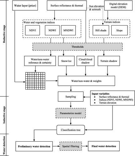
2.2.1. Deductive stage

The first stage of classification generates local reference data with varying levels of certainty. The pixels, identified as water by multispectral indices, were compared with a priori water pixels resampled from the 250-m-resolution MODIS water mask to the spatial resolution and extent of each Landsat image. The comparison results in four possible levels of certainty, through which weights were assigned to each reference datum (Table 2).

Table 2. Weighting of strata identified by spectral and terrain indices and by agreement with the MODIS water mask.

Data	Stratum	Agreement with MODIS water mask	Weight
Landsat indices	High certainty water	Agree	1.0
		Disagree	0.5
	Low certainty water	Agree	0.1
		Disagree	0.05
	Nonwater		0.1
	Snow/ice		0.3
Terrain indices	Terrain shadow		0.3

Topographic, spectral, and brightness temperature variables were first stratified into generic cover types: water, land, snow and ice, and cloud. A loose and a strict threshold – equaling −0.1 and 0.1 – were applied each to NDWI and MNDWI to distinguish water with low and high certainty. Terrain shadows were identified as pixels with hill-shade level <150 (on a scale from 0 to 255) and slope >20 degrees, as discussed in section 2.1.2.

Snow and ice show high reflectance in the visible and near-infrared bands and low reflectance in shortwave-infrared bands, leading to high MNDWI but low to moderate NDWI. A strict difference threshold (0.7) was used to reduce confusion of water with snow and ice, and a criterion of brightness temperature <1.5°C was also included to further improve the discrimination:

(4)

2.2.2. Inductive stage

A decision tree was then used to relate the certainty-weighted water reference data to reflectance and temperature estimates, multispectral indices, and elevation. A stratified random sample was drawn from each image by including pixels of each stratum (s) with probability of selection (p):

(5)

where N_s is the number of pixels to be drawn within the stratum in an image and N is the total number of pixels in that stratum in the image. A random value between 0.0 and 1.0 was generated for each pixel, and the pixel was selected for the sample if its random value was < p_s. N_s was set to 20,000 for each stratum. Weights, representing certainty of water identification within the strata, were set through extensive preliminary testing and were used to adjust the objective (i.e. purity) function maximized by the decision tree (Quinlan 1986). The confidence estimated for each pixel was recorded and saved as a separate spatial layer. Identified cloud/shadow and snow/ice pixels were also labeled in the data.

2.3. Post-classification filtering and compositing

Following classification, a 5-pixel majority within a 3-pixel-radius filter was applied to each pixel to remove high-frequency noise and to check pixels near the edge of identified water bodies in order to avoid dropping edge pixels with weak water signals. Each Landsat scene was processed independently, and overlapping pixels from multiple images were composited by selecting the result at each location with highest posterior (water/nonwater) probability. This ‘best-pixel’ compositing maximized classification certainty and filled gaps due to clouds and their shadows (Sexton, Song, Feng, et al. 2013; Kim et al. 2014).

Finally, inland water was distinguished from marine water by referring to the Global Database of Administrative areas (GADM) version 2 (http://www.gadm.org/). The GDAM vector layer was rasterized to the resolution and spatial extent of each Landsat scene. The identified water pixels located outside of administrative areas were labeled as ocean pixels and removed from the inland water layer.

2.4. Computation

The algorithm was implemented using C and Python programming languages. Open-source libraries, i.e. Geospatial Data Abstraction Library (http://www.gdal.org/), PROJ4 (http://trac.osgeo.org/proj/), NumPy (http://www.numpy.org/), SciPy (http://www.scipy.org/), and Matplotlib (http://matplotlib.org/) were used to enable application on both Linux and Windows platforms. The decision tree model was parameterized using C5.0, developed by RuleQuest Research (open-source single-thread version, http://www.rulequest.com/).

Multiple-processing techniques were applied in the high-performance computing cluster at GLCF (www.landcover.org).With 10 servers (16 cores and 64-GB memory each), the 8756 Landsat ETM+ images were processed within 24 hours. Results were stored in GeoTIFF format with embedded color scheme to facilitate viewing using image-viewer and Geographic Information System software.

2.5. Cross-comparison with previous global and national datasets

Because of the water dynamics and global coverage at 30-m, it is practically impossible to perform full validation of the dataset. However, cross-comparing the dataset with other water datasets produced for similar period would provide an assessment of the data quality.

2.5.1. Global assessment against the MODIS water mask

The resulting GLCF inland surface water dataset (GIW) was compared globally with the MODIS water mask (Carroll et al. 2009) to assess its consistency relative to the more established product. The 30-m-resolution Landsat data were reprojected to MODIS’ sinusoidal projection, aggregated to percent water within each 250-m-resolution MODIS pixel, and those Landsat pixels with percent water ≥50% were labeled as water. Although the GLS images were selected preferentially within the growing season, the acquisition dates vary from scene to scene, causing differences in water areas due to seasonal water changes. We therefore also investigated the differences between the MODIS and Landsat datasets in each scene. For this, the MODIS water mask was reprojected and resampled to the (30-m) resolution and extent of each Landsat image. Percentages of water within the scene were calculated for both datasets and compared graphically and numerically following Willmott (1982).

2.5.2. Assessment against national land-cover datasets

To assess accuracy relative to independent sources at native (30-m) resolution, GIW were compared with two 30-m-resolution, circa-2000 national land-cover products. User’s accuracy (UA), producer’s accuracy (PA), and overall accuracy (Foody 2002) were calculated to measure the differences among our estimates and those of the established Landsat-resolution datasets.

2.5.2.1. NLCD 2001

The 2001 National Land Cover Database (NLCD 2001) (Homer et al. 2004) was developed by USGS as the second generation of the Multi-Resolution Land Characterization (MRLC) 2001 to provide a 30-m-resolution land-cover map for contiguous United States. NLCD 2001 comprised 29 cover classes, including a class for open water. The dataset was based primarily on a decision-tree classification of circa-2001 Landsat satellite data and DEM-based topographic variables (Homer et al. 2004). Validated against expert human interpretation of high-resolution imagery, the reported accuracy of NLCD 2001 exceeds 80% for water (Wickham et al. 2013). The dataset was downloaded from the MRLC website (http://www.mrlc.gov/) in GeoTIFF format.

2.5.2.2. EOSD

The Canadian EOSD land-cover dataset was developed by the Canadian Forest Service and Canadian Space Agency. The EOSD dataset was produced using Landsat images acquired in circa-2000 (Wulder et al. 2003). The dataset covers the forested area of Canada, about half of the Canada landmass, and the nonforested northern portions and agricultural southern portions of the country were not mapped (Wulder et al. 2003). User’s and producer’s accuracies of water were >91% (Wulder et al. 2006).

3. Results

3.1. GIW, version 1.0

Figure 2 presents a global mosaic of the GIW, version 1.0. The data estimate 3,650,723 km² of inland surface water in circa-2000, nearly three quarters of which was located in North America (40.65%) and Asia (32.77%), followed by Europe (9.64%), Africa (8.47%), South America (6.91%), and Oceania (1.57%) (Table 3). Of the major biomes (Olson et al. 2001), boreal forests contained the largest portion of terrestrial surface water, with 25.03% of the global total. The nominal ‘inland water’ biome delineated by Olson et al. (2001) held 16.36% of the total. Tundra held 15.67%, and temperate broadleaf and mixed forests held 13.91%. The remaining ~30% was distributed among the other biomes (Table 3).

Figure 2. Global water data derived from the 8756 Landsat ETM+ images in the GLS 2000 dataset.

Note: The data were spatially aggregated from binary (water/nonwater) at 30-m-resolution to percent water at 0.1 degree resolution for display.

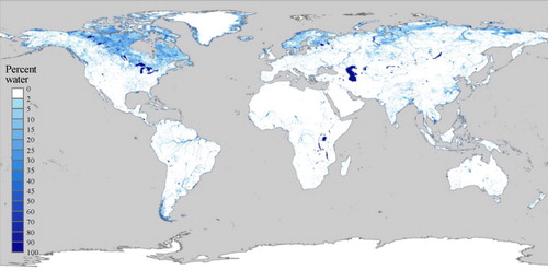
Table 3. Estimates of water areas for 6 continents and 16 major terrestrial biomes.

Regions	Regional area (km^2)	Water area (km^2)	Percent of global water
Continent
North America	23,956,255	1,474,229	40.65%
Asia	44,567,239	1,188,441	32.77%
Europe	9,769,792	349,433	9.64%
Africa	29,975,249	307,093	8.47%
South America	17,720,425	250,472	6.91%
Oceania	8,087,537	56,990	1.57%
Biome
Boreal forests/taiga	16,010,042	913,925	25.03%
Inland water	638,367	597,305	16.36%
Tundra	7,548,658	571,946	15.67%
Temperate broadleaf and mixed forests	12,756,218	507,774	13.91%
Tropical and subtropical moist broadleaf forests	19,796,794	287,850	7.88%
Deserts and xeric shrublands	27,933,025	157,039	4.30%
Temperate grasslands, savannas, and shrublands	9,615,946	155,112	4.25%
Tropical and subtropical grasslands, savannas, and shrublands	19,520,404	143,678	3.94%
Temperate conifer forests	4,296,433	69,496	1.90%
Montane grasslands and shrublands	5,191,805	69,290	1.90%
Flooded grasslands and savannas	1,093,123	54,512	1.49%
Tropical and subtropical dry broadleaf forests	3,794,229	49,734	1.36%
Mangroves	320,380	31,400	0.86%
Mediterranean forests, woodlands, and scrub	3,244,477	25,682	0.70%
Rock and ice	1,798,268	13,265	0.36%
Tropical and subtropical coniferous forests	643,218	2715	0.07%

Note: Biomes were taken from ‘Major Habitat Types’ of Olson et al. (2001).

3.2. Cross-comparison with previous global and national datasets

3.2.1. Global comparison to the MODIS water mask

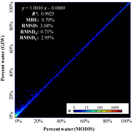
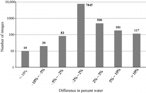
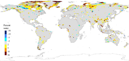
Correlation between GIW (v1.0) and the MODIS water mask was strongly linear (R ² > 0.99), with a slope of 1.001 and offset of −0.0069% cover (Figure 3). Mean Bias Error (MBE) was 0.70%, and RMSD was 3.04%, divided between smaller systematic errors (RMSD_S) of 0.71% and larger unsystematic (random) errors (RMSD_U) of 2.95%. Differences between the GIW and MODIS estimates were within ±2% of area in 7845 Landsat images (89.6% of the GLS 2000 dataset) (Figure 4). Significant differences (>±10%) were found in 127 images (1.5% of the GLS 2000), most of which were above 65°N (Figure 5) – these included areas on the coast of Greenland; Northern Qikiqtaaluk Region, Canada; and Arkhangelsk, Russia. Pixel-level comparison shows strong agreement between GIW and the MODIS water mask, with UA >99% and PA >90% (Table 4).

Table 4. Confusion matrix for pixel-level comparison between GIW and MODIS water mask.

	GIW
Reference dataset		Water (pixels)	Land (pixels)	PA (%)
MODIS water mask	Water (pixels)	1,842,316,302	193,344,155	90.50%
	Land (pixels)	14,508,334	4,707,419,000	99.69%
	UA (%)	99.22%	96.05%	96.92%

Figure 3. Comparison of percent-water area estimated by GIW and the MODIS water mask (Carroll et al. 2009) for the 8756 Landsat scenes.

Note: Correlation at the global scale was strongly linear, with R² > 0.99, slope ≈ 1, and offset ≈ 0.

Figure 4. Frequency distribution (log-scale) of scene-level difference between GIW and MODIS water mask (Carroll et al. 2009) estimates of percent-water area.

Figure 5. Spatial distribution of difference between GIW and MODIS water mask, calculated by subtracting the MODIS estimated percent water from the Landsat estimation for each Landsat image.

3.2.2. Comparison with national land-cover datasets

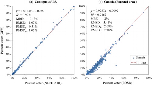
GIW showed strong agreement with U.S. NLCD 2001 and Canadian EOSD (Table 5), with user’s and overall accuracies (UA and PA) >95%. PA against NLCD 2001 was >95%, but was only 86.45% when compared with EOSD, suggesting comparatively weak sensitivity to water at high latitudes by GIW. Inland water area estimated by GIW was 405,258 km² over the contiguous United States and 995,083 km² over the forested area of Canada, lower than estimates of the national datasets by 0.8% and 9.8%, respectively.

Table 5. Confusion matrix for pixel-level comparison between GIW and two national land-cover datasets.

	GIW
Reference dataset		Water (km^2)	Land (km^2)	Reference estimated area (km^2)	PA (%)
EOSD	Water (km^2)	953,789	149,465	1,103,254	86.45%
	Land (km^2)	41,294	2,816,275	2,857,569	98.55%
	Landsat estimated area (km^2)	995,083	2,965,740	3,960,823
	UA (%)	95.85%	94.96%		95.18%
NLCD 2001	Water (km^2)	389,487	19,288	408,775	95.28%
	Land (km^2)	15,771	6,411,536	6,427,307	99.75%
	Landsat estimation area (km^2)	405,258	6,430,824
	UA (%)	96.11%	99.70%		99.49%

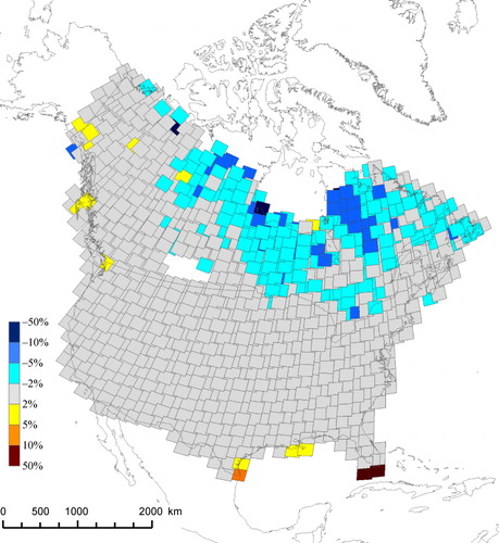
Aggregated to the resolution of Landsat scenes, the RMSD of percent-water estimates from GIW relative to that of NLCD 2001 and of EOSD percent-water layers were 1.07% and 3.41%, respectively (Figure 6). RMSD_S (0.31%) was lower than RMSD_U (1.02%) when compared with NLCD 2001, indicating the differences between the two estimations were also mainly due to random errors. Differences were largest in floodplains along the Mississippi delta and near coasts, the latter due largely to tidal differences between observations (Figure 7). Correlation between the two sets of estimates was very strong, with slope = 1.0133, offset = −0.0025, and R ² = 0.9971. Compared against EOSD, RMSD_S and RMSD_U were both >2% and MBE was −2%, suggesting slight underestimation of water cover in Canada by GIW. Correlation of GIW with EOSD estimates was lower than with those of NLCD 2001 yet still very high, with slope = 0.9257, offset = −0.0097, and R ² = 0.9971. Outliers were mainly due to ice and snow overlying water, such as in areas surrounding Hudson Bay and Northern Ungava Peninsula in Canada.

Figure 6. Comparison of percent water estimated by GIW and regional land-cover datasets over (a) the contiguous United States (NLCD 2001) and (b) the forested area of Canada (EOSD) at the resolution of Landsat scenes.

Figure 7. Spatial distribution of scene-level difference between percent water estimated by GIW and regional land-cover datasets over the contiguous United States and Canada, calculated by subtracting the MODIS estimate from the GIW estimate of percent water for each Landsat scene.

4. Discussion

4.1. Automated high-resolution inland water data

GIW depicts at high (30-m) resolution the circa-2000 growing season coverage of Earth’s inland fresh and saline water bodies larger than 0.5 ha. Relative to global and national datasets, its errors appear to be small and predominantly unbiased – except in northern latitudes where water was temporarily covered by snow and ice. The data provide a more detailed depiction of inland water bodies than existing coarse-resolution global masks and a more globally consistent representation than is afforded by national data products. Technically, the dataset demonstrates the ability to detect water with minimal human supervision. The algorithm requires only the definition of weights to refine prior estimates – thus enabling the consistent detection of inland surface water over large areas.

Estimation of global water area based on high-resolution satellite imagery has increased in recent years. Although these new datasets are not yet publicly available for pixel-level comparison, comparison of their global-area estimates to ours reveals a mixed consensus. Using a manually edited, supervised classification approach (Liao et al. 2014), the National Remote Sensing Center of China (NRSCC) identified 3,676,700 km² of global inland water in 2010–2011 (NRSCC 2012). The NRSCC and GIW estimates differ by 25,977 km² (0.7% of global inland water area), despite changes from the GLS2000 epoch to the 2010–2011 span of the NRSCC record. In contrast, Verpoorter et al. (2014) recently estimated 5 × 10⁶ km² of inland water area globally. The NRSCC and our results suggest that the Verpoorter et al. (2014) estimate is likely an overestimate – especially since their comparatively large estimate focused on lakes but excluded rivers.

4.2. Combining terrain and water indices

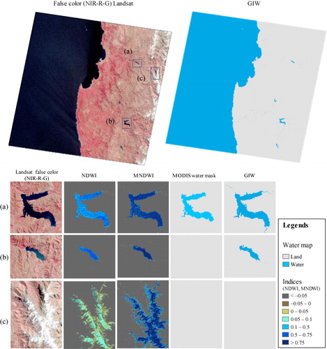
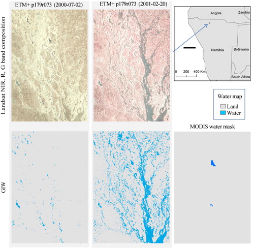
Figure 8 presents a comparison of multispectral water indices, the MODIS water mask, and GIW in a region of extreme topographic and hydrological variability. The two water indices, NDWI and MNDWI, are highly sensitive to water but poorly discriminate liquid water from frozen water (snow and ice) and terrain shadows. Complementarily, the MODIS water mask discriminates water from snow and ice, but frequently omits small water bodies. GIW combines these various sources of information to produce a more accurate representation of small and large water bodies while maintaining the distinction between liquid and frozen water.

Figure 8. Comparison of water indices (NDWI, MNDWI) and GIW from ETM+ image acquired on 20 September 2002, at WRS-2 p001r081 located in Coquimbo Region, Chile.

4.3. Remaining issues

Although GIW exhibits UA >95% relative to the national datasets, its PA was substantially lower (85%). This dominance of systematic (omission) errors suggests a difference in sensitivity between GIW and the national datasets. Whereas the national datasets each were based on multiple images in each location, the GLS Landsat dataset was based on a single image selected with preference for the growing season (Gutman et al. 2008). Inland water in many regions is a highly seasonal phenomenon. With one Landsat image for each location, GIW provides a static representation of inland water area at the time of image acquisition. Hence, although the water observed by the GLS acquisition would be expected to avoid low water levels in the dry season of arid and semiarid regions, this could lead to failure to represent intra-annual water fluctuations in regions of high seasonal variability. Also, visual inspection revealed that narrow rivers and streams were often not or only partially detected. When the width of rivers was less or close to the Landsat resolution (30 m), the water signal became weak because of mixing with surrounding land. Due to the limitation of optical sensors, GIW was able to identify exposed water, with likely underestimation in flooded forests, snow/ice-covered areas, and beneath residual clouds. A small amount of offshore pixels were included erroneously over coastlines with complex topography, such as the southern tip of South America and Greenland coast, as a result of imprecision in GADM. Other factors – such as water depth, suspended sediment load, and presence of emergent or floating vegetation – also hindered discrimination locally. In addition to terrain shadow, shadow of tall buildings can also be identified with the 30-m-resolution DEM (Jacobsen and Passini 2010; Tachikawa et al. 2011). The uncaught shadows of short buildings are likely to be isolated pixels and were expected to be excluded by the 5-pixel filter rule.

4.3.1. Seasonality and extreme events

Inland water bodies change over time, yet single (e.g. Landsat) images provide only snapshots of their dynamics. Intra-annual variation likely led to inconsistencies between GIW estimates based on single images versus national datasets based on multiple images. The GLS images were preferentially acquired during the growing season, but their actual acquisition dates range across the entire year, depending on availability (Kim et al. 2011). These dates were not identical to those of the Landsat images used for producing the NLCD and EOSD. Figure 9 presents an example showing inconsistencies in the detection of water bodies due to seasonal water changes. Due to the preferences of the GLS image selection, GIW delineates water primarily in the growing season of each region. However, the water bodies observed were also affected by extreme weather events such as flooding, drought, and late-season snow and ice cover. Corroborating other recent studies mapping various land-cover types (Sexton, Song, Huang, et al. 2013; Sexton, Urban, et al. 2013), temporal compositing with additional Landsat imagery will likely provide a more comprehensive estimation of global water area and changes.

Figure 9. Water body difference due to seasonal variation in Natukanaoka Pan, Nambia.

Note: Because of the large water fluctuation between wet and dry seasons, the two Landsat images (i.e. ETM+ acquired on 2 July 2000 at WRS-2 p180r072 and 20 February 2001 at p179r073) happened to catch the difference. To show the effect of resolution, the MODIS water mask is also presented for comparison.

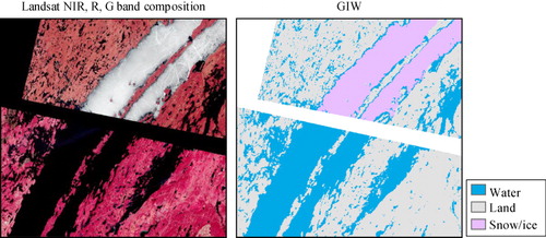
Intermittent snow and ice contributed to additional error. Optical wavelengths do not penetrate snow and ice overlaying water bodies, and so water cover was underestimated in images where snow and ice temporarily obscured water. Because high latitudes have shorter summers, there was higher chance for Landsat images to observe water bodies in these regions when covered with snow and ice. Figure 10 shows the distribution of water captured by GIW near Lake Mistassini, Canada. The bottom part of the scene was acquired on 28 August 2002, which shows a clear view of the lakes. The lakes were covered with ice when the upper Landsat ETM+ image was acquired on 14 May 2001. Hence, GIW underestimated water area for the scene, causing the lower outlier Figure 6. The seasonal weather conditions largely caused the inconsistency between the water areas detected from the Landsat images. As with problems related to seasonality of (liquid) water, issues due to seasonal snow and ice cover over water can be minimized by compositing greater volumes of imagery within a year.

Figure 10. Water body derived for the central part of Lake Mistassini, Canada.

Note: The Landsat ETM+ acquired on 28 August 2002, at p016r025 showing a clear image of the water bodies, which were covered with ice in the ETM+ acquired on 14 May 2001, at p015r024.

4.3.2. Residual clouds

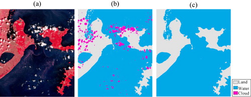
Although most clouds were removed before water detection, residual undetected clouds contributed additional classification errors. Also, removal of pixels imparts uncertainty to regional estimation of water coverage. Given that erroneous clouds are typically associated with low certainty values, incorporating additional images into composites will likely remove errors due to residual clouds. Figure 11 provides an example of adding extra Landsat images to provide a cloud-free water body map for Uganda. The GLS and extra Landsat images were processed individually, and their water estimates were overlaid and composited using the best-pixel rule. Although the two images were each contaminated by residual clouds, the composited result was cloud-free.

Figure 11. Filling cloud-contaminated observations with additional Landsat images.

Note: (a) The false-color band combination (NIR-R-G) of ETM+ image from GLS 2000 acquired on 27 November 2001, at WRS-2 p171r060. (b) The water data derived from the Landsat scene. (c) Updated cloud-free water data using the best pixel compositing rule (see section 2.3), and the extra image was acquired on 9 July 2002, at the same WRS-2 tile.

5. Conclusions

We developed an automated method for mapping inland surface water bodies by combining coarse-resolution, global estimates of water cover with high-resolution estimates of surface reflectance and topographic indices. The method has been implemented with open-source libraries to facilitate processing large amounts of Landsat images on high-performance computing machines. With the support of the computing environment at GLCF, the method has been applied to the roughly 9000 Landsat scenes of the GLS 2000 data collection to produce a global, 30-m-resolution inland surface water body dataset (GIW) for circa-2000. The GIW version-1.0 is publicly available at the GLCF website (http://www.landcover.org).

GIW provides an estimation of regional and global inland water area for circa-2000 at higher resolution than the prior global MODIS water mask. From the dataset, 3,650,723 km² of inland water were identified, around three quarters of which were in North America and Asia. Boreal forests and tundra hold the largest portion of inland water, about 40% of the global total.

GIW exhibits strong linear correlation with both the MODIS dataset as well as 30-m-resolution datasets over the United States and Canada. Residual errors were due primarily to the seasonality of water cover, snow and ice, and residual clouds. Most errors can be removed by compositing larger numbers of Landsat images per scene.

The sub-hectare resolution of the Landsat sensors provides a more detailed global observation of inland surface water than previously possible. The automated method we present here detects water in Landsat images with minimal human input, using a two-stage procedure to leverage and refine prior information. Based on the long-term record provided by the newly opened USGS Landsat archive, our automated method can facilitate retrieval of global inland surface water and its dynamics at high-resolution spanning the past four decades. The method can also promote water monitoring with data acquired from other satellites, especially those with spectral bands similar to those of the Landsat sensors.

Acknowledgements

All data handling and processing were performed at the GLCF. The authors greatly thank Dr. Chengquan Huang for the cloud identification and masking code. The authors also thank their colleagues Xiao-Peng Song, Dan-Xia Song, Do-Hyung Kim, and Kathrine Collins for their constructive comments.

Disclosure statement

No potential conflict of interest was reported by the authors.

Additional information

Funding

This research was supported by the following NASA programs: Making Earth System Data Records for Use in Research Environments (MEaSUREs) [NNX08AP33A], Land-Cover and Land-Use Change (LCLUC) [NNX08AN72G], and Advancing Collaborative Connections for Earth System Science (ACCESS) [NNX12AH18A].

References

- Carroll, M. L., J. R. G. Townshend, C. M. DiMiceli, T. Loboda, and R. A. Sohlberg. 2011. “Shrinking Lakes of the Arctic: Spatial Relationships and Trajectory of Change.” Geophysical Research Letters 38 (20406): 1–5. doi:10.1029/2011GL049427.
- Carroll, M. L., J. R. Townshend, C. M. DiMiceli, P. Noojipady, and R. A. Sohlberg. 2009. “A New Global Raster Water Mask at 250 M Resolution.” International Journal of Digital Earth 2 (4): 291–308. doi:10.1080/17538940902951401.
- Cole, J. J., Y. T. Prairie, N. F. Caraco, W. H. McDowell, L. J. Tranvik, R. G. Striegl, C. M. Duarte, et al. 2007. “Plumbing the Global Carbon Cycle: Integrating Inland Waters into the Terrestrial Carbon Budget.” Ecosystems 10 (1): 172–185. doi:10.1007/s10021-006-9013-8.
- Craglia, M., K. de Bie, D. Jackson, M. Pesaresi, G. Remetey-Fülöpp, C. Wang, A. Annoni, et al. 2012. “Digital Earth 2020: Towards the Vision for the next Decade.” International Journal of Digital Earth 5 (1): 4–21. doi:10.1080/17538947.2011.638500.
- Famiglietti, J. S., and M. Rodell. 2013. “Water in the Balance.” Science 340: 1300–1301. doi:10.1126/science.1236460.
- Farr, T. G., P. A. Rosen, E. Caro, R. Crippen, R. Duren, S. Hensley, M. Kobrick, et al. 2007. “The Shuttle Radar Topography Mission.” Reviews of Geophysics 45 (2): 1–33. doi:10.1029/2005RG000183.
- Feng, M., C. Huang, S. Channan, E. F. Vermote, J. G. Masek, and J. R. Townshend. 2012. “Quality Assessment of Landsat Surface Reflectance Products Using MODIS Data.” Computers & Geosciences 38 (1): 9–22. doi:10.1016/j.cageo.2011.04.011.
- Feng, M., J. O. Sexton, C. Huang, J. G. Masek, E. F. Vermote, F. Gao, R. Narasimhan, et al. 2013. “Global Surface Reflectance Products from Landsat: Assessment Using Coincident MODIS Observations.” Remote Sensing of Environment 134: 276–293. doi:10.1016/j.rse.2013.02.031.
- Feyisa, G. L., H. Meilby, R. Fensholt, and S. R. Proud. 2014. “Automated Water Extraction Index: A New Technique for Surface Water Mapping Using Landsat Imagery.” Remote Sensing of Environment 140: 23–35. doi:10.1016/j.rse.2013.08.029.
- Foody, G. M. 2002. “Status of Land Cover Classification Accuracy Assessment.” Remote Sensing of Environment 80 (1): 185–201. doi:10.1016/S0034-4257(01)00295-4.
- Franks, S., J. Masek, R. Headley, J. Gasch, S. Covington, and T. Arvidson. 2009. “Large Area Scene Selection Interface (LASSI): Methodology of Selecting Landsat Imagery for the Global Land Survey 2005.” Photogrammetric Engineering and Remote Sensing 75: 1287–1296. doi:10.14358/PERS.75.11.1287.
- Gao, F., J. Masek, M. Schwaller, and F. Hall. 2006. “On the Blending of the Landsat and MODIS Surface Reflectance: Predicting Daily Landsat Surface Reflectance.” IEEE Transactions on Geoscience and Remote Sensing 44: 2207–2218. doi:10.1109/TGRS.2006.872081.
- Gutman, G., R. Byrnes, J. Masek, S. Covington, C. Justice, S. Franks, and R. Headley. 2008. “Towards Monitoring Land-Cover and Land-Use Changes at a Global Scale: The Global Land Survey 2005.” Photogrammetric Engineering & Remote Sensing 74 (1): 6–10.
- Homer, C., C. Huang, L. Yang, B. Wylie, and M. Coan. 2004. “Development of a 2001 National Land-Cover Database for the United States.” Photogrammetric Engineering & Remote Sensing 70: 829–840. doi:10.14358/PERS.70.7.829.
- Horn, B. K. P. 1981. “Hill Shading and the Reflectance Map.” Proceedings of the IEEE 69 (1): 14–47. doi:10.1109/PROC.1981.11918.
- Huang, C., N. Thomas, S. N. Goward, J. G. Masek, Z. Zhu, J. R. G. Townshend, and J. E. Vogelmann. 2010. “Automated Masking of Cloud and Cloud Shadow for Forest Change Analysis Using Landsat Images.” International Journal of Remote Sensing 31: 5449–5464. doi:10.1080/01431160903369642.
- Jacobsen, K., and R. Passini. 2010. “Analysis of ASTER GDEM Elevation Models.” In The 2010 Canadian Geomatics Conference and Symposium of Commission I, ISPRS Convergence in Geomatics – Shaping Canada's Competitive Landscape. Vol. XXXVIII, part 1. Calgary, Alberta, Canada, June 15–18. http://www.isprs.org/proceedings/xxxviii/part1/09/09_03_Paper_103.pdf.
- Ji, Lei, L. Zhang, and B. Wylie. 2009. “Analysis of Dynamic Thresholds for the Normalized Difference Water Index.” Photogrammetric Engineering & Remote Sensing 75: 1307–1317. doi:10.14358/PERS.75.11.1307.
- Jiang, H., M. Feng, Y. Zhu, N. Lu, J. Huang, and T. Xiao. 2014. “An Automated Method for Extracting Rivers and Lakes from Landsat Imagery.” Remote Sensing 6: 5067–5089. doi:10.3390/rs6065067.
- Kaufman, Y. J., and D. Tanré. 1996. “Strategy for Direct and Indirect Methods for Correcting the Aerosol Effect on Remote Sensing: >From AVHRR to EOS-MODIS.” Remote Sensing of Environment 55 (1): 65–79. doi:10.1016/0034-4257(95)00193-X
- Kim, D.-H., R. Narashiman, J. O. Sexton, C. Huang, and J. R. Townshend. 2011. “A Methodology to Select Phenologically Suitable Landsat Scenes for Forest Change Detection.” In 2011 IEEE International Geoscience and Remote Sensing Symposium (IGARSS), 2613–2616. Vancouver, Canada, July 24–29. doi:10.1109/IGARSS.2011.6049738.
- Kim, D.-H., J. O. Sexton, P. Noojipady, C. Huang, A. Anand, S. Channan, M. Feng, and J. R. Townshend. 2014. “Global, Landsat-Based Forest-Cover Change from 1990 to 2000.” Remote Sensing of Environment 155: 178–193. doi:10.1016/j.rse.2014.08.017.
- Liao, A., L. Chen, J. Chen, C. He, X. Cao, J. Chen, S. Peng, et al. 2014. “High-Resolution Remote Sensing Mapping of Global Land Water.” Science China Earth Sciences 57: 2305–2316. doi:10.1007/s11430-014-4918-0.
- Masek, J. G., E. F. Vermote, N. E. Saleous, R. Wolfe, F.G. Hall, K.F. Huemmrich, F. Gao, et al. 2006. “A Landsat Surface Reflectance Dataset for North America, 1990–2000.” IEEE Geoscience and Remote Sensing Letters 3 (1): 68–72. doi:10.1109/LGRS.2005.857030.
- Maxwell, S. K., G. L. Schmidt, and J. C. Storey. 2007. “A multi‐scale segmentation approach to filling gaps in Landsat ETM+ SLC‐off images”. International Journal of Remote Sensing 28: 5339–5356. doi:10.1080/01431160601034902.
- McFeeters, S. K. 1996. “The Use of the Normalized Difference Water Index (NDWI) in the Delineation of Open Water Features.” International Journal of Remote Sensing 17: 1425–1432. doi:10.1080/01431169608948714.
- NRSCC. 2012. “Global Land Surface Water 2010 and Dynamic Changes of Sample Lakes 2001-2011”. Beijing, China: National Remote Sensing Center of China (NRSCC). http://www.chinageoss.org/gee/2012/index_en_sy.html.
- Olson, D. M., E. Dinerstein, E. D. Wikramanayake, N. D. Burgess, G. V. N. Powell, E. C. Underwood, J. A. D’Amico, et al. 2001. “Terrestrial Ecoregions of the World: A New Map of Life on Earth.” BioScience 51: 933–938. doi:10.1641/0006-3568(2001)051[0933:TEOTWA]2.0.CO;2.
- Quinlan, J. R. 1986. “Induction of Decision Trees.” Machine Learning 1 (1): 81–106.
- Rabus, B., M. Eineder, A. Roth, and R. Bamler. 2003. “The Shuttle Radar Topography Mission—A New Class of Digital Elevation Models Acquired by Spaceborne Radar.” ISPRS Journal of Photogrammetry and Remote Sensing 57 (4): 241–262. doi:10.1016/S0924-2716(02)00124-7.
- Sexton, J. O., X.-P. Song, M. Feng, P. Noojipady, A. Anand, C. Huang, D.-H. Kim, et al. 2013. “Global, 30-M Resolution Continuous Fields of Tree Cover: Landsat-Based Rescaling of MODIS Vegetation Continuous Fields with Lidar-Based Estimates of Error.” International Journal of Digital Earth 6: 427–448. doi:10.1080/17538947.2013.786146.
- Sexton, J. O., X.-P. Song, C. Huang, S. Channan, M. E. Baker, and J. R. Townshend. 2013. “Urban Growth of the Washington, D.C.–Baltimore, MD Metropolitan Region from 1984 to 2010 by Annual, Landsat-Based Estimates of Impervious Cover.” Remote Sensing of Environment 129: 42–53. doi:10.1016/j.rse.2012.10.025.
- Sexton, J. O., D. L. Urban, M. J. Donohue, and C. Song. 2013. “Long-Term Land Cover Dynamics by Multi-Temporal Classification across the Landsat-5 Record.” Remote Sensing of Environment 128: 246–258. doi:10.1016/j.rse.2012.10.010.
- Shevyrnogov, A. P., A. V. Kartushinsky, and G. S. Vysotskaya. 2002. “Application of Satellite Data for Investigation of Dynamic Processes in Inland Water Bodies: Lake Shira (Khakasia, Siberia), A Case Study.” Aquatic Ecology 36 (2): 153–164. doi:10.1023/A:1015658927683.
- Sun, F., W. Sun, J. Chen, and P. Gong. 2012. “Comparison and Improvement of Methods for Identifying Waterbodies in Remotely Sensed Imagery.” International Journal of Remote Sensing 33: 6854–6875. doi:10.1080/01431161.2012.692829.
- Tachikawa, T., M. Kaku, A. Iwasaki, D. Gesch, M. Oimoen, Z. Zhang, J. Danielson et al. 2011. “ASTER Global Digital Elevation Model Version 2 – Summary of Validation Results.” Accessed June 17, 2014. http://www.jspacesystems.or.jp/ersdac/GDEM/ver2Validation/Summary_GDEM2_validation_report_final.pdf.
- Townshend, J. R. G., and C. O. Justice. 1988. “Selecting the Spatial Resolution of Satellite Sensors Required for Global Monitoring of Land Transformations”. International Journal of Remote Sensing 9 (2): 187–236. doi:10.1080/01431168808954847.
- Townshend, J. R., J. G. Masek, C. Huang, E. F. Vermote, F. Gao, S. Channan, J. O. Sexton, et al. 2012. “Global Characterization and Monitoring of Forest Cover Using Landsat Data: Opportunities and Challenges.” International Journal of Digital Earth 5 (5): 373–397. doi:10.1080/17538947.2012.713190.
- Tucker, C. J., D. M. Grant, and J. D. Dykstra. 2004. “NASA’s Global Orthorectified Landsat Data Set.” Photogrammetric Engineering and Remote Sensing 70 (3): 313–322. doi:10.14358/PERS.70.3.313.
- Tucker, C., J. Pinzon, M. Brown, D. Slayback, E. Pak, R. Mahoney, E. Vermote, and N. E. Saleous. 2005. “An Extended AVHRR 8-km NDVI Dataset Compatible with MODIS and SPOT Vegetation NDVI Data.” International Journal of Remote Sensing 26: 4485–4498. doi:10.1080/01431160500168686.
- USGS. 2012. “SRTM Water Body Dataset.” Accessed June 17, 2014. https://lta.cr.usgs.gov/srtm_water_body_dataset.
- Verpoorter, C., T. Kutser, and L. Tranvik. 2012. “Automated Mapping of Water Bodies Using Landsat Multispectral Data.” Limnology and Oceanography: Methods 10: 1037–1050. doi:10.4319/lom.2012.10.1037.
- Verpoorter, C., T. Kutser, David a. Seekell, and L. J. Tranvik. 2014. “A Global Inventory of Lakes Based on High-Resolution Satellite Imagery.” Geophysical Research Letters 41 (18): 6396–6402. doi:10.1002/2014GL060641.
- Wickham, J. D., S. V. Stehman, L. Gass, J. Dewitz, J. A. Fry, and T. G. Wade. 2013. “Accuracy Assessment of NLCD 2006 Land Cover and Impervious Surface.” Remote Sensing of Environment 130: 294–304. doi:10.1016/j.rse.2012.12.001.
- Willmott, C. J. 1982. “Some Comments on the Evaluation of Model Performance.” Bulletin of the American Meteorological Society 63: 1309–1313. doi:10.1175/1520-0477(1982)063<1309:SCOTEO>2.0.CO;2.
- Wulder, M. A., J. A. Dechka, M. A. Gillis, J. E. Luther, R. J. Hall, A. Beaudoin, and S. E. Franklin. 2003. “Operational Mapping of the Land Cover of the Forested Area of Canada with Landsat Data: EOSD Land Cover Program.” The Forestry Chronicle 79 (6): 1075–1083. doi:10.5558/tfc791075-6.
- Wulder, M. A, J. C. White, J. E. Luther, G. Strickland, T. K. Remmel, and S. W. Mitchell. 2006. “Use of Vector Polygons for the Accuracy Assessment of Pixel-Based Land Cover Maps.” Canadian Journal of Remote Sensing 32 (3): 268–279. doi:10.5589/m06-023.
- Xu, H. 2006. “Modification of Normalised Difference Water Index (NDWI) to Enhance Open Water Features in Remotely Sensed Imagery.” International Journal of Remote Sensing 27: 3025–3033. doi:10.1080/01431160600589179.