Channeling the water data deluge: a system for flexible integration and analysis of hydrologic data

Abstract

The hydrologic cycle and understanding the relationship between rainfall and runoff is an important component of earth system science, sustainable development, and natural disasters caused by floods. With this in mind, the integration of digital earth data for hydrologic sciences is an important area of research. Currently, it takes a tremendous amount of effort to perform hydrologic analysis at a large scale because the data to support such analyses are not available on a single system in an integrated format that can be easily manipulated. Furthermore, the state-of-the-art in hydrologic data integration typically uses a rigid relational database making it difficult to redesign the data model to incorporate new data types. The HydroCloud system incorporates a flexible document data model to integrate precipitation and stream flow data across spatial and temporal dimensions for large-scale hydrologic analyses. In this paper, a document database schema is presented to store the integrated data-set along with analysis tools such as web services for data access and a web interface for exploratory data analysis. The utility of the system is demonstrated based on a scientific workflow that uses the system for both exploratory data analysis and statistical hypothesis testing.

Keywords:

• hydrology
• data integration
• cloud-based systems
• NoSQL
• NEXRAD precipitation
• stream flow

1. Introduction

The hydrologic cycle and its impact on Earth systems is an active area of digital earth research. Two components of the hydrologic cycle, rainfall and stream flow, characterize what is known as the watershed response. This relationship is of particular interest to scientists due to its critical role in flooding. Large sensor networks and satellite systems have been deployed in order to better understand, predict, and mitigate future natural disasters from flooding and heavy rainfall. The volumes of data gathered in support of this work require new advances in digital earth technology to integrate disparate sources of hydrologic data.

The most basic way to analyze watershed response requires the integration of rainfall and stream flow data. More complicated analyses also require land cover and topography data, requiring the integration of numerous spatial and temporal data types. Much of this data is collected by Federal agencies in the USA who have made their data publicly available over the Internet. Despite these efforts, many of these hydrologic data products have not been used to their full potential, and are not used in conjunction with one another. For example, there has yet to be a system that effectively integrates precipitation data with stream flow to perform a simple rainfall–runoff analysis. In part, this is because the datasets are large and are stored in different locations, in different formats, by different agencies.

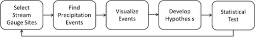
Our research is motivated by a scientific workflow that involves the exploratory analysis of hydrologic data, as presented in Figure 1. The first step in the workflow is to be able to explore an integrated set of hydrologic data to select stream gauge sites of interest. In this exploratory phase, the hydrologist would like to select stream gauge sites based on criteria such as drainage area, percent impervious surface (a measure of urbanization), and physiographic province. These criteria will likely relate to a research question such as: ‘how does the amount of impervious surface in a watershed affect runoff from storm events?’ Once the hydrologist generates a set of candidate sites, the next step is to find interesting precipitation events to evaluate. This will require a time series visualization that allows the hydrologist to easily plot precipitation and stream flow on the same x-axis. Once the events are found, a more detailed visualization may be needed to determine whether interesting relationships exist. Finally, these relationships can be summarized with a hypothesis that is evaluated against a statistical test.

Figure 1. Workflow for exploratory analysis of hydrologic data.

In order to make this scientific workflow a reality, a number of datasets have to be integrated. At the core of this analysis is the estimation of precipitation and stream flow. While stream flow data can be readily obtained using the USGS National Water Information System (NWIS), the estimation of precipitation is often a more difficult process. The most common method of estimation uses a network of rain gauges that are either within or proximal to a watershed. In most cases, the availability of quality rain gauge data is sparse, resulting in only one or two locations where precipitation is measured that may or may not be within the watershed in question. Recently, NEXRAD Radar has shown great potential for estimating precipitation at a much higher spatial resolution than that of most rain gauge networks (Krajewski et al. 2011). However, much of the focus thus far has been on the development of algorithms to convert NEXRAD reflectance to precipitation estimates. This problem has been worked on at a small scale in (McGuire and Sanderson 2010) using a web interface and relational database to serve averaged NEXRAD rainfall data. However, performance was limited where queries over a large number of points were prohibitively time-consuming.

The work presented in this paper is based on the HydroCloud system (McGuire, Roberge, and Lian 2014). The system integrates stream flow data from the USGS NWIS system with NOAA Stage IV NEXRAD rainfall data to provide tools for the analysis of the relationship between rainfall and runoff for a large number of watersheds. This work offers a number of novel contributions including (1) the use of a NoSQL document database for flexible integration of hydrologic data, (2) the design and development of extraction, transformation, and loading tools to harvest and integrate data from a variety of external sources, (3) the use of RESTful web services to provide access to the integrated data-set as well as a data delivery endpoint for a light-weight interface for exploring the integrated data-set, and (4) the utility of the HydroCloud system demonstrated in a real-world hydrologic analysis scenario. The paper is organized as follows: Section 2 presents existing literature that is related to this work, Section 3 presents the design of the HydroCloud system, Section 4 demonstrates the use of the HydroCloud system in the analysis of watershed response to storm events, and Section 6 discusses some future directions for this research.

2. Related work

The field of hydroclimatology seeks to discover linkages between atmospheric physics and the less well-understood processes of precipitation, runoff, and stream discharge. A number of database systems have been designed to integrate hydrologic data for this purpose. Previous work towards this goal includes the ArcHydro data model for Geographic Information Systems (GIS) analysis (Maidment 2002). The Consortium of Universities for the Advancement of Hydrologic Sciences has developed a Hydrologic Information System consisting of web services and analysis tools that allow users to access a variety of publicly available datasets (Maidment 2006; Goodall et al. 2008). One of the key components of this system is the Observations Data Model which is a relational database designed to store environmental observations (Horsburgh et al. 2009). Scientists have used these tools and data structures to model water quality (Ator, Brakebill, and Blomquist 2011) and to investigate connections between global processes and regional precipitation patterns (Svoma and Balling 2010).

Cloud-based data warehouses such as Hive have been shown to support data on the petabyte scale (Thusoo et al. 2010) and it is possible to conduct aggregation queries using the MapReduce framework (Brezany et al. 2011; Cao et al. 2011). The use of cloud architectures in geospatial science has been identified as an emerging technology that will extend cloud computing beyond its current technological boundaries (Yang et al. 2011). Recently, there has been some research on processing spatial queries using the MapReduce framework (Akdogan et al. 2010) and a grid-based architecture has been implemented on Amazon EC2 cloud storage to perform hydrologic simulation (Chiang et al. 2011). Most recently, a cloud-based architecture built on Hadoop has shown to be effective in querying spatial dimensions of scientific datasets (Aji and Wang 2012) and medical imaging (Aji, Wang, and Saltz 2012). Document databases such as MongoDB have shown to be very effective in the distributed management of spatial data (Han et al. 2013) and geoanalytic frameworks (Heard 2011). Finally, most related to the proposed work, a cloud architecture has also proven to be effective for visual analytics of climate data (Lu et al. 2011).

The HydroCloud system uses a document database to store and integrate hydrologic data (McGuire, Roberge, and Lian 2014). In this research, we utilize the HydroCloud system to perform an analysis of rainfall and runoff on a number of large watershed in Maryland, USA. We also extend the HydroCloud system to include a more robust database and extended Extraction, transformation and loading (ETL) workflows. This system can be implemented using cloud technology and scale out on a multi-node system. Another contribution that we make in this paper is the near-real time and scalable integration of gridded precipitation and stream flow data at watershed scale. To the authors’ knowledge, large-scale integration of NEXRAD precipitation data has never been done for this purpose. Furthermore, we use an extensible RESTful approach to data access and demonstrate the efficacy of our approach with a light-weight visualization interface designed for the exploration of rainfall and runoff data on a mobile web platform.

3. The HydroCloud system

The HydroCloud system integrates hydrologic data from a number of different sources, transforms them into documents, and stores them in a document database using MongoDB as the platform. The database is accessed through a number of web services through both a web client and tools developed for visualization and statistical analysis of hydrologic data. The architecture for the HydroCloud system is shown in Figure 2.

Figure 2. Overview of HydroCloud system architecture.

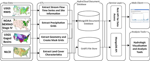
Data for the HydroCloud System comes from the USGS NWIS stream gauge database, NOAA Stage IV NEXRAD precipitation data, GIS layers for the USGS NWIS site watersheds, and the National Land Cover Database (NLCD). These datasets are automatically downloaded via collectors designed to extract data from web service protocols for NWIS data and ftp for the NWS rain gauges and NOAA Stage IV NEXRAD data. The collectors are responsible for ETL functions to transform data from their published formats to BSON documents to be stored in the document-oriented data warehouse based on MongoDB. Access to the HydroCloud data warehouse is provided through RESTful web services. The use of a web service API allows the web client to be developed in a modular fashion. Also, it allows other developers to access the HydroCloud system to create their own mash-ups and clients.

This paper presents the design of the HydroCloud data warehouse and focuses on the use of the HydroCloud system to support exploratory hydrologic analysis such at that shown in Figure 1. This section is organized as follows: Section 3.1 presents the datasets that are used in the HydroCloud system, Section 3.2 describes the document-oriented database model, Section 3.3 describes the ETL processes needed to build and continually update the HydroCloud database, Section 3.4 describes methods used to query the database, and Section 3.5 describes the web services interface as well as the associated web mapping and graphing interfaces that were developed to facilitate exploratory hydrologic analysis.

3.1. Datasets

The HydroCloud system integrates a number of datasets needed for hydrologic analysis. This includes stream flow data for all currently active gauges in the USGS NWIS system. The NWIS data was automatically ingested into the system using the NWIS Water Web Services (United States Geological Survey 2014) where a program was developed to automatically get data through a REST interface and transform the data to be loaded into the document database. The volume of data from the NWIS web services is about 200 kb per site per day. Given approximately 9000 active stream gauges in the USA, this could potentially result in easily over 1 GB of data per day. Precipitation data was collected from the NOAA National Stage IV Multisensor Mosaicked IPE Product (Lin and Mitchell 2005). This gridded precipitation data for the entire continental USA is created from a combination of NEXRAD 15 minute precipitation fields mosaicked and verified by a network of rain gauges. The Stage IV precipitation data is available at a temporal resolution of 1 hour. The volume of the Stage IV precipitation data is approximately 1 MB per grid resulting in approximately 24 MB per day. The Stage IV precipitation grids were masked using the USGS catchment boundaries for gauged watersheds (United States Geological Survey 2011) and precipitation statistics were calculated for each gauged watershed. The raw precipitation grids were also stored in the system for use in future analyses. Finally, the NLCD (Homer, Fry, and Barnes 2012) was included in the system to extract landscape characteristics such as percent impervious surface for each watershed.

3.2. Database design

At the core of the HydroCloud system is a data warehouse that integrates data from a number of sources. The data warehouse then provides aggregation functions for this integrated data-set across spatial and temporal dimensions. For example, one of the key requirements of the database is to be able to spatially integrate precipitation data with stream flow data and provide summarizations of the spatially integrated data at a number of temporal hierarchies. Because of this, the Hydrocloud data warehouse stores several heterogeneous data types including time series, geospatial, and metadata. The geospatial data types include points (stream gauge sites), polygons (catchments), and rasters (precipitation fields). Furthermore, because of the size of the resulting database, scalability was a critical factor when deciding on a database. Another requirement of the database is that it needed to have a flexible schema where additional hydrologic datasets could be integrated without rearchitecting the entire system. For example, if a hydrologist wanted to analyze the effect of land cover on stream flow, the database needs to easily accommodate the land cover rasters and perform the necessary integration without having to rebuild the schema. In a traditional relational database system, the schema is rigid and has many constraints. Specifically, the HydroCloud system was implemented using MongoDB (2014b). MongoDB is sometimes referred to as a “schemaless” database in that it stores data objects as key-value pairs in the form of JavaScript Object Notation (JSON) documents. This gives tremendous flexibility in the data types that can be modeled using the database. For example, spatial features can be modeled using the GeoJSON standard, while raster datasets can be stored as arrays. This flexibility also simplifies development in that MongoDB data types map directly to native data types in many programming languages. Also, MongoDB queries are data driven in that they are represented as JSON similarly to the documents stored in the database. This removes a layer of application logic since SQL strings do not have to be built dynamically to query the database. Furthermore, MongoDB supports spatial indexing for both spherical and flat geometry. Finally, MongoDB supports very fast writes which is a requirement for ETL processes related to the NEXRAD precipitation data.

3.2.1. Document schema

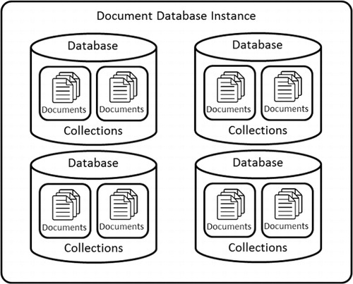
MongoDB is a document database modeled as a collection of objects which includes, from top to bottom, the database, collection, and document. Figure 3 depicts the objects included in MongoDB and their relationships. The documents in MongoDB are analogous to records in a traditional relational database and formated as key/value pairs in BSON format which is a binary format modeled after JSON. Collections are used to group similar documents in the database and are analogous to tables in a traditional database. The database is the highest level and is used to group sets of collections.

Figure 3. Overview of components in a document database.

Document databases are often referred to as schemaless databases, and when used to store hydrologic data they offer a great deal of flexibility. Since documents are typically modeled using the JSON format, it is possible to store a wide variety of data types. In the HydroCloud system, documents have been designed to store both vector and raster spatial datasets as well as time series data. Vector datasets are modeled as sets of vertices and raster datasets are modeled as JSON arrays. When storing time series data in the document database, care must be taken in the selection of the proper hierarchy. How the data is divided typically depends on the granularity of your data and how it will perform under various query scenarios. For example, consider a time series of stream gauge data where we need to store a site identifier, a time stamp, and two data values. One could design a collection for stream gauge data and have a single document to represent a time series for a particular site. When new values for the site come in, we could insert them to this document. An alternative method would be to have a collection for each individual site and store each new measurement as a separate document. The choice in this scenario depends on performance. In this example, if the primary method to query the data is based on a range query on the date, it would be more efficient to query relevant documents within a collection than to select within a document. Another aspect of document databases such as MongoDB that needs to be considered in the design phase is whether the database will be distributed or not. If the database is to be distributed across a number of nodes, it is not ideal to have very large and growing documents because individual documents must be confined to a single node.

The document schema for the HydroCloud data warehouse was divided into a number of separate databases to house each data-set. The databases were separated to allow the system to scale out in the future since the precipitation and stream flow databases will ultimately need to be extended to a system distributed across a number of nodes. Having each type of data in its own database offers the most flexibility when considering this type of scaling. The schema for the HydroCloud database is shown in Figure 4.

Figure 4. HydroCloud document database schema.

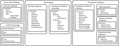
The HydroCloud data warehouse is divided into three primary document databases and a file system abstraction layer for very large documents. The three document databases include a stream flow database, precipitation database, and site information database. Within each database, data elements are stored as documents modeled using the JSON format. The document schema depicted in Figure 4 shows the layout of each document including the field names. Embedded fields are shown with their subfields indented. The symbol [] indicates that the data for a particular field is an array. For a detailed description of each document model, refer to the data dictionary shown in Table 1. The file system is implemented using GridFS which is a file system abstraction layer built on top of MongoDB that can be used for storing large documents that exceed the 16 MB size limit for BSON documents (MongoDB 2014a). In the HydroCloud database, the GridFS file system is used to store large image datasets including the NLCD. The flexibility in MongoDB allows documents to be modeled after JSON standards. For example, the following shows a GeoJSON document used to describe the catchment for site ID 01589000:

Table 1. Data dictionary for HydroCloud database.

Field Name	Data type	Description
Stream flow document
Site ID	String	USGS assigned site ID for stream flow gauges
Date/Time	ISO 8601 Timestamp (UTC)	Timestamp of stream flow measurement
Data	Embedded document	Embedded document to store stream flow measurement
Data.GaugeHeight	Double	Height of water surface measured in feet
Data.Discharge	Double	Stream flow measured in cubic feet per second
Precipitation grid document
Date/Time	ISO 8601 Timestamp (UTC)	Timestamp of precipitation grid
Precip grid	Array	4 km hourly NEXRAD precipitation accumulation grid for CONUS
Precipitation statistics document
Site ID	Text	USGS assigned site ID for stream flow gauge associated with document
Date/Time	ISO 8601 Timestamp (UTC)	Timestamp of precipitation grid
Basin average	Double	Hourly area averaged precipitation for catchment (mm/km^2)
Maximum	Double	Hourly maximum precipitation cell in basin (mm)
Minimum	Double	Hourly minimum precipitation cell in basin (mm)
Mean	Double	Hourly mean precipitation (mm)
Standard deviation	Double	Standard deviation of hourly precipitation in catchment (mm)
Percent coverage	Double	Percent of catchment covered by precipitation
Distance weighted	Double	Mean precipitation weighted by distance from stream gauge (mm)
Mask document
Site ID	String	USGS assigned site ID for stream flow gauge associated with document
Mask grid	Boolean array	Mask grid used to extract precipitation data for each catchment.
Spatial coordinate document
Latitude grid	Array	Array of latitude coordinates that correspond directly to precipitation grid
Longitude grid	Array	Array of longitude coordinates that correspond directly to precipitation grid
Site Info document
Site ID	String	USGS assigned site ID for stream flow gauges
Site name	String	Name of USGS stream flow gauge site
Site type	String	Type of site – in this application stream flow
Latitude	Double	Latitude coordinate of site
Longitude	Double	Longitude coordinate of site
State code	Double	State of site
Gage altitude	Double	Elevation of site
Drainage area	Double	Drainage area of site catchment
Contributing area	Double	Contributing drainage area to stream gauge
Catchment document
Type	Text	GeoJSON feature type
Geometry	Embedded document	Embedded document containing spatial feature
Geometry.Type	String	Spatial feature type
Geometry.Coordinates	List	Coordinates of the spatial feature
Properties	Embedded document	Embedded document containing attributes of spatial feature
Site ID	String	USGS assigned site ID for stream flow gauges
Area	Double	Area of polygon feature
Area units	String	Units of area field
Percent impervious	Double	Percent of catchment covered by impervious surface

{ “type”: “Feature”,

“geometry: {

“type”: “Polygon”,

“coordinates”: [[-74.239958305773570 43.981915607019829],

[-74.240323808107561 43.981976665508334],

[-74.240689311096773 43.982037722996381],

[-74.240774492143913 43.981775734641211],

...,

[-74.239958305773570 43.981915607019829]]

}

“properties”: {

“siteID”: “01589000”,

“area”: “41439.8”

“areaUnits”: “hectares”

“pctImpervious”:

}

Querying this document will result in a standard GIS format that can be used in most web-based mapping application programming interfaces.

The stream flow database contains a collection for each stream gauge site. Each individual measurement is then stored as a separate document. Storing each gauge’s measurements in a separate collection allows for more efficient range queries and updates. Also, this model gives us the ability to more easily distribute the data across multiple nodes so that we could ensure that documents belonging to the same collection are all on the same node. Each document contains the site ID, a time stamp, and a data key that contains a single gauge height and discharge measurement combined with a time stamp and site ID. It must be kept in mind that the database contains many similar documents for each NWIS gauge site. Each collection in the database is indexed based on the Date/Time field.

The site database consists of two document collections. The first contains metadata about the site including the site ID, the site name, site type, latitude, longitude, state code, gauge altitude, drainage area, and contributing area. The catchment collection contains the polygon features for each catchment associated with each NWIS stream gauge. Each catchment boundary is stored in its own document. The polygons are stored as a set of latitude and longitude pairs that begin and end on the same coordinate. Along with this information, the catchment document contains the area of the catchment and the area units. Finally, the percent impervious surface and percent forest cover values are calculated based on the NLCD contained in the GridFS File System. The site information collection and catchment collection are both indexed based on the Site ID field.

The precipitation database contains documents related to the collection and processing of the Stage IV precipitation data. This database contains four collections including the Stage IV precipitation grids, geographic coordinate grids, a set of mask arrays for each watershed which are used extract precipitation data for a given catchment, and a collection containing hourly precipitation statistics for each catchment. When the precipitation data is decoded from the grib file, latitude and longitude grids are also produced. The latitude and longitude grids assign each cell in the precipitation grid a set of geographic coordinates. The precipitation, mask precipitation, latitude, and longitude grids are stored as numerical arrays. The masks, latitude, and longitude grids are static and the hourly precipitation arrays are collected daily. The precipitation statistics collection contains documents for each site where each document contains the hourly precipitation statistics for a particular site and time stamp. The fact that the original precipitation arrays are stored in the database provides flexibility in that when new statistics and analysis methods are needed, the database can be extended to accommodate them. The precipitation grid collection is indexed on Date/Time and the mask collection and precipitation collection are both indexed on Site ID.

The GridFS file system is used to store geospatial images that are too large to be stored as BSON documents under normal MongoDB collections. Images can be easily read from the file system and used in ETL to characterize catchment areas. For example, in this version of HydroCloud, we are using the GridFS file system to store the United States NLCD (Homer, Fry, and Barnes 2012). These images are then used in the ETL process to calculate landscape characteristics for each catchment. This will be discussed in detail in the next section.

3.3. Extraction, transformation and loading

ETL is the process of extracting data from external sources, transforming the data based on system requirements, and loading the data into a data warehouse. The HydroCloud system runs ETL processes daily to update the NWIS stream flow data and the Stage IV precipitation grids and time series. The ETL workflows presented in this section are organized so that the source data are represented by the boxes on the left and processing steps and intermediate datasets are included in subsequent boxes. The ETL processing for the HydroCloud system was developed in the Python programming language. The ETL workflow for the NWIS stream flow data is presented in Figure 5. The NWIS stream flow data is available through a number of REST web service. The first web service that we call returns a list of site IDs that are used in subsequent web service requests. The first is the site information web service. This web service returns a comma separated value file that contains metadata about a particular stream gauge site. This web service is called only when a new site is added to the database. The ETL process first parses the csv file that is returned by the web service then encodes the information into a JSON document that is encoded to BSON and input into the site database.

Figure 5. ETL workflow for processing NWIS stream flow data.

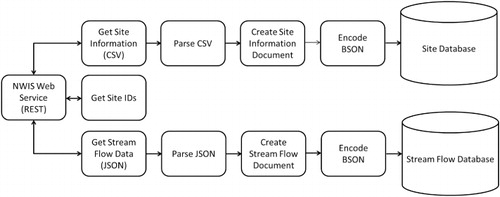
The NWIS system also includes a web service that returns flow data for a particular site. The flow data web service returns a JSON file that contains the values for a given time period. This web service is called daily where we include as a parameter the time period for the previous 24 hours. After calling the web service, the next step in the ETL process is to parse the JSON document and extract the data used to create the stream flow document. The stream flow document is then encoded into the BSON format and inserted into the stream flow database.

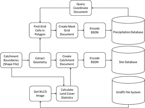
The USGS watershed boundary GIS files for NWIS sites are available in shape file format. The ETL workflow for loading the watershed boundaries into the HydroCloud data warehouse is presented in Figure 6. The watershed data consists of 18 shape files based on the USGS Water Resource Regions in the conterminous USA. The first step in this workflow is to extract the geometry for each watershed boundary in each shape file. After the geometry is extracted, the next step is to find the precipitation grid cells that fall within each polygon. To do this, a grid with cell values of all zero is created with the same dimensions as the precipitation grid. Then using the latitude and longitude values associated with the precipitation grid cells, the grid cells that fall within each watershed are given a value of 1 resulting in a mask grid of the watershed. For this, the coordinate arrays are reshaped to a 2 × n array consisting of a row for each latitude and longitude. Then ray casting is used to test whether each grid cell is within the watershed polygon. This results in a Boolean vector where 1 represents a set of coordinates that fall within the watershed and 0 outside the watershed. This vector is then reshaped into the original array format to create a mask of the watershed. The mask is applied in subsequent ETL processes to the precipitation grid to extract precipitation for each watershed. The catchment boundaries are also stored as documents in the database. These documents include the geometry of the catchment as well as the land cover statistics. The land cover statistics are generated by using the RasterStats package in Python. Using this package, the NLCD data is read from the GridFS file store and raster statistics are calculated based on each polygon in the shape file. These values are then added to the catchment document, encoded as BSON and inserted into the site database.

Figure 6. ETL workflow for processing watershed boundary GIS files.

The next step in the ETL workflow is to collect the Stage IV precipitation data and watershed boundaries and calculate the precipitation statistics time series. The ETL workflow for processing the precipitation data and creating the basin-averaged precipitation time series is shown in Figure 7. The Stage IV precipitation data is available over ftp in gridded binary (grib) format which is a data format commonly used by the meteorology community. The PyGrib Python API for grib data is used to decode the precipitation, latitude, and longitude grib files and convert them into arrays. These arrays are then used to create JSON documents for the precipitation grid, latitude grid, and longitude grid. These JSON documents are then encode to BSON and inserted into the precipitation database. The precipitation statistics are then extracted. To do this, the mask grid is queried for each NWIS site and the precipitation grid is masked. The resulting grid is then used to calculate the statistics for each stream gauge site.

Figure 7. ETL workflow for processing Stage IV precipitation data.

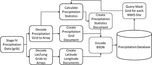
Included in the statistics are the NEXRAD cell with the maximum precipitation and minimum precipitation, the mean precipitation for the catchment, and the standard deviation for the catchment. The percent coverage statistic takes into consideration the percentage of the catchment that is receiving precipitation for a given time period and the distance weighted precipitation applies a distance weighted average to the precipitation where NEXRAD cells that are closer to the stream gauge location receive a higher weight and therefore contribute more to the average. The precipitation statistics document is then encoded to BSON format and inserted into the database.

3.4. Querying the HydroCloud database

Once the data is loaded into the HydroCloud database, there are a number of ways to query the data. The document database gives a tremendous amount of flexibility because the data can be queried from the system and integrated at the application layer. In particular, the MongoDB API has drivers available for a number of major programming languages including C, C++, Java, node.js, PHP, Perl, Python, and Ruby. In this implementation, the Python API is used to query the HydroCloud database and perform additional analysis on the data.

The queries that have been developed this far range from the very simple to the more complex. For example, one of the most useful queries that we have developed is a time series query that returns the precipitation statistics and flow data for a particular site so that they can be visualized. This query requires a date range and a site ID and returns a time series for flow and a time series for the precipitation statistics. An example time series query is shown using the Python API below. This query returns a precipitation time series with the average, minimum, and maximum precipitation for a site as well as a flow time series.

#import necessary python modules

import pymongo

import numpy

import pickle

def queryPrecipFlow(startDate, endDate, siteID):

#set up database connection

con = pymongo.Connection(<ip>,<port>)

precipCollection = con.precip.precipStats

flowCollection = con.flow.IDsiteID

#create precipitation time series

precipTS = []

#query precipitation time series collection

for precipDoc in precipCollection.find(recipCollectgt′: startDate,′ltʺtʺendDate}nsiteID’isiteID):

precipTS.append(precipDoc[recipDocprecipDoc[ravgPrecip’vgPrecip[[pend(precipDoc[[oc[iflowTS = []

#query stream flow time series

for flowDoc in flowCollection.find(lowCollectiogt′: startDate,′ltʺtʺendDate}nsiteID’isiteID):

flowTS.append([flowDoc[lowDoc[cflowDoc[ldata.discharge’a]])

As is evident from the above example, the document database exposes the data at the application level and gives a great deal of flexibility to the developer in terms of what can be done with the data once it is retrieved. For example, a developer could then easily use the Python matplotlib module to create a graph. An example graph created using this query combined with matplotlib is shown in Figure 8. Given a list of site IDs and a time range, a series of graphs can be automatically created for a large number of sites in a very short period of time.

Figure 8. Example precipitation and stream flow visualization created from sample database query.

More complex queries can obviously be envisioned with the HydroCloud database. Again, because the query is developed at the application level, query workflows can be created and then coded into custom applications. One example query workflow would be to select a set of stream gauges based on the percent impervious area of the catchment. Then take the resulting set of site IDs and use them as input to the time series query. This query could be even more elaborate where one could extract data for particular storms by querying the precipitation time series to return a set of time stamps where the precipitation reached a user-supplied threshold for each site. This merely illustrates the flexibility of the HydroCloud data structure and the ability to develop custom applications to perform data-driven hydrologic analysis.

3.5. Web services and user interface

We have included the time series query functionality in a web services interface that drives an exploratory user interface for the HydroCloud system. The HydroCloud system uses REST web services to provide access to the data stored in the data warehouse. The web services offer an extensible method to access the data warehouse and thus allow users to create their own programs for data analysis. An overview of the web services architecture for the HydroCloud system is depicted in Figure 9.

Figure 9. Overview of HydroCloud web service architecture.

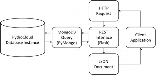
The web service architecture for the HydroCloud system was developed using the Python programming language where we use PyMongo as a query interface for the MongoDB data warehouse and Flask to provide a RESTful web service interface. Clients can access the NWIS stream flow and Stage IV precipitation web service interfaces using an http request where a query string is appended to the URL that identifies the site ID, start date, and end date of the time series. Figure 10 shows the JSON object returned from a web service request for the Stage IV precipitation data service for site 01585200 for the time period 1/01/2012 to 1/02/2012. In this example, we see the JSON object containing a precipitation value, a site ID, and a time stamp.

Figure 10. Example web service result showing Stage IV precipitation JSON return.

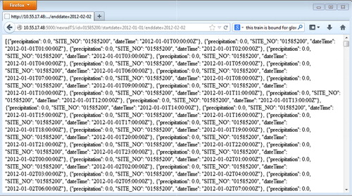
The NWIS stream flow web service URL is formated in the same way as the Stage IV precipitation web service and the JSON object. This offers modularity so that a single module can process data coming from both time series web services.

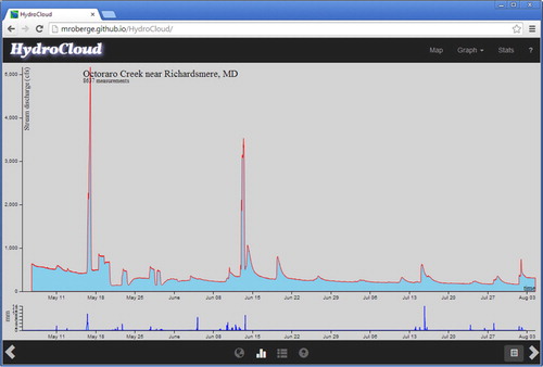
The HydroCloud client interface (http://hydrocloud.org) is implemented as a single-page web application written in JavaScript (code available from https://github.com/mroberge/HydroCloud) specifically for display in mobile phone web browsers. NEXRAD data were served from a HydroCloud instance in a private domain within the University, stream gauge data were requested directly from the USGS nwis.waterservices site, and the web client HTML was served from a Github pages site. The web interface consists of a mapping view (Figure 11), which allows users to find and request data, and a graphing view (Figure 12), which allows users to plot the requested data in several ways. The Knockout.js library (knockoutjs.com) is used to keep track of the view state and to update the UI; Google Maps JavaScript API v3 (https://developers.google.com/maps/web/) is used for the map interface; D3js (http://d3js.org/) is used for graphing, and Bootstrap (http://getbootstrap.com/) for HTML page styling.

Figure 11. HydroCloud web interface showing NWIS stream gauge locations and NEXRAD radar data.

Figure 12. HydroCloud web interface showing a plot of stream (top) and precipitation data (bottom).

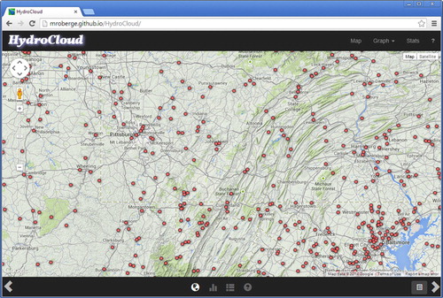
Users first interact with the HydroCloud client through the map view, which displays the location of USGS stream gauges as points over a background of the most recent NEXRAD image and a terrain basemap. When users click on a point, the client sends requests for both the stream gauge data and the basin-averaged NEXRAD precipitation time series data. The NEXRAD time series are requested from the HydroCloud data warehouse through the REST API, while the stream gauge data can request data from the HydroCloud data warehouse or optionally from the USGS service. The use of RESTful APIs makes it relatively simple to extend our current system to include other data services such as those provided by the NOAA National Climate Data Center’s Climate Data Online program.

Once the user has requested data through the map interface, the data are plotted immediately in the graph view as they arrive to the client. Users can choose different ways to graph the data, including a hydrograph, which displays stream gauge data from several sites on a common set of axes; a flow duration chart, which displays the data for a single stream gauge as a probability density function; a histogram, which displays the data for a single stream gauge in log-transformed bins; and a hyetograph, which allows the comparison of stream gauge data against the precipitation time series generated by the HydroCloud system from NEXRAD data.

3.6. HydroCloud web service performance

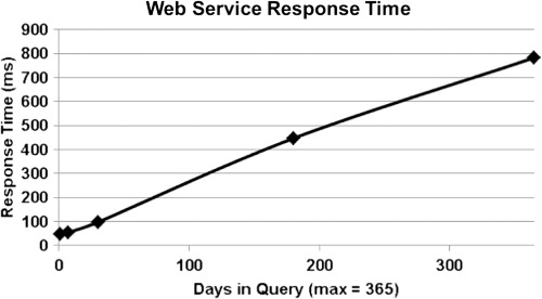
At its most basic level, the core of the HydroCloud system provides an integrated dataset consisting of time series of precipitation and stream flow aggregated at stream gauge locations. The web services that offer this data is the critical output of the system in that developers can incorporate these web services in mash-up applications. With this in mind, the performance of the web services were tested to determine the performance of the system when querying data with varying time ranges. The performance testing was performed using Google Chrome on a Dell Optiplex 990 desktop computer with 8GB of RAM and a 2.44 GhZ processor. To execute the performance test, the REST web service address was called using varying time ranges of 1, 7, 30, 180, and 365 days. The results of the performance test are shown in Figure 13. The web service response time generally scales linearly with the time range in the request with the response time for 1 day being almost instantaneous and 1 year of data taking 800 milliseconds, which equates to a response time that is still under 1 second.

Figure 13. Response time for HydroCloud web services.

4. Using the HydroCloud system for hydrologic analysis

The HydroCloud system can be used for both exploratory and statistical data analysis. This section will present an experiment where the HydroCloud system was used for a full scope of analysis from exploration to a statistical examination of the effect of urbanization on hydrology. For this demonstration, the web interface was used to select study sites and to identify storm events for the statistical analysis. The stream gauges were selected so that they would have a similar geologic setting (the central Maryland Piedmont) and would be close enough to each other to be subject to the same storm systems. The watersheds selected range in size from 36 to 739 km², and have 0.7% to 27% of the watershed area covered by pavement or other surfaces impervious to infiltration by rain. The list of selected sites is shown in Table 2.

Table 2. Sites selected for analysis of hydrologic response using the HydroCloud web interface.

Site ID	Site name	Area (km^2)	Percent impervious surface
01589000	Patapsco River at Hollofield, MD	739	3.1
01582500	Gunpowder Falls at Glencoe, MD	414	0.9
01594000	Little Patuxent River at Savage, MD	254	8.5
01580000	Deer Creek at Rocks, MD	244	1.4
01594526	Western Branch at Upper Marlboro, MD	234	16.0
01649500	Northeast Branch at Anacostia River at Riverdale, MD	188	20.0
01589352	Gwynns Falls at Washington Blvd. at Baltimore, MD	159	27.3
01583500	Western Run at Western Run, MD	156	0.7
01586000	North Branch Patapsco River at Cedarhurst, MD	145	4.2
01582000	Little Falls at Blue Mount, MD	139	0.9
01651000	Northwest Branch Anacostia River, Hyattsville, MD	128	19.2
01584500	Little Gunpowder Falls at Laurel Brook, MD	94	1.1
01581700	Winters Run near Benson, MD	90	2.7
01586610	Morgan Run near Louisville, MD	73	1.0
01589440	Jones Falls at Sorrento, MD	65	5.1
01583600	Beaverdam Run at Cockeysville, MD	54	13.2
01586210	Beaver Run near Finksburg, MD	37	3.4

Once the sites were selected, the next step was to use the graphing function of the HydroCloud interface to identify precipitation events for the analysis. Two storms were identified: A short but intense storm on 16 May 2014, and the much larger ‘Superstorm’ Hurricane Sandy, which peaked on 29 October 2012. The 16 May 2014 storm was a single, heavy downpour that flooded downtown Baltimore and nearby watersheds with single flood wave. This storm was selected because the timing of the rain and subsequent flood made it easy to identify what time the precipitation and flooding each reached their maximum for a modified ‘lag time’ analysis. Hurricane Sandy flooded the region mostly on 29 October 2012, and was selected for its massive size.

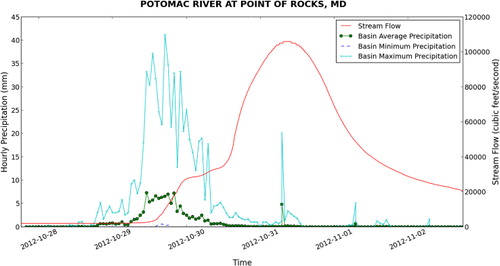
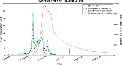
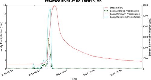
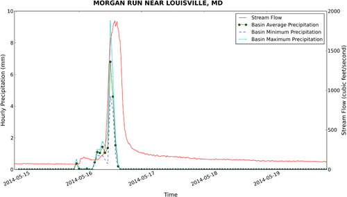
The web interface proved to be effective in the selection of sites and precipitation events for the analysis. However, a different approach was needed to develop custom visualizations of the precipitation and stream flow for a particular site and storm. For this, we used the hydrologic analysis and visualization tools developed in Python to query the database for a given time range and site and to automatically generate plots for each site similar to that shown in Figure 8. This visualization exercise will guide the analysis in that it will show the relationship between the precipitation statistics and stream flow for a given watershed. For example, Figures 14 and 15 show the visualization for the Patapsco River at Hollofield, MD which is the largest watershed in the analysis. Here, we can see that the watershed responds differently to each event, where Hurricane Sandy produced a more sustained hydrograph with two peaks between 8000 and 10,000 cfs, while the 16 May 2014 storm produced a fast pulse in stream flow of approximately 6000 cfs.

Figure 14. Hydrograph and precipitation statistics for the Patapsco River at Hollofield, MD for Hurricane Sandy (29 October 2012).

Figure 15. Hydrograph and precipitation statistics for the Patapsco River at Holofield, MD for May 2014.

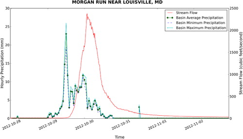
If we look at a smaller watershed such as Morgan Run near Louisville, MD shown in Figures 16 and 17, we see a similar pattern except with lower flows. This suggests a correlation between watershed area and stream discharge. Also, if we look at the figures, there appears to be a correlation between the size of the watershed and the length of the lag time between the peak of the precipitation time series and the peak of the stream flow time series. Based on this, we would like to take the analysis further to test for statistical relationships between each time series.

Figure 16. Hydrograph and precipitation statistics for Morgan Run near Louisville, MD Hurricane Sandy (29 October 2012).

Figure 17. Hydrograph and precipitation statistics for Morgan Run near Louisville, MD for 16 May 2014.

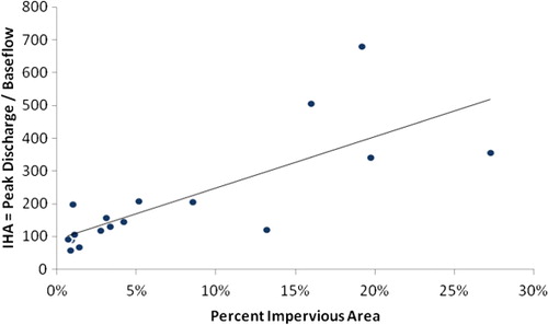
For the statistical analysis, we developed analysis tools in Python to calculate the stream discharge before the flood (also known as the baseflow), the peak discharge at the height of the flood, the total amount of precipitation that fell in the watershed, and the total amount of water discharged from the watershed. For the May 2014 storm, we also measured the lag time, which for this study we defined as the length of time between when the rain reached its peak intensity, and when the flood reached its peak discharge. From these measured variables, we calculated several derived statistics, including the percent runoff (volume of stream flow/volume of rainfall) and the Index of Hydrologic Alteration (IHA; the peak discharge/the base flow before the storm). Once the program was created to perform these analyses, we submitted the list of site IDs and the time range for each storm as input to the program. Then, using the output, linear regression was used to analyze the statistical relationships between the variables.

The regression analysis revealed several statistically significant relationships among the two independent variables (watershed area and percent impervious area) and the 13 dependent variables (two storm events times six measurements: total precipitation volume, total stream discharge volume, base discharge, peak discharge, IHA, percent runoff; plus lag time for the May storm) as shown in Table 3. As expected, watershed area was an important explanatory variable during both storms so that larger watersheds collected significantly more precipitation, leading to greater volumes of stream water, higher flood peaks, and higher base flow discharges. The percent impervious area did little to improve these results, and had no significant impact on these variables on its own.

Table 3. Statistical significance of relationships.

		p value		adj. R ^2
Independent	Dependent variable	May value	Sandy value	May value	Sandy value
Watershed area	Total stream discharge	<0.001	<0.001	0.95	0.74
	Total precipitation	<0.001	<0.001	0.96	0.92
	Base discharge	<0.001	<0.003	0.80	0.42
	Peak discharge	0.018	0.006	0.27	0.37
	(Index of Hydrologic Alteration)	0.336	0.778	−0.00	−0.06
	% Runoff	0.043	0.008	0.19	0.34
	(May lag time)	0.09		0.13
% Impervious	Index of Hydrologic Alteration	0.002	<0.001	0.46	0.56

Note: Insignificant relationships are in parentheses.

The amount of impervious surfaces in a watershed did have a significant impact on the IHA (Figure 18). The IHA partially removes the effect of watershed area by dividing peak discharges by base discharges; both of these variables correlate with watershed area. The IHA also exacerbates the effect of urbanization; urban, highly impervious watersheds are expected to have a lower base flow and a higher peak flow than rural watersheds. Dividing one by the other increases the sensitivity of this measure to the effects of urbanization.

Figure 18. The effect of percent impervious area on the index of hydrologic alteration. Based on data for 29 October 2012 (Hurricane Sandy) and 17 watersheds in central Maryland Piedmont.

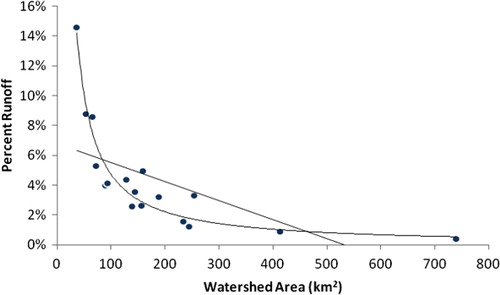
Watershed area also had a statistically significant effect on the percent runoff (Figure 19). Smaller watersheds had as much as 14% of their precipitation generate stream flow, while larger watersheds could produce less than 1%. This relationship was non-linear; when the watershed area was transformed using an inverse formula (predicted % runoff = 4.9/area), it produced a significant (p < 0.001) relationship where variations in the transformed watershed area explained 91% of the variation in % runoff.

Figure 19. The effect of watershed area on percent runoff. Percent runoff is calculated as the ratio of total stream discharge to the total volume of precipitation during Hurricane Sandy.

5. Discussion

The work presented in this paper uses MongoDB, a document-oriented NoSQL database, as a back end platform for the integration of hydrologic data. The use of NoSQL databases in digital earth research shows promise because of their ability to flexibly model heterogeneous datasets. Because of this, research in NoSQL databases shows tremendous potential. However, as with any new technology, there are advantages and disadvantages of using NoSQL databases instead of traditional relational database management systems. In this section, we discuss a number of advantages and drawbacks of using MondoDB for this application. We also discuss a number of potential application extensions where this technology can potentially support other types of digital earth research.

5.1. Advantages, drawbacks, and limitations

One advantage of using MongoDB for the HydroCloud application is the flexibility that it offers in integrating additional data types without having to completely redesign the schema. Also, because the nature of a document database allows documents to be distributed across a number of nodes, the database therefore can easily be scaled out to a distributed model. Also, from the standpoint of a developer, MongoDB offers a rich query language that lends itself well to dynamic programming languages such as JavaScript and Python. This could potentially be seen as a drawback in that it does not support SQL, but the fact that queries can be executed using an API replaces the need to create complex query strings to go between the application and the database. This allows for more convenient access to the data. Another criticism of the MongoDB query language is that join operations are not supported. However, in our experience, joins can be done by reference at the application layer with multiple queries. MongoDB also supports a number of index types including spatial indexes. Finally, because of the extreme write load required for writing the NEXRAD arrays, MongoDB supports very fast write performance.

There are also a number of disadvantages to using MongoDB as a backend database that must be mentioned. While the flexibility of a schemaless database was generally viewed to be positive in the case of this application, it could be a big drawback considering that it lacks support for the reliable processing of transactions. In essence, if a transaction is aborted before it is completed, that data is lost. This can be accounted for by using replication. However, this also requires additional computational resources. In the case of the HydroCloud system, durability is not a concern since the system is being used for integration, warehousing, and offline analysis of hydrologic data. Another issue that became apparent when implementing the HydroCloud system is that in MongoDB, indexes take up a large amount of space. To account for this unforeseen requirement, more space had to be added to the server. Also, MongoDB does not support transactions and therefore is not as durable as a traditional RDBMS. Another disadvantage could be the lack of a high level query language such as SQL. However, we must note that we found that pyMongo, MongoDB’s query API for Python, supported all of the query functionality that was required for the HydroCloud application.

The prototype that was developed as a part of the HydroCloud system also has a number of limitations associated with processing the NEXRAD precipitation data. For example, the initial design included the ability for researchers to integrate precipitation based on any user-supplied catchment and it is still desirable to extend the system to include this functionality. However, while this is possible at the application layer, the performance of the algorithm used to find all grid cells that fell within a polygon boundary had dismal performance when processing large watersheds. Because of this, we adopted the masking technique where the watershed is masked and precipitation cells are selected using this mask in the ETL process. This is also the reason why the precipitation time series document collection was created. Another challenge that was experienced in the development of the HydroCloud system was the combination of many open source technologies for the end-to-end system. On the backend of the system, this included Python modules for decoding GRIB files, extraction translation and loading data into MongoDB, and implementing the necessary queries as web services. On the web client side, this included a number of JavaScript libraries for data visualization, web mapping, and navigation.

5.2. Potential application extensions

The technology used in the HydroCloud system can be applied to any analysis that requires the integration of spatial and temporal data from multiple sources. For example, dissolved oxygen readings taken over time at moored buoys might be combined with satellite imagery of chlorophyll concentrations to support real-time investigations of algae blooms in large water bodies such as the Chesapeake Bay.

Alternatively, our system could be modified to allow the exploratory analysis of agricultural crop production data. Each month the USDA National Agricultural Statistics Service produces reports on crop production based on the number of acres planted or harvested and the yield per acre. This information is of great importance to the agricultural futures market and to farmers in other regions, who decide what to plant based on these estimates of how much will be produced elsewhere. Our system could combine raster-based Normalized Vegetation Difference Index measurements taken from satellites with vector-based field outlines and temporal data from weather stations. By simply modifying the ETL process and the front end to collect data from different sources, analysts could use our system to browse through weather data and satellite imagery to estimate the impact of drought or heavy storms on crop yields.

6. Conclusion

This paper presents a system for the integration of hydrologic data for the analysis of watershed response to storm events. The HydroCloud system is based on a flexible document database design implemented in MongoDB. Furthermore, the system is novel in that it is the first to spatially integrate Stage IV NEXRAD precipitation data with NWIS stream flow data in a single system. A set of ETL workflows were presented to show the steps taken to integrate the data in the document database. The resulting database offers an extreme amount of flexibility and allows programmers to easily create custom hydrologic analysis functions. A set of RESTful web services provide access to the HydroCloud integrated data-set, and exploratory analysis can be performed on desktop computers and mobile devices using a light-weight web interface. The utility of the HydroCloud system was demonstrated in an exploratory analysis of watershed response that produced interesting results related to the impact of catchment size and imperviousness. With this in mind, there are a number of future enhancements that we would like to apply to the HydroCloud system. First, the database and web services are currently implemented in a testing environment on an internal network. We would like to port the database to a more robust environment to increase its availability. We would also like to develop additional query tools to facilitate analysis such as the identification and analysis of storm events, time series analysis of rainfall and runoff signals, and spatial statistical analysis of precipitation grids. Finally, we would like to extend the web services to include more complex queries on the precipitation and stream flow datasets and incorporate a more elaborate query interface into the web front end.

Disclosure statement

No potential conflict of interest was reported by the authors.

Additional information

Funding

This work was supported by the Towson University School of Emerging Technologies.

References

- Aji, A., and F. Wang. 2012. “High Performance Spatial Query Processing for Large Scale Scientific Data.” In Proceedings of the on SIGMOD/PODS 2012 PhD Symposium - PhD ’12, 9. New York: ACM Press. http://dl.acm.org/citation.cfm?id=2213598.2213603.
- Aji, A., F. Wang, and J. Saltz. 2012. “Towards Building a High Performance Spatial Query System for Large Scale Medical Imaging.” In Proceedings of the 20th ACM SIGSPATIAL International Conference on Advances in Geographic Information Systems, Redondo Beach, California, USA.
- Akdogan, A., U. Demiryurek, F. Banaei-Kashani, and C. Shahabi. 2010. “Voronoi-based Geospatial Query Processing with MapReduce.” In 2010 IEEE Second International Conference on Cloud Computing Technology and Science, IEEE, ISBN 978-1-4244-9405-7, 9–16. http://ieeexplore.ieee.org/xpl/freeabs\_all.jsp?arnumber=5708428.
- Ator, S., J. Brakebill, and J. Blomquist. 2011. Sources, Fate, and Transport of Nitrogen and Phosphorus in the Chesapeake bay Watershedan Empirical Model: U.S. Geological Survey Scientific Investigations Report 20115167, Technical report. http://pubs.usgs.gov/sir/2011/5167/.
- Brezany, P., Y. Zhang, I. Janciak, P. Chen, and S. Ye. 2011. “An Elastic Olap Cloud Platform.” In 2011 IEEE Ninth International Conference on Dependable, Autonomic and Secure Computing, IEEE, ISBN 978-1-4673-0006-3, 356–363. http://ieeexplore.ieee.org/xpl/freeabs\_all.jsp?arnumber=6118761.
- Cao, Y., C. Chen, F. Guo, D. Jiang, Y. Lin, B. C. Ooi, H. T. Vo, S. Wu, and Q. Xu. 2011. “Es2: A Cloud Data Storage System for Supporting Both oltp and olap.” In Data Engineering (ICDE), 2011 IEEE 27th International Conference on IEEE, 291EE.
- Chiang, G., M. T. Dove, C. I. Bovolo, J. Ewen, X. Yang, L. Wang, and W. Jie. 2011. “Implementing a Grid/Cloud escience Infrastructure for Hydrological Sciences.” In Guide to e-Science, edited by Yang, X., L. Wang, and W. Jie, 3–28. London: Springer, Computer Communications and Networks, ISBN 978-0-85729-438-8. http://www.springerlink.com/content/j2mrp613v3802527/.
- Goodall, J., J. Horsburgh, T. Whiteaker, D. Maidment, and I. Zaslavsky. 2008. “A First Approach to Web Services for the National Water Information System.” Environmental Modelling & Software 23: 404. doi:10.1016/j.envsoft.2007.01.005.
- Han, Y.-H., D.-S. Park, W. Jia, and S.-S. Yeo, eds. 2013. Ubiquitous Information Technologies and Applications, Lecture Notes in Electrical Engineering, volume 214. Dordrecht: Springer. http://www.springerlink.com/index/10.1007/978-94-007-5857-5.
- Heard, J. R. 2011. Geoanalytics, Technical report, Renaissance Computing Institute. http://www.renci.org/wp-content/uploads/2011/03/TR-11-03.pdf.
- Homer, C. H., J. A. Fry, and C. A. Barnes. 2012. The National Land Cover Database. US Geological Survey Fact Sheet 3020, 1–4.
- Horsburgh, J. S., D. G. Tarboton, M. Piasecki, D. R. Maidment, I. Zaslavsky, D. Valentine, and T. Whitenack. 2009. “An Integrated System for Publishing Environmental Observations Data.” Environmental Modelling & Software 24: 879. doi:10.1016/j.envsoft.2009.01.002.
- Krajewski, W. F., A. Kruger, J. A. Smith, R. Lawrence, C. Gunyon, R. Goska, B. C. Seo, P., et al. 2011. “Towards Better Utilization of NEXRAD Data in Hydrology: An Overview of Hydro-NEXRAD.” Journal of Hydroinformatics 13: 255–255. doi:10.2166/hydro.2010.056.
- Lin, Y., and K. E. Mitchell. 2005. “The NCEP Stage ii/iv Hourly Precipitation Analyses: Development and Applications.” 19th Conference on Hydrology, American Meteorological Society, San Diego, CA, 9–13, January 2005.
- Lu, S., R. M. Li, W. C. Tjhi, K. K. Lee, L. Wang, X. Li, and D. Ma. 2011. “A Framework for Cloud-based Large-scale Data Analytics and Visualization: Case Study on Multiscale Climate Data.” In 2011 IEEE Third International Conference on Cloud Computing Technology and Science, IEEE, 618–622. http://ieeexplore.ieee.org/articleDetails.jsp?arnumber=6133204\&contentType=Conference+Publications.
- Maidment, D. 2006. “Hydrologic Information Systems.” AGU Fall Meeting Abstracts, -1, 1209. http://adsabs.harvard.edu/abs/2006AGUFMIN21A1209M.
- Maidment, D. R. 2002. ArcHydro: GIS for Water Resources. ESRI Press.
- McGuire, M. P., M. C. Roberge, and J. Lian. 2014. “Hydrocloud: A Cloud-based System for Hydrologic Data Integration and Analysis.” In Computing for Geospatial Research and Application (COM. Geo), 2014 Fifth International Conference on, 9–16, IEEE.
- McGuire, M. P., and R. Sanderson. 2010. HydroNEXRAD Data for Gwynns Falls and Baisman Run Watersheds. http://oshydro.umbc.edu/GFhydroNEXRAD/.
- MongoDB. 2014a. GridFS, online. http://docs.mongodb.org/manual/core/gridfs/.
- MongoDB. 2014b. MongoDB. https://www.mongodb.org/, URL https://www.mongodb.org/.
- Svoma, B. M., and R. C. Balling. 2010. “United States Interannual Precipitation Variability over the Past Century: Is Variability Increasing as Predicted by Models?” Physical Geography 31: 307. doi:10.2747/0272-3646.31.4.307.
- Thusoo, A., J. S. Sarma, N. Jain, Z. Shao, P. Chakka, N. Zhang, S. Antony, H. Liu, and R. Murthy. 2010. “Hive - A Petabyte Scale Data Warehouse Using Hadoop.” In 2010 IEEE 26th International Conference on Data Engineering (ICDE 2010), IEEE, ISBN 978-1-4244-5445-7, 996–1005. http://ieeexplore.ieee.org/xpl/freeabs\_all.jsp?arnumber=5447738.
- United States Geological Survey. 2011. USGS Streamgage NHDPlus Version 1 Basins 2011. http://water.usgs.gov/GIS/metadata/usgswrd/XML/streamgagebasins.xml.
- United States Geological Survey. 2014. USGS Water Data for the Nation. http://waterdata.usgs.gov/nwis.
- Yang, C., M. Goodchild, Q. Huang, D. Nebert, R. Raskin, Y. Xu, M. Bambacus, and D. Fay. 2011. “Spatial Cloud Computing: How can the Geospatial Sciences Use and Help Shape Cloud Computing?” International Journal of Digital Earth 4: 305–329, ISSN 1753-8947. doi:10.1080/17538947.2011.587547.