Horizontal accuracy assessment of very high resolution Google Earth images in the city of Rome, Italy

Abstract

Google Earth (GE) has recently become the focus of increasing interest and popularity among available online virtual globes used in scientific research projects, due to the free and easily accessed satellite imagery provided with global coverage. Nevertheless, the uses of this service raises several research questions on the quality and uncertainty of spatial data (e.g. positional accuracy, precision, consistency), with implications for potential uses like data collection and validation. This paper aims to analyze the horizontal accuracy of very high resolution (VHR) GE images in the city of Rome (Italy) for the years 2007, 2011, and 2013. The evaluation was conducted by using both Global Positioning System ground truth data and cadastral photogrammetric vertex as independent check points. The validation process includes the comparison of histograms, graph plots, tests of normality, azimuthal direction errors, and the calculation of standard statistical parameters. The results show that GE VHR imageries of Rome have an overall positional accuracy close to 1 m, sufficient for deriving ground truth samples, measurements, and large-scale planimetric maps.

Keywords:

• Google Earth
• VHR images
• GPS
• accuracy assessment
• Rome

1. Introduction

In recent years, the advent of freely available virtual globes, such as Google Earth (GE), NASA World Wind, Microsoft Bing Maps, and others, has opened a new era of Digital Earth (DE) (Goodchild et al. 2012), enabling users exploring satellite and aerial images and to address geographical issues (Lin, Huang, and Lu 2009). In particular GE (http://www.google.com/earth/index.html), shortly after its release in 2005, has evolved along with its increasing interest and popularity due to the free access, user-friendly interface, and richness of content at global coverage, showing a realistic and engaging view of the surface of the planet. As a result of its popularity, also an increasing number of researchers have recently begun using GE images for several applications in technical and scientific projects. A brief search on peer-reviewed journal papers, by using the Institute of Scientific Information databases and Google Scholar, reveals over 100 relevant articles with the term ‘Google Earth’ on titles, abstracts or keywords, while many others mentioned it on full-length text. The use of GE by the scientific community pertains to studies on Land use/Land cover (LULC), agriculture, Earth surface processes, biology, landscape, habitat availability, health and surveillance systems, etc. Research applications harnessing GE features were summarized by Yu and Gong (2012) into eight categories: data collection, validation, visualization, data integration, modeling, communication, dissemination, and decision support. Uses of GE for data collection and validation are particularly interesting in remote sensing applications and increasingly being used in conjunction with image processing methods for LULC mapping and forest inventories. For instance, the potential of GE images have been demonstrated by Taylor and Lovell (2012) to detect urban agriculture areas in the city of Chicago with a relatively high accuracy. GE was used by Dorais and Cardille (2011) and Dong et al. (2012) to extract ground truth data and used as a training and test sample to aid and evaluate classification datasets derived from MODIS and PALSAR images. Similarly, GE images were used by Cracknell et al. (2013) to classify land cover classes within 1-km spatial resolution MODIS pixel, while accuracy assessment of global urban map was carried out by Potere et al. (2009). Ploton et al. (2012) successfully modeled and assessed aboveground biomass of tropical forest using GE canopy images, highlighting the great potential of the method for biomass retrieval. They also propose the first reliable map of tropical forest aboveground biomass in the Western Ghats of India by using GE images. Sato and Harp (2009), Fisher et al. (2012) and Frankl et al. (2013) all demonstrated the usefulness of high spatial resolution GE images in the study of Earth surface to yield quantitative insights about geomorphological processes like landslides, channel-width variability, and gully erosion. Wang, Huynh, and Williamson (2013) integrated GE data with a microscale meteorological model to improve its functionality and ease of use. They also developed modular software to convert model results and intermediate data for visualizations and animations with GE. Similarly, GE has been used to visualize seismic tomographic data (Yamagishi et al. 2010) and meteorological satellite data (Chen et al. 2009). In addition, uses are reported in multidisciplinary research on habitat for endangered bird species (Benham et al. 2011), changes in snow and glacier cover (She et al. 2014), dengue surveillance system (Chang et al. 2009), estimates of fish catches (Al-Abdulrazzak and Pauly 2013), and archeological studies (Contreras and Brodie 2010) to name just a few recent studies. Despite this large penetration of GE use for scientific projects, many open research questions can be raised concerning the reliability of the imagery, since very few information are released by Google Inc. on metadata about sensors, image processing and resolutions, overlay techniques, etc. In particular, one of the major drawbacks is related to uncertainty on horizontal accuracy that might limit the scientific use of these data and lead to misinterpretations of the results and incorrect inferences, especially on area estimates and data retrieval applications (McRoberts 2010). However, to date, despite the potential of these images, very few studies were aimed at assessing the horizontal accuracy and their geo-positioning capability for maps creation in the field of DE. The first systematic study on positional accuracy was reported by Potere (2008), who determined the absolute accuracy of GE images at a global scale for several worldwide places. In another study, Paredes-Hernandez et al. (2013) undertook the accuracy assessment at a regional scale over rural areas in Mexico. Similarly, in a study about direct orthorectification of raw satellite images, Yousefzadeh and Mojaradi (2012) validated the accuracy of GE images in two test sites before using them to extract planimetric ground control and check points (CPs). To the best of our knowledge, there is a lack of investigations and analysis on positional accuracy of very high resolution (VHR) GE images, especially in metropolitan areas, where greater are the updates and resolutions of the images provided by Google Inc. The overarching goal of this paper is to investigate the horizontal accuracy of VHR GE images in the city of Rome, using both cadastral photogrammetric measurements and GPS (Global Positioning System) ground truth data as CPs. The findings should make an important contribution to expand the use and sharing of geo-referenced web data in the growing area of DE. Robust statistical inference procedure follows a comparison of East and North coordinates between the candidate CPs and their equivalent corresponding points displayed by GE. Hence, a set of statistical parameters and confidence intervals were calculated to summarize positional error starting from selected CPs. The following sections describe the datasets and the workflow of the assessment procedure, then a discussion explaining the results in relation to a potential uses of the images is provided.

2. Materials and methods

2.1. Study area and data description

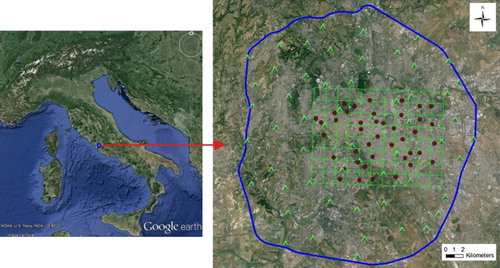
The study area is the city of Rome, which is the most populous of Italy, covering more than 1280 km² with a population of about 2,65 million inhabitants. Specifically, it was decided to assess the horizontal accuracy of the area that totally falls within the Grande Raccordo Anulare (GRA), centered on the geographic coordinates 41° 54′ 00″ North latitude and 12° 30′ 00′ West longitude. GRA is a ring-shaped orbital highway that encircles Rome urban area, covering an area of about 344 km² and 63 km in circumference (Figure 1). The study area has a flat or slightly wavy relief, and the elevation ranges from 3 m up to 140 m above sea level with mean value close to 46 m.

Figure 1. Study area in GE. The blue line represents the GRA, the green grid represents the GPS survey area. Green points and red points represent the cadastral and GPSs CPs, respectively.

2.1.1. GE imagery

GE is the most popular virtual globe software that visualizes images as a global mosaic of the Earth of mid and high-resolution satellite and aerial imagery from multiple providers, including ancillary data-like pictures, address, etc. Moreover, it enables users to create geometric primitives such as points, lines, polygons, and attributes such as vector format Keyhole Markup Language (KML). The type of images displayed depend on the zoom level for a specific area, ranging from SPOT5 and Landsat images for continental-scale view or deserts, rainforests, and poles, up to aerial orthophotos, IKONOS, QuickBird, GeoEye-1, Worldview-1, and Worldview-2 images for urbanized areas to the maximum zoom level. The only metadata available are reported when a user zooms on a specific zone by displaying in the bottom part of the window the name of data provider and the acquisition date. Starting from the GE version 5, there is also the possibility to browse archival images, which allows to assess temporal changes. The Ground Sample Distance (GSD) and images resolution can be estimated only considering the dimension of features observed. In this paper, we evaluate the images dated 17 June 2013, 10 November 2011, and 29 July 2007, due to the comparable GSD and pixel dimension, about 30 cm, that seem to be aerial images. The spatially extension of these images totally falls within the GRA without mismatched or seam with other images.

2.1.2. Cadastral points

The data-set is composed of points of certified coordinates selected from the Italian Cadastre and known as ‘Punti Fiduciali’ (PF). These points are part of the Italian cadastral mapping system and constitute the positional reference for updating the cadastral maps. They are continuously updated according to a common technical procedure with the participation of professional engineers and land surveyors from National Boards of Professional Associations. The measurements, after bundle adjustments, are sent to the cadastral authorities in order to build up a collection of certified data (Barbarella 2014). Each point has an associated code and metadata that describes the process of coordinates generation, depending on the precision, survey methodologies and equipment used. In order to provide the benchmark to infer horizontal accuracy, 57 PF points have been selected from the web-mapping system repository (Globogis – http://ags.globogis.it/fiduciali_gfmaplet/?map=ortofoto). The coordinates of these points are generally acquired with total stations by reference to existing points from trigonometric vertices established by the Italian Military Geographic Institute. No information is available regarding the accuracy of the individual PF, but only a generic quality information that refers to minimum standards of accuracy established by the Italian Cadastre.

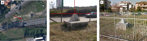
The coordinate reference system is WGS-84 UTM zone 33N, but originally they were represented in the local Cassini-Soldner projection, used for mapping areas with limited longitudinal extent. The points selected, homogeneously distributed in the GRA area, are located on isolated small objects, curbsides or corners of small artifacts which are presumed to be stable over the time, in order to ensure a fast and reliable identification of locations (Figure 2).

Figure 2. The location of the PF vertex: (a) GE image, (b) cadastral monograph, (c) Google Street view image. The CP is a manhole cover of an aqueduct.

2.1.3. GPS points sampling

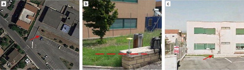
The GPS data-set consists of 41 CPs that were collected during several measuring campaigns, also suitable as ground control data to orthorectify satellite imagery and aerial photographs. Due to the difficulty and costs to execute a survey extended all over the GRA area, the collection of data was concentrated in the city center, covering about 88 km² (see Figure 1). The search for accessible and easily recoverable points was carried out carefully, in order to guarantee a homogeneous and randomly spatial distribution over the study area and best coverage of the GPS signal (Figure 3). In fact, when using GPS receivers on urban environment must be avoided the urban canyon effect, resulting in poor GPS signal reception (Marais and Godefroy 2006). The network of points was surveyed in rapid-static mode with baseline length limited to 10 km, to prevent degradation in the accuracy of observations. The Position Dilution of Precision was always ≤4. A Topcon Legacy-E double-difference GPS/Global Navigation Satellite System (GNSS) receiver was used as rover to log all GPS point, while the permanent stations of GNSS Lazio Region and of National Institute of Geophysics and Volcanology were used as reference. The GPS data were taken from previous points and new points logged between March and July of 2013. A logging rate of 15 minutes was adopted throughout data acquisition at each point, during which the weather condition was favorable without cloud cover. The coordinate reference system is WGS-84 UTM zone 33N, the planimetric accuracy at each point is less than 2.5 cm while the orthometric heights (not used in this experiment) were estimated using ITALGEO05 Geoid model.

Figure 3. The location of the GPS vertex: (a) GE image, (b) GPS survey, (c) Google Street view image. The red arrows show the ground control target where the GPS receiver was positioned to obtain the horizontal coordinates. The CP is a curb ramp of parking.

2.2. Accuracy assessment

The positional accuracy of spatial data can be defined through measures of the difference between the location of the recorded feature and the true location (Goodchild and Hunter 1997). The National Standard for Spatial Data Accuracy (NSSDA) from the US Federal Geographic Data Committee (FGDC 1998) established the most widely used guidelines for positional accuracy inferences of spatial datasets like orthoimages and maps. It states that an independent source should be used for testing and reporting positional accuracy, defining accuracy as a measure of the maximum error expected at a probability level of 95% (Congalton and Green 2009). We calculated the magnitude of absolute and relative errors of GE images using standard statistical parameters provided by NSSDA. Absolute accuracy is measured as the error between the coordinates of CPs on the image and the coordinates of the points collected by GPS and PF. Absolute accuracy is expressed as the horizontal root mean-square error (RMSE), which is an overall indicator of the cumulative result of all errors. This includes both random and systematic errors introduced during the data generation process (ASPRS 1990). The relative horizontal accuracy is especially important for derivative products that make use of the local differences among adjacent horizontal values, such as area calculation. An image with good relative accuracy is one that accurately represents the shape of the terrain or distance and direction between two well-defined points, but may not necessarily be accurately registered to real geographic coordinates. The relative accuracy can be expressed as the confidence level that fulfills the RMSE requirement suitable for the production of planimetric maps. For accuracy testing, CPs selected must satisfy the following conditions (FGDC 1998):

• The points must be collected by an independent data source and with high accuracy;

• The points must be evenly distributed over the geographic extent of the image;

• The points must be well defined, easily identifiable and recoverable.

The number of CPs identified and collected within the study area (57 PF and 41 GPS points) is sufficiently large to guarantee error control reliability. In fact, the guidelines of FGDC states that to evaluate the accuracy of spatial data, at least a minimum of 20 independent CPs shall be tested. Similarly, the American Society for Photogrammetry and Remote Sensing (ASPRS 2013) recently developed new geo-location accuracy standards for digital geospatial data and recommend 20 clearly defined CPs for a project area ≤500 km². Nevertheless, Aguilar, Aguilar, and Agüera (2007) stated that 16–32 CPs are needed for constructing an RMSE with an accurate 95% confidence interval, while in the worst-case scenario (nonnormally distributed errors, areas of complex topography) 64–128 CPs are needed. It is clear that a greater number of CPs ensures a more complete and reliable statistical analysis (Cuartero et al. 2010), in accordance with some authors who suggest larger samples (Ariza and Atkinson 2005; Aguilar et al. 2012). To accomplish these goals and minimize spatial autocorrelation, CPs have been well distributed throughout the project area, spaced at intervals of at least 1/10^th the diagonal distance across the data-set. This ensures that at least 20% of the points are located to each quadrant (ASPRS 1990) (Figure 1). A square matrix of 1 × 1 km (Figure 1) was superimposed in GE to guarantee the minimum distance condition among selected points. Hence, in order to extract the coordinates of PFs, we firstly selected the candidate point from Globogis web-map and the corresponding position on GE. By clicking on the point, it displays a window with metadata, including the coordinates in WGS-84 that were copied and pasted in a spreadsheet. Another link allows to view the descriptive monograph, which shows the perspective pictures of the exact location of the points. In addition, the geo-referenced images of Google Street View, thanks to panoramic views along the streets (Figure 2), were used to correctly identify and position the PFs. Secondly, in GE was added a placeholder that represents the same candidate point from Globogis, and by using the zoom slider increased the view to the highest level at the represents PF point (Figure 4). Lastly, Easting and Northing coordinates were copied and pasted in a spreadsheet.

Figure 4. The zoomed image shows the location of the PF vertex represented in Figure 2 in the image 2007. Notice the pixel displacement between the positions of the data image coordinates and their corresponding position of the CP.

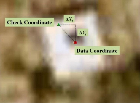
In fact, the placeholder on GE once saved as KML file do not remain in the position shown, but is placed as an object at the vertices of a square of side 1 × 1 m. A similar procedure was followed for the GPS points, firstly copying and pasting in a spreadsheet the coordinates collected from the survey, then adding a placeholder in GE to retrieve Easting and Northing coordinates that were copied and pasted in a spreadsheet. The positional accuracy was calculated for the three images (2007, 2011, and 2013) using either PF or GPS points. The accuracy of the image 2007 is determined as the difference between the PFs and image coordinates (pixel) and is denoted as GE07 – PF, while the accuracies for the images 2011 and 2013 are denoted as GE11 – PF and GE13 – PF, respectively. Similarly, the same procedure was followed using GPS points and the differences are denoted as GE07 – GPS, GE11 – GPS, and GE13 – GPS. Graphical data exploration and descriptive statistics of all datasets have been analyzed using the software IBM SPSS Statistics 21. RMSE values were assessed following the equations proposed by FGDC (1998):

(1)

(2)

(3)

where X_data,_i,Y_data,_i (X = Easting, Y = Northing) are the coordinates of the ith point in the evaluated data-set, X_check,_i,Y_check,_i are the coordinates of the ith point in the independent reference data source, n is the number of CPs, and i is an integer ranging from 1 to n. Horizontal RMSE (RMSE_r) was calculated from the set of individual horizontal errors (combination of Δx and Δy). The absolute horizontal positional accuracy is computed as the circular error of data-set (RMSE_CL95), to report the tested accuracy at 95% confidence level (FGDC 1998). More specifically, if RMSE_x = RMSE_y the accuracy value according to NSSDA can be computed as RMSE_r × 1.7308; if RMSE_x ≠ RMSE_y and RMSE_min/RMSE_max lies between 0.6 and 1.0, then the accuracy value according to NSSDA can be computed as ~2.4477 × 0.5 × (RMSE_x + RMSE_y). In addition, further statistical tests were applied to check if the errors are normally distributed, as well as the distribution of the length of error vectors. In fact, the key assumption underlying the NSSDA statements is that the errors are normally distributed in the X- and Y-component and that systematic errors have been eliminated as best as possible. The null hypothesis of normal distribution errors was set up using measures of normality like skewness and kurtosis, Kolmogorov–Smirnov (K-S) test, and Shapiro–Wilk (S-W) test. Skewness measures the asymmetry of the distribution around the median, while Kurtosis measures the intensity of the distribution (if data are peaked or flat relative to a normal distribution). K-S and S-W statistical methods (also called nonparametric and distribution-free tests) compare an independent identically distributed sample from an unknown univariate distribution, the data, with a reference distribution (Reimann et al. 2008). Specifically, the S-W test is particularly useful and is suggested in case of a small sample size because it provides more power to detect departures from normality (Höhle and Höhle 2009; Nornadiah and Yap 2011). Circular statistics software Oriana version 4 was used to analyze the vector distribution, plotted as arrows emanating from the origin (0,0) with the corresponding modular error component and azimuthal (directional) error component (Cuartero et al. 2010). The arrows display the quadrant in which most of the errors are concentrated.

3. Results

3.1. Spatial statistics

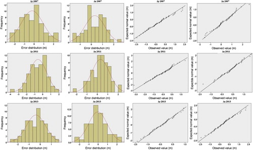
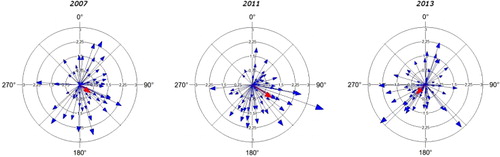
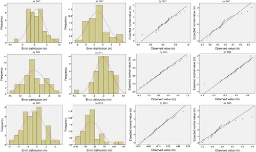
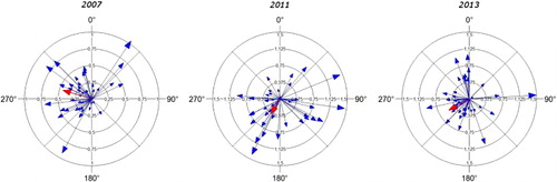
Descriptive statistics of positional error values for PFs and GPSs of the three GE images along East (Δx) and North (Δy) axes are reported in Tables 1 and 2, respectively. The values for normality tests like skewness and kurtosis, K-S test, and the S-W test, used as a goodness of fit statistic for the null hypothesis of normal distribution, are reported in Tables 3 and 4 for PFs and GPSs, respectively. The distribution plots (histogram and quantile-quantile Q-Q plot) of errors for each of the three images along East and North axes for PFs and GPSs are visualized in Figures 5 and 7, respectively. Figures 6 and 8 depict azimuthal direction of errors for PFs and GPSs, respectively. Histograms provide a first indication of the normality of the error distribution, while Q-Q plot (quantiles of empirical data against the ideal) gives a better diagnostic for checking a deviation from the normal distribution (Höhle and Höhle 2009).

Table 1. Statistical differences between PFs and the respective points for the three GE images.

	GE07 – PF		GE11 – PF		GE13 – PF
Basic statistics	Δx (m)	Δy (m)	Δx (m)	Δy (m)	Δx (m)	Δy (m)
Mean	0.31	−0.20	0.31	−0.58	−0.03	−0.38
Min/max	−1.54/+2.62	−2.46/+2.29	−2.21/+2.14	−3.72/+1.95	−2.44/+2.23	−2.36/+1.38
SD	0.87	1.12	0.85	1.07	0.99	0.85
Standard error	0.12	0.15	0.11	0.14	0.13	0.11
CI	0.23	0.3	0.23	0.28	0.26	0.22
RMSE	0.92	1.13	0.9	1.2	0.98	0.93
RMSE (Δxy)	1.45		1.51		1.35
NSSDA (CL95)	2.51		2.57		2.34
Azimuths mean direction	125.9°		123.4°		224.1°

Note: Sample size 57. Δx: Easting error; Δy: Northing error; Min: minimum; Max: maximum; SD: standard deviation; CI: confidence interval for SD (95%); CL95: confidence level 95%.

Table 2. Statistical differences between GPSs and the respective points for the three GE images.

	GE07 – GPS		GE11 – GPS		GE13 – GPS
Basic statistics	Δx (m)	Δy (m)	Δx (m)	Δy (m)	Δx (m)	Δy (m)
Mean	−0.16	0.08	−0.01	−0.27	−0.17	−0.09
Min/max	−0.7/+0.58	−0.81/+0.87	−1.41/+0.64	−1.41/+0.94	−1.00/+0.66	−0.70/+0.6
SD	0.28	0.30	0.42	0.55	0.48	0.28
Standard error	0.04	0.05	0.06	0.09	0.07	0.04
CI	0.09	0.09	0.14	0.17	0.15	0.09
RMSE	0.32	0.31	0.42	0.61	0.51	0.29
RMSE (Δxy)	0.45		0.65		0.52
NSSDA (CL95)	0.77		1.26		0.91
Azimuths mean direction	287.1°		211.8°		241.6°

Note: Sample size 41; 39 samples for GE13. Δx: Easting error; Δy: Northing error; Min: minimum; Max: maximum; SD: standard deviation; CI: confidence interval for SD (95%); CL95: confidence level 95%.

Table 3. Normality testing of PFs positional errors for the three GE images.

	GE07 – PF		GE11 – PF		GE13 – PF
Normality test	Δx	Δy	Δx	Δy	Δx	Δy
Skewness	−0.090	0.270	−0.36	−0.34	0.136	−0.058
Kurtosis	−0.001	−0.262	0.36	0.32	0.112	−0.412
K-S*	0.068 (sig. 0.200)	0.070 (sig. 0.200)	0.099 (sig. 0.200)	0.077 (sig. 0.200)	0.068 (sig. 0.200)	0.060 (sig. 0.200)
S-W	0.980 (sig. 0.463)	0.982 (sig. 0.548)	0.983 (sig. 0.620)	0.984 (sig. 0.640)	0.990 (sig. 0.912)	0.989 (sig. 0.887)

Note: Sample size 57. Δx: Easting error; Δy: Northing error; sig.: significant at p < .05.

*Lilliefors significance correction.

Table 4. Normality testing of GPSs positional errors for the three GE images.

	GE07 – GPS		GE11 – GPS		GE13 – GPS
Normality test	Δx	Δy	Δx	Δy	Δx	Δy
Skewness	0.746	0.038	−0.825	0.129	0.149	0.212
Kurtosis	0.660	1.375	1.575	−0.398	0.436	0.020
K-S*	0.139 (sig. 0.05)	0.120 (sig. 0.146)	0.081 (sig. 0.200)	0.075 (sig. 0.200)	0.181 (sig. 0.135)	0.068 (sig. 0.200)
S-W	0.946 (sig. 0.053)	0.960 (sig. 0.153)	0.953 (sig. 0.089)	0.990 (sig. 0.972)	0.972 (sig. 0.422)	0.989 (sig. 0.956)

Note: Sample size 41; 39 samples for GE13. Δx: Easting error; Δy: Northing error; sig.: significant at p < .05.

*Lilliefors significance correction.

Figure 5. PF CP error frequencies and normal Q-Q plot for the distributions Δx and Δy. Superimposed curve in the histogram represents the normal distribution.

Figure 6. Circular statistics of PF CPs azimuth vectors error. The blue arrows show the topographical direction of the vectors (0°/North clockwise), and the red arrow shows the mean direction of the vectors.

Figure 7. GPS CP error frequencies and normal Q-Q plot for the distributions Δx and Δy. Superimposed curve in the histogram represents the normal distribution.

Figure 8. Circular statistics of GPS CPs azimuth vectors error. The blue arrow shows the topographical direction of the vectors (0°/North clockwise), and the red arrow shows the mean direction of the vectors.

3.1.1. PF points

The histograms of GE07, GE11, and GE13 reveal that the superimposed curves for a normal distribution (Gaussian bell curve) does not match the data very well along East and North component, with deviations from the sharper peak around the mean and relative less for the tails. These distributions tend to have a peak in the center of the distribution and seem leptokurtic. Nevertheless, the detrended Q-Q plot for both East and North components follows a normal distribution (straight line) with the exception of few outliers at the end of positive values, especially for East distribution in all three images.

The mean values (Table 1) lower than the standard deviations denote a fairly tight dispersion in the data and the absence of systematic errors (Aguilar, Aguilar, and Agüera 2007), while the coefficients of skewness and kurtosis gave values lower than ±0.5 (Table 3) and can be considered to be close to those of a normal distribution (Daniel and Tennant 2001; Höhle and Höhle 2009). In addition, K-S test statistics ranges from 0.060 to 0.099 and the p-values (significance) are all .200, while S-W test ranges from 0.980 to 0.990 while the p-values (significance) range from .463 to .912. The predefined significance level is 0.05, and thus do not reject the null hypothesis that data violate the normal distribution. As shown in the Table 1, the NSSDA horizontal accuracy of the data-set reveals quite similar values, with the best value for the GE13 (RMSE_CL95 = 2.34 m), followed by GE07 (RMSE_CL95 = 2.51 m), than GE11 (RMSE_CL95 = 2.57 m). Table 1 also reveals that the East and North RMSE component are similar but not identical. The low standard deviations (Δy GE13 = 0.85 m and Δx GE11 = 0.85 m up to Δy GE13 = 1.24 m) reflect the good geometric stability of the images data-set. The minimum and maximum Δx error values (−2.44 m and 2.62 m) appear on GE13 and GE07, respectively, while both the minimum and maximum Δy error values (−3.72 m and 2.29 m) appear on GE11 and GE07, respectively. The plots of vector errors shown in Figure 6 provide another interesting point of view, revealing in which direction the error dominates. The mean direction value was 125.9° in GE07, 123.4° in GE11, and 224.1° in GE13. The overall errors were quite randomly distributed; nonetheless, the azimuthal errors in the image GE11 are more concentrated toward South-East.

3.1.2. GPS points

The histograms of GE07, GE11, and GE13 show that the superimposed curves for a normal distribution match the data quite well along East and North component, with little deviations from the sharper peak around the mean. These distributions tend to have peaks in the center of the distribution and seems leptokurtic. In addition, the detrended Q-Q plot for both East and North components follows a normal distribution with the exception of few outliers at the end of positive values, especially for East distribution in all three images.

While the mean values and standard deviations (Table 2) are still similar to those observed in PFs points, denoting a fairly tight dispersion in the data, interestingly the coefficients of skewness and kurtosis gave some outliers higher than ±0.5. In fact, two outliers of GE13 were deleted since exceeded the maximum tolerable discrepancy, applied to identify blunder errors in the data-set. These outliers can also be seen in Q-Q plot from GE13 (Figure 7), where points at the right end of plot are further away from the line than elsewhere. The concept of maximum tolerable discrepancy is defined as three times the calculated RMSE (Kapnias, Milenov, and Kay 2008). The results obtained from the K-S test reported in Table 4 range from 0.075 to 0.139 and the p-values range from .050 to .200, while S-W test ranges from 0.946 to 0.990 while the p-values range from .053 to .972. These results are nonsignificant at the p-value = .05 and imply that the data-set is approximately normally distributed. The NSSDA horizontal accuracy from GPSs resulted in the lowest values compared with the PFs (Table 2), with the best result for the GE07 (RMSE_CL95 = 0.77 m), followed by GE13 (RMSE_CL95 = 1.00 m), than GE11 (RMSE_CL95 = 1.26 m). Overall, the East and North RMSE components are similar but not identical, with lowest values compared with the PFs. The low standard deviations (Δy GE13= 0.28 m, Δx GE07= 0.28 m up to Δy GE11= 0.55 m) reflect the high geometric stability of the images data-set. The minimum and maximum Δx error values (−1.41 m and 0.66 m) appear on GE11 and GE13, respectively, while both the minimum and maximum Δy error values (−1.41 m and 0.94 m) appear on GE11. Figure 8 reveals that the plots of vector errors are quite randomly distributed, except the azimuthal errors in the image GE07 that are more concentrated toward Northeastern quadrant. The mean direction value was 287.1° in GE07, 211.8° in GE11, and 241.6° in GE13.

4. Discussion

One of the main goals of this study was to assess horizontal accuracy of GE images in the city of Rome. Prior studies have been undertaken at both the global and regional scales to accomplish this goal by using and testing different CPs. For instance, at a global scale Potere (2008) estimated a positional accuracy of 39.7 m RMSE_r, collecting CPs extracted from the Landsat GeoCover, while Yousefzadeh and Mojaradi (2012) estimated horizontal accuracy in 6.1 m RMSE_r, by using CPs extracted from 1:2000 scale maps of three towns of the study area in Iran. In another major study, Paredes-Hernandez et al. (2013) have recently reported an accuracy of 5.0 m RMSE_r, by using CPs located over a rural area and extracted from a cadastral database. As expected, the results obtained in this study also gave different accuracies for the two different sets of CPs and suggest that the horizontal accuracy estimated using inferred GPS points is higher than the accuracy estimated using only PF points (Tables 1–2). Overall, taking into account the resolution of the images, our results indicate the submeter accuracy for the images GE07 and GE13, while GE11 shows an accuracy slightly higher than 1 m. Besides, the image GE11 has a lower accuracy in both tests and almost always shows high error values of the minimum and maximum Δx and Δy. A possible explanation for these results may be the use of inaccurate Digital Elevation Model (DEM) used through the orthorectification process. In fact, the accuracy of the images is heavily dependent upon the accuracy of the orientation data plus the quality of DEM used (Toutin 2004; Aguilar et al. 2012). Unfortunately, as pointed out by Potere (2008) we could not assess how much of these differences in accuracies was due to DEM effects, since Google Inc. do not release details of the processing chain by its data provider. Nevertheless, these findings are consistent with those of earlier studies, which showed that the accuracy increases by using more accurate CP datasets. Despite the fact that field measurements with total station are generally more precise than GPS points, another possible explanation is that PFs were initially represented in the local Cassini-Soldner projection, and then transformed into WGS-84. Thus, this transformation may have introduced a systematic error greater than 1 m. This finding is in agreement with Dardanelli, Franco, and Catalano (2011), who performed a GPS survey to evaluate the accuracy of PF points in urban environment, obtaining values consistent with our results (i.e. GPSs residual errors: ±1 m, PFs residual errors: ±2 m), supporting the robustness of the data-set. In any case, the use of PF points can be an interesting reference database to evaluate the accuracy of images at medium and low resolution. Whereas NSSDA assumes that systematic errors should be eliminated as best as possible, histograms, Q-Q plots, estimation of azimuthal errors, and statistical tests are further computed to disclose nonnormality in the data. Overall, the more robust choice to check if the data follow a normal distribution is a statistical test. A number of authors have reported the use of K-S and S-W tests as a goodness of fit to test for the normality and uniformity of the data for the analysis of errors in the positional accuracy of images (Zandbergen 2008; Cuartero et al. 2010; Aguilar, del Mar Saldaña, and Aguilar 2013). In particular, the S-W test has become the most preferred normality test because of its powerful properties in the range 3 ≤ n ≤ 5000 (Yazici and Yolacan 2007; Razali and Wah 2011). For example, Yap and Sim (2011) argue that the S-W test has good power properties over a wide range of asymmetric distributions, symmetric with low kurtosis values and symmetric distribution with high sample kurtosis. In our case, the results of the K-S and S-W tests gave a p-value that supports a decision to accept the null hypothesis of normal distribution. The p-value is an estimate of the probability that a random sample would generate data that deviate from the normal distribution as much as the observed data do. More specifically, the p-value provides an assessment of the compatibility of the data with the null hypothesis, not the probability that the null hypothesis is correct. Since our p-values are greater than our α-level (i.e. 0.05), we do not reject the assumption and conclude that these data do not violate the null hypothesis. These findings are not really unexpected. Positional errors of spatial data (both horizontal and vertical) are spatially dependent, tend to be positively autocorrelated (Goodchild 2009), and generally are not normally distributed. Overall, greater positional uncertainty is associated with rugged terrain (Beekhuizen et al. 2011), while vertical error increased with surface slope (Pulighe and Fava 2013). However, it seems possible that the flat relief of the study area may have reduced outliers and sources of error involved in sampling, as well as an improved orthorectification procedure of the images analyzed. Several studies have revealed that inappropriate DEM with poor grid resolution can generate artifacts (e.g. wiggly roads or edges) with high-resolution images, especially over high-relief study site (Zhang, Tao, and Mercer 2001; Toutin 2004). With regard to outliers observed in the histogram from the image GE13, for the purposes of the accuracy assessment performed in this paper, there is no theoretical reason to assume that the omission of these affect the results, since the number of CPs used is sufficiently large to achieve a certain confidence level. Regarding the presence of systematic errors, the distributions of the errors of PF points (Figure 7) do not show apparent patterns in the direction East and North, except the azimuthal errors in the image GE11 that are more concentrated toward South-East. Likewise, the distribution of the errors of GPS points (Figure 8) suggests that error vectors are randomly distributed, except the azimuthal errors in the image GE07, which are more concentrated toward North-West. A possible explanation for these findings might be the aforementioned DEM impact. We stress the importance of the accurate orthorectification process (Tong, Liu, and Weng 2010; Aguilar, del Mar Saldaña, and Aguilar 2013). One of the most important findings that has emerged from the research is that GE’s imagery in the city of Rome constitutes a suitable source of information for scientific research and other projects, with relative horizontal accuracy fulfilling the RMSE_r requirement of the ASPRS (2013) for the production of 1:2000 (GE07 and GE13) or 1:2500 topographic maps (GE11).

5. Conclusion

The research described in this paper addresses an assessment of the horizontal accuracy of GE images (Rome, Italy) for the years 2007, 2011, and 2013, based on the use of GPS points and cadastral points as independent reference control data. Data quality evaluation procedure follows the methodology of the NSSDA set up by the US Federal Geographic Data Committee, which compute horizontal (radial) accuracy at the 95% confidence level. According to the results achieved, it is possible to state that GE’s VHR imageries of Rome have an overall positional accuracy close to 1 m that is sufficient for deriving very accurate ground truth samples and measurements and suitable for the production of large-scale planimetric maps. Assessing the accuracy of these images is an essential step toward using the data-set for academic research purposes, relevant also to the topic of DE. However, we emphasize the fact that our results are limited to the high-resolution images of Rome study area, where particular attention was paid when defining the study area and the boundaries of the image mosaic. Although this work is focused on images in urban area, since GE is a global imagery mosaic, the described approach could be applied also in study areas with high-resolution imagery in many parts of the world. Future research should concentrate on the investigation of accuracy assessment on areas of complex topography, as well as forests and mountain areas.

Disclosure statement

No potential conflict of interest was reported by the authors.

Additional information

Funding

This research was partially funded by the Italian Ministry of Agricultural Policies under the Istituto Nazionale di Economia Agraria project ‘Promozione della Cultura Contadina’ (http://www.inea.it/cultura-contadina).

References

- Aguilar, F. J., M. A. Aguilar, and F. Agüera. 2007. “Accuracy Assessment of Digital Elevation Models Using a Non-parametric Approach.” International Journal of Geographical Information Science 21: 667–686. doi:10.1080/13658810601079783.
- Aguilar, M. A., F. J. Aguilar, M. del Mar Saldaña, and I. Fernández. 2012. “Geopositioning Accuracy Assessment of GeoEye-1 Panchromatic and Multispectral Imagery.” Photogrammetric Engineering & Remote Sensing 78 (3): 247–257. doi:10.14358/PERS.78.3.247.
- Aguilar, M. A., M. del Mar Saldaña, and F. J. Aguilar. 2013. “Assessing Geometric Accuracy of the Orthorectification Process from GeoEye-1 and WorldView-2 Panchromatic Images.” International Journal of Applied Earth Observation and Geoinformation 21: 427–435. doi:10.1016/j.jag.2012.06.004.
- Al-Abdulrazzak, D., and D. Pauly. 2013. “Managing Fisheries from Space: Google Earth Improves Estimates of Distant Fish Catches.” ICES Journal of Marine Science 71: 450–454. doi:10.1093/icesjms/fst178.
- Ariza, F. J., and A. D. J. Atkinson. 2005. “Sample Size and Confidence When Applying the NSSDA.” Proceedings of the 21th International Cartographic Conference, The International Cartographic Association, La Coruña, Spain, July 9–16.
- ASPRS. 1990. “American Society for Photogrammetry and Remote Sensing. ASPRS accuracy standards for large-scale maps.” Photogrammetric Engineering and Remote Sensing 56: 1068–1070.
- ASPRS. 2013. “American Society for Photogrammetry and Remote Sensing. ASPRS accuracy standards for digital geospatial data.” Photogrammetric Engineering & Remote Sensing 79 (12): 1073–1085.
- Barbarella, M. 2014. “Digital Technology and Geodetic Infrastructures in Italian Cartography.” Città e Storia IX (1): 91–110. Università Roma Tre-CROMA.
- Beekhuizen, J., G. B. M. Heuvelink, J. Biesemans, and I. Reusen. 2011. “Effect of DEM Uncertainty on the Positional Accuracy of Airborne Imagery.” IEEE Transactions on Geoscience and Remote Sensing V49 (5): 156–172. doi:10.1109/TGRS.2010.208367.
- Benham, P. M., E. J. Beckman, S. G. DuBay, L. M. Flores, A. B. Johnson, M. J. Lelevier, C. J. Schmitt, N. A. Wright, and C. C. Witt. 2011. “Satellite Imagery Reveals New Critical Habitat for Endangered Bird Species in the High Andes of Peru.” Endangered Species Research 13 (2): 145–157. doi:10.3354/esr00323.
- Chang, A. Y., M. E. Parrales, J. Jimenez, M. E. Sobieszczyk, S. M. Hammer, D. J. Copenhaver, and R. P. Kulkarni. 2009. “Combining Google Earth and GIS Mapping Technologies in a Dengue Surveillance System for Developing Countries.” International Journal of Health Geographics 8 (1): 49. doi:10.1186/1476-072X-8-49.
- Chen, A., G. Leptoukh, S. Kempler, C. Lynnes, A. Savtchenko, D. Nadeau, and J. Farley. 2009. “Visualization of A-train Vertical Profiles Using Google Earth.” Computers & Geosciences 35: 419–427. http://dx.doi.org/10.1016/j.cageo.2008.08.006.
- Congalton, R. G., and K. Green. 2009. Assessing the Accuracy of Remote Sensing Data. 2nd ed. Boca Raton, FL: CRC Press, 208 p.
- Contreras, D.A., and N. Brodie. 2010. “Quantifying Destruction: An Evaluation of the Utility of Publicly-available Satellite Imagery for Investigating Looting of Archaeological Sites in Jordan.” Journal of Field Archaeology 35 (1): 101–114. doi:10.1179/009346910X12707320296838.
- Cracknell, A. P., K. D. Kanniah, K. P. Tan, and L. Wang. 2013. “Evaluation of MODIS Gross Primary Productivity and Land Cover Products for the Humid Tropics Using Oil Palm Trees in Peninsular Malaysia and Google Earth Imagery.” International Journal of Remote Sensing 34: 7400–7423. doi:10.1080/01431161.2013.820367.
- Cuartero, A., A. M. Felicisimo, M. E. Polo, A. Caro, and P. G. Rodriguez. 2010. “Positional Accuracy Analysis of Satellite Imagery by Circular Statistics.” Photogrammetric Engineering and Remote Sensing 76: 1275–1286. doi:10.14358/PERS.76.11.1275.
- Daniel, C., and K. Tennant. 2001. “DEM Quality Assessment.” In Digital Elevation Model Technologies and Applications: The DEM User Manual, 1st ed., edited by D. F. Maune, 395–440.
- Dardanelli, G., V. Franco, and S. Catalano. 2011. “Analisi cartografica e GPS di punti fiduciali.” Atti 15 a Conferenza Nazionale ASITA – Reggia di Colorno, 15–18Novembre 2011 (In Italian). Accessed June 15. http://www.attiasita.it/ASITA2011/Pdf/043.pdf.
- Dong, J., X. Xiao, S. Sheldon, C. Biradar, N. D. Duong, and M. Hazarika. 2012. “A Comparison of Forest Cover Maps in Mainland Southeast Asia from Multiple Sources: PALSAR, MERIS, MODIS and FRA.” Remote Sensing of Environment 127: 60–73. doi:10.1016/j.rse.2012.08.022.
- Dorais, A., and J. Cardille. 2011. “Strategies for Incorporating High-Resolution Google Earth Databases to Guide and Validate Classifications: Understanding Deforestation in Borneo.” Remote Sensing 3: 1157–1176. doi:10.3390/rs3061157.
- FGDC. 1998. Geospatial Positioning Accuracy Standards. Part 3: National Standard for Spatial Data Accuracy. Virginia: Federal Geographic Data Committee Reston.
- Fisher, G. B., C. B. Amos, B. Bookhagen, D. W. Burbank, and V. Godard. 2012. “Channel Widths, Landslides, Faults, and Beyond: The New World Order of High Spatial Resolution Google Earth Imagery in the Study of Earth Surface Processes.” In Google Earth and Virtual Visualizations in Geoscience Education and Research, edited by S. J. Whitmeyer, J. E. Bailey, D. G. De Paor, and T. Ornduff, 1–22. Geological Society of America Special Paper 492. doi:10.1130/2012.2492(01).
- Frankl, A., A. Zwertvaegher, J. Poesen, and J. Nyssen. 2013. “Transferring Google Earth Observations to GIS-software: Example from Gully Erosion Study.” International Journal of Digital Earth 6 (2): 196–201. doi:http://dx.doi.org/10.1080/17538947.2012.744777.
- Goodchild, M. F. 2009. “The Quality of Geospatial Context.” In QuaCon 2009, 15–24. LNCS, Volume 5786. Heidelberg: Springer.
- Goodchild, M. F., H. Guo, A. Annoni, L. Bian, K. de Bie, F. Campbell, M. Craglia, et al. 2012. “Next-generation Digital Earth.” Proceedings of the National Academy of Sciences 109: 11088–11094. doi:10.1073/pnas.120238310.
- Goodchild, M. F., and G. J. Hunter. 1997. “A Simple Positional Accuracy Measure for Linear Features.” International Journal of Geographical Information Systems 11: 299–306. doi:10.1080/136588197242419.
- Höhle, J., and M. Höhle. 2009. “Accuracy Assessment of Digital Elevation Models by Means of Robust Statistical Methods.” ISPRS Journal of Photogrammetry and Remote Sensing 64: 398–406. doi:10.1016/j.isprsjprs.2009.02.003.
- Kapnias, D., P. Milenov, and S. Kay. 2008. Guidelines for Best Practice and Quality Checking of Ortho Imagery, Issue 3.0. Ispra, VA: European Commission Joint Research Centre Institute for the Protection and Security of the Citizen. doi:10.2788/36028.
- Lin, H., F. R. Huang, and G. N. Lu. 2009. “Development of Virtual Geographic Environments and the New Initiative in Experimental Geography”. Acta Geographica Sinica 64 (1): 7–20.
- Marais, J., and B. Godefroy. 2006. “Analysis and Optimal Use of GNSS Pseudo-range Delays in Urban Canyons.” Proceedings of IEEE Computational Engineering in Systems Applications (CESA), Beijing, October 4–6. doi:10.1109/CESA.2006.4281619.
- McRoberts, R. E. 2010. “The Effects of Rectification and Global Positioning System Errors on Satellite Image-based Estimates of Forest Area.” Remote Sensing of Environment 114: 1710–1717. http://dx.doi.org/10.1016/j.rse.2010.03.001.
- Nornadiah, M. R., and B. W. Yap. 2011. “Power Comparison of Shapiro-Wilk, Kolmogorov-Smirnov, Lilliefors and Anderson Darling Tests.” Journal of Statistical Modeling and Analytics 2 (1): 21–33.
- Paredes-Hernandez, C. U, W. E. Salinas-Castillo, F. Guevara-Cortina, and X. Martinez-Becerra. 2013. “Horizontal Positional Accuracy of Google Earth’s Imagery over Rural Areas: A Study Case in Tamaulipas, Mexico.” Boletim de Ciências Geodésicas 19: 588–601. http://dx.doi.org/10.1590/S1982-21702013000400005.
- Ploton, P., R. Pélissier, C. Proisy, T. Flavenot, N. Barbier, S. N. Rai, and P. Couteron. 2012. “Assessing Aboveground Tropical Forest Biomass Using Google Earth Canopy Images.” Ecological Applications 22: 993–1003. http://dx.doi.org/10.1890/11-1606.1.
- Potere, D. 2008. “Horizontal Positional Accuracy of Google Earth’s High-resolution Imagery Archive.” Sensors 8: 7973–7981. doi:10.3390/s8127973.
- Potere, D., A. Schneider, S. Angel, and D. L. Civco. 2009. “Mapping Urban Areas on a Global Scale: Which of the Eight Maps Now Available Is More Accurate?” International Journal of Remote Sensing 30: 6531–6558. doi:10.1080/01431160903121134.
- Pulighe, G., and F. Fava. 2013. “DEM Extraction from Archive Aerial Photos: Accuracy Assessment in Areas of Complex Topography.” European Journal of Remote Sensing 46: 363–378. doi:10.5721/EuJRS20134621.
- Razali, N. M., and Y. B. Wah. 2011. “Power Comparisons of Shapiro-Wilk, Kolmogorov-Smirnov, Lilliefors and Anderson-Darling Tests.” Journal of Statistical Modeling and Analytics 2 (1): 21–33.
- Reimann, C., P. Filzmoser, R. G. Garrett, and R. Dutter. 2008. Statistical Data Analysis Explained: Applied Environmental Statistics. Chichester: John Wiley & Sons.
- Sato, H. P., and E. L. Harp. 2009. “Interpretation of Earthquake-induced Landslides Triggered by the 12 May 2008, M7.9 Wenchuan Earthquake in the Beichuan Area, Sichuan Province, China Using Satellite Imagery and Google Earth.” Landslides 6 (2): 153–159. doi:10.1007/s10346-009-0147-6.
- She, J., Y. Zhang, X. Li, and Y. Chen. 2014. “Changes in Snow and Glacier Cover in an Arid Watershed of the Western Kunlun Mountains Using Multisource Remote-sensing Data.” International Journal of Remote Sensing 35 (1): 234–252. doi:10.1080/01431161.2013.866296.
- Taylor, J. R., and S. T. Lovell. 2012. “Mapping Public and Private Spaces of Urban Agriculture in Chicago through the Analysis of High-resolution Aerial Images in Google Earth.” Landscape and Urban Planning 108 (1): 57–70. doi:10.1016/j.landurbplan.2012.08.001.
- Tong, X., S. Liu, and Q. Weng. 2010. “Bias-corrected Rational Polynomial Coefficients for High Accuracy Geo-positioning of QuickBird Stereo Imagery.” ISPRS Journal of Photogrammetry and Remote Sensing 65 (2): 218–226. doi:10.1016/j.isprsjprs.2009.12.004.
- Toutin, T. 2004. “Review Paper: Geometric Processing of Remote Sensing Images: Models, Algorithms and Methods.” International Journal of Remote Sensing 25 (10): 1893–1924. doi:10.1080/0143116031000101611.
- Wang Y., G. Huynh, and C. Williamson. 2013. “Integration of Google Maps/Earth with Microscale Meteorology Models and Data Visualization.” Computers & Geosciences 61: 23–31. doi:10.1016/j.bbr.2011.03.031.
- Yamagishi, Y., H. Yanaka, K. Suzuki, S. Tsuboi, T. Isse, M. Obayashi, H. Tamura, and H. Nagao. 2010. “Visualization of Geoscience Data on Google Earth: Development of a Data Converter System for Seismic Tomographic Models.” Computers & Geosciences 36 (3): 373–382. doi:10.1016/j.cageo.2009.08.007.
- Yap, B. W., C. H. Sim. 2011. “Comparisons of Various Types of Normality Tests.” Journal of Statistical Computation and Simulation 81: 2141–2155. doi:10.1080/00949655.2010.520163.
- Yazici, B., and S. Yolacan. 2007. “A Comparison of Various Tests of Normality.” Journal of Statistical Computation and Simulation 77 (2): 175–183. doi:10.1080/10629360600678310.
- Yousefzadeh, M., and B. Mojaradi. 2012. “Combined Rigorous-generic Direct Orthorectification Procedure for IRS-p6 Sensors.” ISPRS Journal of Photogrammetry and Remote Sensing 74: 122–132. http://dx.doi.org/10.1016/j.bbr.2011.03.031.
- Yu, L., and P. Gong. 2012. “Google Earth as a Virtual Globe Tool for Earth Science Applications at the Global Scale: Progress and Perspectives.” International Journal of Remote Sensing 33: 3966–3986. doi:10.1080/01431161.2011.636081.
- Zandbergen, P. A. 2008. “Positional Accuracy of Spatial Data: Non-Normal Distributions and a Critique of the National Standard for Spatial Data Accuracy.” Transactions in GIS 12 (1): 103–130. doi:10.1111/j.1467-9671.2008.01088.x.
- Zhang, Y., V. Tao, and B. Mercer. 2001. “Assessment of the Influences of Satellite Viewing Angle, Earth Curvature, Relief Height, Geographical Location and DEM Characteristics on Planimetric Displacement of High-resolution Satellite Imagery.” Proceedings of the ASPRS Annual Conference, St Louis, Missouri, April 23–27 (CD-ROM, unpaginated).