Mapping floods due to Hurricane Sandy using NPP VIIRS and ATMS data and geotagged Flickr imagery

Abstract

In this study, we present an approach to estimate the extent of large-scale coastal floods caused by Hurricane Sandy using passive optical and microwave remote sensing data. The approach estimates the water fraction from coarse-resolution VIIRS and ATMS data through mixed-pixel linear decomposition. Based on the water fraction difference, using the physical characteristics of water inundation in a basin, the flood map derived from the coarse-resolution VIIRS and ATMS measurements was extrapolated to a higher spatial resolution of 30 m using topographic information. It is found that flood map derived from VIIRS shows less inundated area than the Federal Emergency Management Agency (FEMA) flood map and the ground observations. The bias was mainly caused by the time difference in observations. This is because VIIRS can only detect flood under clear conditions, while we can only find some clear-sky data around the New York area on 4 November 2012, when most flooding water already receded. Meanwhile, microwave measurements can penetrate through clouds and sense surface water bodies under clear-or-cloudy conditions. We therefore developed a new method to derive flood maps from passive microwave ATMS observations. To evaluate the flood mapping method, the corresponding ground observations and the FEMA storm surge flooding (SSF) products are used. The results show there was good agreement between our ATMS and the FEMA SSF flood areas, with a correlation of 0.95. Furthermore, we compared our results to geotagged Flickr contributions reporting flooding, and found that 95% of these Flickr reports were distributed within the ATMS-derived flood area, supporting the argument that such crowd-generated content can be valuable for remote sensing operations. Overall, the methodology presented in this paper was able to produce high-quality and high-resolution flood maps over large-scale coastal areas.

Keywords:

• coastal flood
• hurricane
• water fraction
• high-resolution flood mapping
• VIIRS
• ATMS

1. Introduction

Coastal floods induced by hurricane storm surge are some of the frequent, costly, and deadly hazards that can affect coastal communities. Hurricane Sandy, the largest Atlantic hurricane on record, devastated portions of the Mid-Atlantic and Northeastern USA in late October 2012. Preliminary estimates of losses that include business interruption surpass $50 billion (2012 USD).

Rapid assessment of the spatial extent of large-scale flooding event is highly important for relief and rescue operations, and satellite remote sensing is eminently suitable for this task (Sheng, Gong, and Xiao 2001; Sun, Yu, and Goldberg 2011; Sun et al. 2012). Under clear conditions during daytime, flood maps can be derived from optical sensors, such as visible, near-infrared (Sheng, Gong, and Xiao 2001; Sun, Yu, and Goldberg 2011; Sun et al. 2012), and shortwave-infrared (SWIR) observations (Li et al. 2013a). Microwave sensors, including active airborne synthetic aperture radar imagery (Bates et al. 2006), and passive microwave instruments (Sippel et al. 1994; Jin 1999; Tanaka et al. 2003; Zheng et al. 2008), can penetrate through clouds and sense surface water bodies. Compared to active microwave sensors, passive microwave instruments can provide observations at high temporal resolutions; therefore, these data have great potential for estimating large-scale floods, particularly under cloudy conditions that are typically associated with flooding. However, the coarse spatial resolution of these passive microwave sensors may limit their broad application.

In this study, we present an assessment of the effectiveness of passive optical and microwave remote sensing data for flood monitoring, using the aftermath of Hurricane Sandy as a test case. We derive flooding information from NPP VIIRS 375-m imager data and microwave ATMS data, and enhanced our results to a 30-m resolution using the Shuttle Radar Topography Mission (SRTM) digital elevation model (DEM) data. Our results are assessed in comparison of Federal Emergency Management Agency (FEMA) flood map and ground observations to demonstrate the great potential of these sensors for flood monitoring. Furthermore, in this study compared the locations of geotagged Flickr imagery depicting flooding to the flood maps as they were derived through our approach. In our case study, 95% of those geotagged Flickr contributions originated from within the flooded area (as it was mapped through our WFHF method), which indicates that such citizen contributions have merit for assessing the impact areas of natural disasters.

2. Data used

To estimate the coastal flooding due to Hurricane Sandy, the data used are listed as follows:

1. The NPP VIIRS data (Table 1) were obtained from NOAA’s Comprehensive Large Array-data Stewardship Systems (CLASS).

2. The ATMS antenna temperature data records were obtained from NOAA’s CLASS (Weng, Yang, and Zou 2013). Brightness temperatures and satellite zenith angles were extracted from the ATMS HDF5 files. These data were then re-projected into the WGS84 system and re-sampled to 15 × 15 km spatial resolution. The channels shown in Table 2 can be used to observe the Earth’s surface.

3. DEM data from SRTM.

4. River basin boundary data, distributed by the US Geological Survey (USGS), were used to obtain water fraction statistics for high-resolution flood mapping. To construct the mixed pixels along the coastline, the coastline on the river basin boundary was buffered toward the ocean.

5. Land cover data, acquired from the National Land Cover Database 2006 of USGS, were used to obtain pure end-member data and to extract background water information.

6. Linear hydrographic features (major rivers, streams, and canals) and area hydrographic features (major lakes and reservoirs) were used for estimating river density and for deriving pure land end-member data.

7. Three-meter-resolution Hurricane Sandy storm surge flooding (SSF) products generated from field-verified high-water marks (HWM) and storm surge sensor data and distributed by the FEMA were used to evaluate the ATMS-derived flood map. The SSF products were created from the HWMs and storm surge sensor data from the USGS. The HWMs and storm surge sensor data are used to interpolate the water surface elevation; then, the water elevation data are subtracted from the best available DEM to create a depth grid and surge boundary.

8. Ground-level crowd-generated social media reports of floods, in the form of geotagged Flickr imagery, as a complementary source of information, to be contrasted to the satellite-derived flood map.

Table 1. NPP/VIIRS imager multispectral channels used to observe the surface water.

Band no.	Central wavelength (μm)	Wavelength range (µm)	Horizontal sample interval (km)
I1	0.640	0.600–0.680	0.371 × 0.387
I2	0.865	0.846–0.885	0.371 × 0.387
I3	1.61	1.580–1.640	0.371 × 0.387
I5	11.45	10.500–12.400	0.371 × 0.387

Table 2. Characteristics of ATMS channels used to observe the Earth’s surface.

Cannel	Center frequency(GHz)	Beam width(°)	Quasi-polarization	Characterization at nadir
1	23.80	5.2	QV	Surface
2	31.40	5.2	QV	Surface
3	50.30	2.2	QH	Surface
4	51.76	2.2	QH	Surface
16	88.20	2.2	QV	Surface

3. Methodology

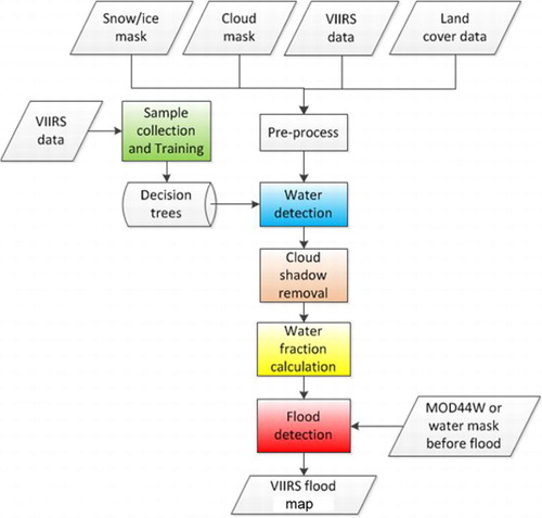
3.1. Derive flooding water fraction from VIIRS under clear conditions

Under clear-sky conditions, a decision tree algorithm will be applied to identify flooded areas (Sun, Yu, and Goldberg 2011; Sun et al. 2012; Li et al. 2013a). Since flood is land inundated by water, flooded pixels are usually water mixed with land. As such, only water fraction can represent this mixed information, so flood map derived from water fraction contains more information than that derived from water classification (Sun, Yu, and Goldberg 2011). Water fraction can be calculated from linear mixture model and a dynamic nearest neighbor searching (DNNS) method developed by Li et al. (2013a):

(1)

By using the characteristic of the VIIRS visible channel I1 (ch1: 0.64 μm), near IR channel I2 (ch2: 0.865 μm) and SWIR channel I3 (ch3: 1.61 μm), the DNNS method can be used to dynamically search the nearby land and water end-members:

(2)

Flooding water fraction can be obtained by the difference in water fraction after and before flood.

3.2. Cloud shadow detection

Another critical component of this technique is a geometric correction method recently developed by Li et al. (2013c) to remove cloud shadows from water detection results (Li et al. 2013c). This is a critical step in flood mapping, as current techniques that rely on optical satellite imagery are severely affected by a large portion of cloud shadow pixels that are misclassified as water. The viability of necessary retrieval methods and new sensor capabilities has been demonstrated for flood detection using Hurricane Sandy, and the recent flood cases in Alaska and Colorado as primary operational test scenarios. The flowchart for deriving water fraction and flood from VIIRS is described in Figure 1.

Figure 1. Flowchart for deriving flood from VIIRS data.

3.3. Inundation model to derive high-resolution flood maps

According to water’s hydrodynamic properties, when flooding occurs, inundated areas are affected sequentially from lowest to the highest point in elevation. If the topography is not very steep around the water bodies, the higher the water level, the larger the inundated area. This inundation mechanism can be expressed as:

(3)

where, A is the total water area between the minimal surface elevation, min_h, and maximal inundated surface elevation, max_h ; and f(h) is the increment of water area with the change of surface elevation h. Equation (3) indicates the relationship between inundated area and surface elevation. Because both the minimal surface elevation, min_h, and the increment function of water area in a specific region, f(h), can be derived from the DEM, the maximal inundated surface elevation, max_h, decides the total water area (Li, Sun, and Yu 2013b). Consequently, the maximal inundated surface elevation, max_h, can also be calculated if the total water area A is known.

Since optical satellite data, such as VIIRS, can only map the land surface under clear-sky conditions when major locations affected by Hurricane Sandy can only be detected four days after the hurricane’s passing (4 November 2012). As shown in Figure 4, by that time, flooding conditions had already receded in most affected regions. The peak floods due to Hurricane Sandy were under cloudy conditions. Accordingly, we developed a new algorithm to derive flood maps from passive microwave data; namely, the ATMS sensor on board the Suomi-NPP, which can penetrate through clouds to observe the surface.

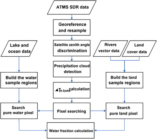
3.4. Deriving flooding water fraction from ATMS under all weather conditions

3.4.1. Precipitating cloud detection

Despite its overall resilience in cloudy conditions, passive microwave signals can still be affected by clouds (Cho and Nishiura 2010). In particular, higher frequency channels cannot penetrate precipitating clouds. Before extracting the surface information, precipitating clouds should be detected and masked. Precipitating clouds can be defined by comparing the brightness temperature at 89 GHz versus 22 GHz, as the former has substantially lower values (Ferraro et al. 1998). Accordingly, we defined a pixel in the ATMS imagery as a cloud-contaminated pixel if it met the following condition:

(4)

where BT₁₆ and BT₁ are the brightness temperatures of channels 16 and 1, respectively, and T_RAIN (10.0) is a threshold value to distinguish precipitation areas from other objects.

3.4.2. Satellite zenith angle limitation

Pixels with large satellite zenith angles have a lower spatial resolution than those near nadir. Accordingly, we chose the pixels with smaller angles to extract related information by removing pixels with satellite zenith angle greater than 50°. Satellite zenith angle data are available in ATMS’s HDF5 file, which provides such information for each ATMS pixel.

3.4.3. Water fraction calculation method

Water body detection and area calculations are key steps for flood estimations. Channels 3 and 4 of the ATMS data have longer wavelengths and better penetrate through clouds than channel 16. Furthermore, these two channels are similarly affected by the atmosphere due to their similar frequencies. Following previous researchers’ use of the polarization difference of 37 GHz (Sippel et al. 1994; Choudhury 1989; Sippel et al. 1998), in this study, the brightness temperature difference (ΔT_(4−3)obs) between channels 4 and 3 was used to identify water and land. To test the sensitivity of ΔT_(4−3)obs to water and land, land and water samples were selected from the ATMS data on 16, 17, 21, 22, 26, 27 October and 1 November according to the land cover.

The spatial resolution of ATMS data is 15 km. At this coarse resolution, the land surface is generally comprised by mixed terrain of water and land. ATMS pixels consist of a combination of different microwave signals generated by the water and the land surface fractions, and can be represented as following:

(5)

(6)

where, ΔT_(4−3)obs is the brightness temperature difference of ATMS channels 3 and 4. ΔT_(4−3)wat and ΔT_(4−3)lan are the brightness temperature difference of channels 3 and 4 for water and land, respectively. f_wat and f_lan represent the fractions of water and land, respectively. According to Equations (5) and (6), we can get:

(7)

(8)

From Equation (7), water fraction f_wat can be derived from the Equation (9):

(9)

Two end elements need to be calibrated: ΔT_(4−3)lan and ΔT_(4−3)wat. The calibration of the ΔT_(4−3)wat is rather straightforward, as it can be derived by analyzing the brightness temperatures measured over the lakes or ocean. ΔT_(4−3)lan is calibrated over some selected pixels, which are chosen based on the ATMS channel characters, DEM data, and river basin boundary data. The calibration of land pixels is more complicated, because land end-members are related to soil moisture, vegetation, soil types, and other physiognomical factors.

To find the pure end-member more accurately, we built pure land sample regions according to the land cover data and river density information. We selected land sample pixels with both low river density and similar land cover types to the coastland. Ocean pixels near the coastline were selected as water sample regions. The flowchart for deriving water fraction from ATMS is shown in Figure 2.

Figure 2. Flowchart of water fraction estimation from ATMS data.

4. Results

4.1. Derivation of high-resolution flood map from VIIRS

Figure 3 (upper) shows a false-color image of the VIIRS instrument over the New York metropolitan area, while Figure 3 (lower) shows the derived water fraction distribution in the same area on 4 November 2012.

Figure 3. VIIRS false-color image (VIIRS 3, 2, 1) at 17:17 (GMT) on 4 November 2012. Dark blue and black correspond to water bodies (upper). VIIRS-derived water fraction for the same period using the Li et al.’s (2013c) algorithm (lower).

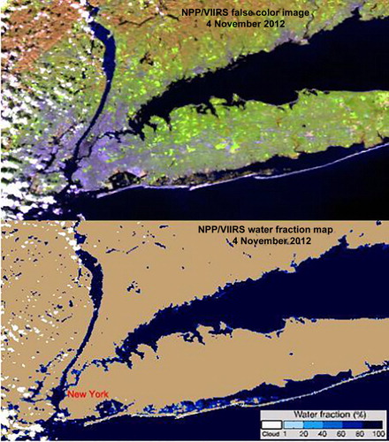
With the water detection result, floodplains can be determined by subtracting water extent before flood. For operational products, we can use water reference map from MODIS Water Mask Product (MOD44W; Carroll et al. 2009) or generate a dynamic reference water map from a composite of water identification map in all clear days during previous month. However, with the original spatial resolution of 375 m of VIIRS, as shown in Figure 3, the flooded area in small regions, like New York, during Hurricane Sandy period, cannot be detected. By applying an inundation model recently developed by Li et al. (2013c) and ingesting DEM data from the SRTM, flood maps derived from VIIRS can be upgraded to 30-m resolution.

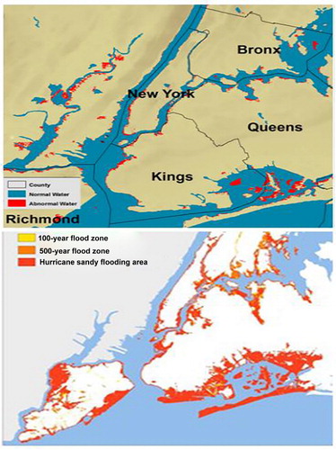
Figure 4 shows a flood map around the New York metropolitan area derived from VIIRS and SRTM 30-m DEM data on 4 November 2012, when only some clear-sky data around the New York area can be found. Compared with flooding zone maps from the FEMA and evacuation estimates during Hurricane Sandy, the VIIRS 30-m flood map on 4 November 2012 shows consistent inundated locations. Nevertheless, the flood map derived from VIIRS shows less inundated area than the FEMA flood map and the ground observations. This is because most flooding water due to Hurricane Sandy already receded on 4 November 2012.

Figure 4. Flood map at 30-m resolution derived from VIIRS and SRTM in the New York metropolitan area on 4 November 2012 (upper) compared with a flooding area map from FEMA over parts of lower Manhattan, the Upper East Side, Red Hook, and Greenpoint (lower).

4.2. Derivation of high-resolution flood map from ATMS

Since microwave instruments, like radar and ATMS, can penetrate through clouds to observe the Earth’s surface, but the radar data are usually very expensive, we therefore developed a new method to derive flood maps from passive microwave ATMS observations.

The water fraction of each ATMS pixel was estimated in accordance with the principle of linear decomposition of mixed pixels. The land and water samples regions generated by river density and land cover data, the relationship of channels 3, 4, and 16, neighborhood pixels searching, and the difference of channels 4 and 3 of ATMS were comprehensively taken into account to dynamically decide the water and land end-members.

Figure 5 shows the resulting water fraction maps derived from the ATMS before and after Hurricane Sandy. With the water detection result at the ATMS coarse resolution (15 km), floodplains can be determined by subtracting water extent before flood. The basin-scale water fraction differences between before and after the flood were calculated to derive flood map, and to reduce the affection of soil moisture and vegetation, avoiding the pixel-to-pixel errors. Figure 5 demonstrates the flood map derived from the ATMS.

Figure 5. Water fraction maps before (left) and after (middle) Hurricane Sandy and their difference map (right).

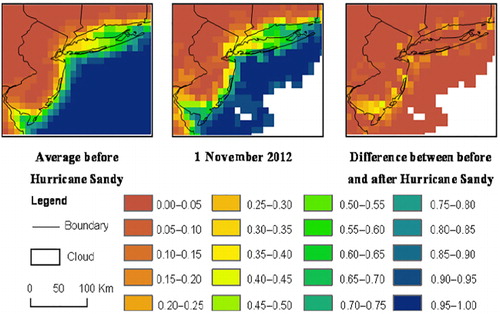
However, the spatial resolution from passive microwave sensor is usually very coarse (e.g. 15 km for the ATMS). The primary limitation of ATMS data for flood detection is its coarse spatial resolution (15 km²). It is difficult to obtain detailed information about the flood distribution from the original water fraction results because of the coarse resolution. According to the characters of water distribution in a basin, combining with high-resolution DEM data, high-resolution flood mapping can be obtained using the inundation model recently developed by Li et al. (2013a). By applying this inundation model and the DEM derived from the 30-m SRTM observations, water fraction and flood map derived from the ATMS can be enhanced to fine 30-m resolution. Figure 6 shows the flood map at 30-m resolution derived from the SRTM DEM data with the inundation model.

4.3. Evaluations

4.3.1. Comparison of a similar flood map produced by FEMA

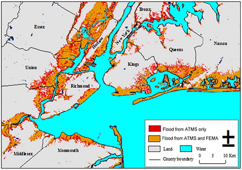
Compared with the flooding map derived from the VIIRS as shown in Figure 4, the ATMS 30-m flood map on 1 November 2012 shows consistent inundated locations with the flood zone maps from FEMA (Figure 4, lower). We further make a quantitative comparison of the SSF products distributed by FEMA (http://fema.maps.arcgis.com/home/index.html) during the Hurricane Sandy period. The SSF product, i.e. the flood information distributed by FEMA during Hurricane Sandy, included the states of NJ (New Jersey), NY (New York), and CT (Connecticut; Figure 6). For quantitative evaluation, the SSF product was re-sampled from 3-m to the same 30-m resolution and overlapped with our ATMS-derived flood map. The flood map derived from the ATMS and DEM data shows even more inundated area than the FEMA SSF product. Further quantitative assessment indicates a good agreement between the ATMS-derived and the FEMA SSF flood map (Figure 6) with a correlation of 0.95. One of the main sources for the remaining inconsistency or errors may be due to spatial resolution differences of the various datasets. Although we re-sampled all the datasets to the same 30-m spatial resolution, slight displacements of ATMS would cause a substantial shift in our ATMS-derived product, as it is compared with the fine 3-m resolution of the SSF product. Differences in the scope between ATMS-derived flood map and the SSF products can also be reasonably expected, because inland water inundation caused by hurricane-associated precipitation was not connected with the coastline or ocean. This type of flooding was reflected by microwave ATMS signal but was not included in the SSF products; thus, differences were observed when the two datasets were compared.

Figure 6. Thirty-meter resolution flood map generated from the ATMS and DEM on 1 November 2012, overlapped and compared with the FEMA SSF flood product.

4.3.2. Comparison of flood reports in crowd-contributed social media (Flickr)

In a next step, we compared our map to crowdsourced data from social media. The emergence of social media has provided another avenue for event reporting, with citizens contributing real-time information about breaking news. The popularity of platforms such as Twitter and Flickr and the substantial amount of content that is communicated through them are making social media a powerful open-source addition to authoritative datasets (Stefanidis, Crooks, and Radzikowski 2013). The information communicated through such feeds is often geolocated, and the analysis of this geospatial content may lead to the identification of patterns that can be correlated to physical events.

For this particular application, we focused on Flickr imagery. We collected all geolocated Flickr imagery that was posted reporting flooding in our study area within one week of the hurricane, and we compared these data to our ATMS-derived flood map. Our objective in this task is to assess the suitability of geotagged Flickr contributions to support remote sensing operations. These complements our earlier studies where we have shown the suitability of Twitter content to delineate the impact area of an earthquake (Crooks et al. 2013) and Flickr imagery to delineate the extend of wildfires (Panteras et al. 2015) and to provide a better view of the value of social media content to assess the impact of natural disasters.

We collected Flickr data through Flickr’s publicly accessible application programming interface. The Flickr data are images uploaded to the social media website over a weeklong period starting on 30 October 2012 that explicitly mention the words ‘flood’ and ‘Sandy’ in their descriptions. A total of 1059 geolocated images were obtained. In Figure 7, we see the spatial coincidence between these two datasets. It is found that 95% of the Flickr flood reports were distributed within the ATMS-derived flood area. We proceeded with the Flickr data in this case, rather than Twitter, because Twitter traffic was saturated with references to flooding even from locations that were not affected by it. The Flickr imagery was reasonably assumed to represent locations inside or adjacent to the flood zone (see Figure 7).

Figure 7. Flickr images reporting flooding (yellow dots) overlaid on the ATMS-derived flood map in the vicinity of New York City and its boroughs.

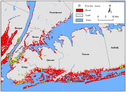
The significance of this finding is twofold. First, it offers a further argument for the quality of the ATMS-derived flood map. Second, and more importantly, this study presents a comparison of the spatial distribution of Flickr imagery that reports a flood event relative to the event itself at a large scale. The ground-level imagery that we used in this study was not contributed as a response to a specific request for data (as was the case in the work of Triglav-Cekada and Radovan (2013) during the Slovenian floods), but rather it was information contributed directly to Flickr by the general public as part of its normal social media activities. Therefore, it presents an unbiased representative example of social media content as it relates to flooding events. Accordingly, we argue that our results offer an early real data-based, large-scale study, which demonstrates the complementary nature of crowdsourced content (geotagged Flickr imagery, in this case) and remote sensing operations. This has been argued in the past but with very limited experimentation (see e.g. Poser and Dransch 2010; Schnebele and Cervone 2013; Roche et al. 2013).

5. Summary and discussions

The high temporal resolution and large coverage of coarse- to moderate-resolution satellite imagery, such as VIIRS and ATMS on board the NPP and future JPSS, are very advantageous for flood monitoring, but their coarse spatial resolution limits their wider application. Overcoming this limitation is an interesting scientific challenge with substantial application potential.

In this study, VIIRS observations are used to estimate floods induced by Hurricane Sandy along a coastline and New York area in late October and early November of 2012. But with the original resolutions, floods in small region cannot be identified, we therefore applied a recently developed inundation model to upscale VIIRS 375-m water fraction and flood maps to 30-m resolution by using the SRTM 30-m DEM data. It is found that flood map derived from VIIRS data shows less inundated area than the FEMA flood map and the ground observations. This is because optical sensor can only observe the Earth’s surface under clear-sky conditions, while clear data can only be found four days after the hurricane’s passing on 4 November 2012, when major floods due to Hurricane Sandy already receded. The peak floods were associated with cloudy conditions. Since microwave instruments, like radar and ATMS, can penetrate through clouds to watch the Earth’s surface, but the radar data are usually very expensive, we therefore developed a new method to derive flood maps from passive microwave ATMS observations. The flood map derived from the ATMS is also improved to 30-m spatial resolution by applying the same inundation model developed by Li et al. (2013c) and the SRTM 30-m DEM data.

To evaluate the flood mapping methodology presented in this study, we used corresponding datasets in the form of storm-tide site and HWM data and the FEMA 3-m-resolution Hurricane Sandy SSF products. Our assessment shows high consistency between our ATMS-derived 30-m flood maps and the validation data. Specifically, 88% of the storm-tide and HWM sites were located within the ATMS-mapped flood area. There was also a good agreement between ATMS- and FEMA-flooded areas, with an accuracy of 88% and a correlation of 0.94. Errors may be attributed to the soil moisture variations before and after the hurricane. Furthermore, when compared to ground-level geotagged contributions from social media, we found that 95% of the Flickr flood reports were similarly contained within our flood map. Overall, the proposed methodology was able to produce high-quality and high-resolution flood map over large-scale coastal areas.

Passive microwave observation is found useful and practical for SSF estimations, particularly for rainy and cloudy weather. Nevertheless, some key discussions that result from our study are as follows: (1) Because of the limited spatial resolution of the ATMS data, pure land or water pixels were very difficult to identify. Accordingly, prior knowledge of land samples and water samples based on land cover and river density can improve end-member accuracy. (2) Although we re-sampled the ATMS-derived flood map and FEMA SSF products to the same resolution for comparison, the spatial resolution differences of the various datasets may result in some inconsistencies or errors. (3) In our study, the ATMS data with small satellite zenith angles and daylight orbits were used for the flood estimation. A logical extension of this work would be to study the extent to which the satellite zenith angle and azimuth angle, solar zenith angle and azimuth angle affect the passive microwave signal. (4) Although passive microwave signal can penetrate through clouds, the resulting data, particularly from higher frequency channels, are still affected by precipitating clouds. Eliminating the effects of such clouds is another future research direction that emerges from this work. (5) The pixels’ soil moisture conditions may be different before and after flooding. The extent to which the soil moisture difference between pre- and post-flooding affects the water fraction difference may also need further investigations in the future. (6) Finally, we should also note that our approach is particularly geared toward large-scale floods, rather than small localized events.

Acknowledgments

The manuscript’s contents are solely the opinions of the authors and do not constitute a statement of policy, decision, or position on behalf of NOAA or NASA or the US Government. We appreciate the helpful and constructive comments from the reviewers.

Disclosure statement

No potential conflict of interest was reported by the authors.

Funding

The work was supported by the NOAA JPSS Program Office [grant number #NA12NES4400008] and by NASA Disaster Program [grant number #NNX12AQ74G].

References

- Bates, P. D., M. D. Wilson, M. S. Horritt, D. C. Mason, N. Holden, and A. Currie. 2006. “Reach Scale Floodplain Inundation Dynamics Observed Using Air Borne Synthetic Aperture Radar Imagery: Data Analysis and Modeling.” Journal of Hydrology 328 (1–2): 306–318. doi:10.1016/j.jhydrol.2005.12.028.
- Carroll, M. L., J. R. Townshend, C. M. DiMiceli, P. Noojipady, and R. A. Sohlberg. 2009. “A New Global Raster Water Mask at 250 m Resolution.” International Journal of Digital Earth 2 (4): 291–308. doi:10.1080/17538940902951401.
- Cho, K., and K. Nishiura. 2010. “A Study on Cloud Effect Reduction for Extracting Sea Ice Area from Passive Microwave Sensor Data.” Proceedings International Archives of the Photogrammetry, Remote Sensing and Spatial Information Science XXXVIII: 1042–1045.
- Choudhury, B. J. 1989. “Monitoring Global Land Surface Using Nimbus-7 37 GHz Data – Theory and Examples.” International Journal of Remote Sensing 10 (10): 1579–1605. doi:10.1080/01431168908903993.
- Crooks, A., A. Croitoru, A. Stefanidis, and J. Radzikowski. 2013. “#Earthquake: Twitter as a Distributed Sensor System.” Transactions in GIS 17 (1): 124–147. doi:10.1111/j.1467-9671.2012.01359.x.
- Ferraro, R. R., E. A. Smith, W. Berg, and G. J. Huffman. 1998. “A Screening Methodology for Passive Microwave Precipitation Retrieval Algorithms.” Journal of Atmospheric Science 55 (9): 1583–1600. doi:10.1175/1520-0469(1998)055<1583:ASMFPM>2.0.CO;2.
- Jin, Y. Q. 1999. “Flooding Index and Its Regional Threshold Value for Monitoring Floods in China from SSM/I Data.” International Journal of Remote Sensing 20 (5): 1025–1030. doi:10.1080/014311699213064.
- Li, S., D. L. Sun, M. D. Goldberg, and A. Stefanidis. 2013a. “Derivation of 30-m-resolution Water Maps from TERRA/MODIS and SRTM.” Remote Sensing of Environment 134: 417–430.
- Li, S., D. L. Sun, and Y. Yu. 2013b. “Automatic Cloud Shadow Removal from Flood/Standing Water Maps using MSG/SEVIRI Imagery.” International Journal Remote Sensing 34 (15): 5487–5502. doi:10.1080/01431161.2013.792969.
- Li, S., D. L. Sun, Y. Yu, I. Csiszar, A. Stefanidis, and M. D. Goldberg. 2013c. “A New Shortwave Infrared (SWIR) Method for Quantitative Water Fraction Derivation and Evaluation with EOS/MODIS and Landsat/TM data.” IEEE Transactions on Geoscience and Remote Sensing 51 (3): 1852–1862. doi:10.1109/TGRS.2012.2208466.
- Panteras, G., S. Wise, X. Lu, A. Croitoru, A. Crooks, and A. Stefanidis. 2015. “Triangulating Social Multimedia Content for Event Localization using Flickr and Twitter. Transactions in GIS. doi:10.1111/tgis.12122.
- Poser, K., and D. Dransch. 2010. “Volunteered Geographic Information for Disaster Management with Application to Rapid Flood Damage Estimation.” Geomatica 64 (1): 89–98.
- Roche, S., E. Propeck-Zimmermann, and B. Mericskay. 2013. “GeoWeb and Crisis Management: Issues and Perspectives of Volunteered Geographic Information.” GeoJournal 78 (1): 21–40. doi:10.1007/s10708-011-9423-9.
- Schnebele, E., and G. Cervone. 2013. “Improving Remote Sensing Flood Assessment Using Volunteered Geographical Data.” Natural Hazards and Earth System Science 13 (3): 669–677. doi:10.5194/nhess-13-669-2013.
- Sheng, Y., P. Gong, and Q. Xiao. 2001. “Quantitative Dynamic Flood Monitoring with NOAA AVHRR.” International Journal of Remote Sensing 22 (9): 1709–1724. doi:10.1080/01431160118481.
- Sippel, S. J., S. K. Hamilton, J. M. Melack, and B. J. Choudhury. 1994. “Determination of Inundation Area in the Amazon River Floodplain Using the SMMR 37 GHz Polarization Difference.” Remote Sensing of Environment 48 (1): 70–76. doi:10.1016/0034-4257(94)90115-5.
- Sippel, S. J., S. K. Hamilton, J. M. Melack, and E. M. M. Novo. 1998. “Passive Microwave Observations of Inundation Area and Area/stage Relation in the Amazon River Floodplain.” International Journal of Remote Sensing 19 (16): 3055–3074. doi:10.1080/014311698214181.
- Stefanidis, A., A. Crooks, and J. Radzikowski. 2013. “Harvesting Ambient Geospatial Information from Social Media Feeds.” Geojournal 78 (2): 319–338. doi:10.1007/s10708-011-9438-2.
- Sun, D. L., Y. Y. Yu, and M. D. Goldberg. 2011. “Deriving Water Fraction and Flood Maps from MODIS Images Using a Decision Tree Approach.” IEEE Journal of Selected Topics in Applied Earth Observations and Remote Sensing 4 (4): 814–825. doi:10.1109/JSTARS.2011.2125778.
- Sun, D. L., Y. Y. Yu, R. Zhang, S. Li, and M. D. Goldberg. 2012. “Towards Operational Automatic Flood Detection Using EOS/MODIS Data.” Photogrammetric Engineering and Remote Sensing 78 (6): 637–646. doi:10.14358/PERS.78.6.637.
- Tanaka, M., T. Sugimura, S. Tanaka, and N. Tamai. 2003. “Flood–Drought Cycle of Tonle Sap and Mekong Delta Area Observed by DMSP-SSM/I.” International Journal of Remote Sensing 24 (7): 1487–1504. doi:10.1080/01431160110070726.
- Triglav-Čekada, M., and D. Radovan. 2013. “Using Volunteered Geographical Information to Map the November 2012 Floods in Slovenia.” Natural Hazards and Earth System Science 13 (11): 2753–2762. doi:10.5194/nhess-13-2753-2013.
- Weng, F., H. Yang, and X. Zou. 2013. “On Convertibility from Antenna to Sensor Brightness Temperature for ATMS.” IEEE Geophysical Research Letters 10 (4): 771–775.
- Zheng, W., C. Liu, Z. X. Wang, and Z. B. Xin. 2008. “Flood and Waterlogging Monitoring over Huaihe River Basin by AMSR-E Data Analysis.” China Geographic Science 18 (3): 262–267. doi:10.1007/s11769-008-0262-7.