Numerical modeling and prediction of future response of permafrost to different climate change scenarios on the Qinghai–Tibet Plateau

Abstract

Projecting the future distribution of permafrost under different climate change scenarios is essential, especially for the Qinghai–Tibet Plateau (QTP). The altitude-response model is used to estimate future permafrost changes on the QTP for the four RCPs (RCP2.6, RCP4.5, RCP6.0, and RCP8.5). The simulation results show the following: (1) from now until 2070, the permafrost will experience different degrees of significant degradation under the four RCP scenarios. This will affect 25.68%, 40.54%, 45.95%, and 62.84% of the current permafrost area, respectively. (2) The permafrost changes occur at different rates during the periods 2030–2050 and 2050–2070 for the four different RCPs. (1) In RCP2.6, the permafrost area decreases a little during the period 2030–2050 but shows a small increase from 2050 to 2070. (2) In RCP4.5, the rate of permafrost loss during the period 2030–2050 (about 12.73%) is higher than between 2050 and 2070 (about 8.33%). (3) In RCP6.0, the permafrost loss rate for the period 2030–2050 (about 16.52%) is similar to that for 2050–2070 (about 16.67%). (4) In RCP8.5, there is a significant discrepancy in the rate of permafrost decrease for the periods 2030–2050 and 2050–2070: the rate is only about 3.70% for the first period but about 29.49% during the second.

Keywords:

• future permafrost changes
• Qinghai–Tibet Plateau
• altitude-response model
• temperature data
• VLRT
• RCPs

1. Introduction

Permafrost is one of the most important physical geographical phenomena that is sensitive to temperature, and climate change has a big effect on the distribution of alpine permafrost (Jiang et al. 2003). The Qinghai–Tibet Plateau (QTP) is underlain by the largest area of high-altitude permafrost in low-to-middle latitudes in the world and is especially susceptible to global climate change (Li et al. 2008). During the last several decades, the permafrost on the QTP has experienced widespread degradation because of the significant temperature increase that has occurred during this time (Zhao et al. 2004; Qin, Liu, and Li 2006; Wu and Zhang 2008; Wu, Zhang, and Liu 2011). Widespread permafrost degradation is likely to cause environmental deterioration, such as changes in surface hydrology and biochemical processes, increased desertification and destabilization of human infrastructure (Jin et al. 2000; Cheng and Wu 2007; Wang et al. 2000; Yang et al. 2010). Thus, understanding the future permafrost changes on the QTP has very important scientific significance. The purpose of this research is to simulate and analyze the spatial variation of permafrost at different periods under different models of the future climate so as to allow people to better cope with future environmental problems caused by changes in the permafrost.

Because the distribution of permafrost cannot be wholly obtained through field investigation, the mode method is considered an effective way of finding this out, especially for predictions of future changes in the permafrost. Although, there have been several studies into future permafrost changes on the QTP, there are some uncertainties in the models that were used. Also, the uncertainties in models of the future climate affect the accuracy of the permafrost simulations. For instance, Wang et al. (1996) forecast that the permafrost on the QTP would diminish dramatically by 2040 under a mean annual ground temperature (MAGT) increase of 0.4–0.5°C, mainly as a result of the disappearance of most of the present island of permafrost and the present shallow permafrost (thickness of less than 10 m). Jian (2000) used the averages for 1931–1960 and 2070–2099 from simulation results made by the general circulation model (GCM) as the Biome3 model input and concluded that the area of continuous permafrost on the QTP would mostly disappear and that the boundary of the discontinuous area would move northward by about 1–2°. Based on the GCM simulation results, Li and Cheng (1999) applied the ‘altitude model’ (in this study, we refer to this as the altitude-response model [ARM]) to predict the changes in permafrost on the plateau for 2009, 2049, and 2099. They found that the percentage of the total permafrost area that had disappeared would be no more than 19% in the subsequent 20–50 years, but that the decrease would be over 58% by the year 2099 for an average temperature increase on the QTP of 2.91°C. Using the MAGT model and taking an MAGT of 0.5°C as marking the boundary between permafrost and nonpermafrost, Nan, Li, and Liu (2002) considered that the amount of permafrost degradation over the subsequent 50 years would not be significant. In addition, Nan, Li, and Cheng (2005) predicted the permafrost changes on the plateau that would occur for heating rates of 0.02°C/year and 0.052°C/year. The results showed that, in response, in the first case, the permafrost area would decrease by 8.8% and 13.4% after 50 years and 100 years, respectively. The corresponding figures for the second case were 13.5% and 46.0%. Cheng and Liu (2008) used the high-resolution data produced by GCM under a mid-range emission scenario for greenhouse gases (A1B) as the input to two models, the MAGT model and the elevation model (in this study, we call this the ARM) to analyze the permafrost changes on the QTP for the periods 1980–1999, 2030–2049, and 2080–2099. It was found that the permafrost area would reduce by 31.82% and 45.89%, respectively, by 2030–2049 and 2080–2099. These studies provide a way to understand the future changes in the permafrost of the Tibetan Plateau that may occur. However, there are still great uncertainties in predicting the future state of the permafrost due to the low resolution of the future climate data that are used.

In this study, we collected and processed high-resolution temperature data produced by Fifth Assessment Report (AR5), temperature lapse rate data (VLRT), as well as latitude data and a digital elevation model (DEM). Based on these, the ARM was used to conduct a simulation and analysis of future changes in the permafrost for the years 2030, 2050, and 2070 under four RCP scenarios (RCP2.6, RCP4.5, RCP6, and RCP8.5) adopted by IPCC5.

2. Materials and methods

2.1. Study area

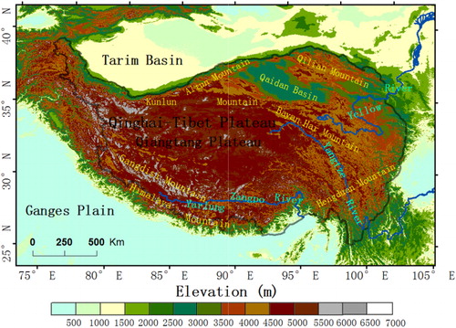
The Tibetan Plateau, stretching from 26.2° to 48.44° N and 73.0° to 104.4° E (an area of about 2.5 × 10⁶ km²) and having a mean elevation of more than 4000 m, is the largest and loftiest plateau in the world. Many high mountain ranges, including the Himalayas, Pamir, Kunlun Shan, and Qilian Shan, surround the plateau and constitute a unique geomorphic and climatic environment (Figure 1). This unique environment is the reason for the existence of a large area of permafrost (covering an area of 1.73 × 10⁶ km²) on the Tibetan Plateau. Meanwhile, the Tibetan Plateau is a storehouse of freshwater so bountiful that the region is the source of the headwaters of many of Asia’s largest rivers, including the Yellow, Yangtze, Mekong, Brahmaputra, Salween, and Sutlej, among others (Figure 1).

Figure 1. Topography and main rivers of the QTP.

2.2. Data sources

In our study, the data used consisted mainly of temperature, VLRT, and latitude data as well as a DEM. The sources of these data are described in the text that follows.

2.2.1. Temperature data

The future distribution of permafrost on the QTP was estimated by the ARM for several different emission scenarios. The temperature data included data for the present and future. Temperature is one of the most significant climatic factors that will determine future changes in the permafrost. The temperature data used were downloaded from the CCAFS climate data portal (http://www.ccafs-climate.org/). The ‘current’ data were used as the base data for estimating future changes in permafrost distribution. They were interpolated by the thin-plate smoothing spline algorithm, using latitude, longitude, and elevation as independent variables (Hijmans et al. 2005). The ‘future’ variables 2030 (the average temperature for 2021–2040), 2050 (the average for 2041–2060), and 2070 (the average for 2061–2080) were mainly obtained from the output of the GCM BCC-CSM1-1 for four RCP scenarios (RCP 2.6, RCP 4.5, RCP 6.0, and RCP 8.5). BCC-CSM1-1 was selected because it demonstrates the best performance for simulating temperatures in China (Xu and Xu 2012). The four RCPs were developed for climate change assessment and represent the radiative forcing levels for four greenhouse gas concentration (not emissions) trajectories. For RCP2.6, RCP4.5, and RCP6, global annual greenhouse gas emissions (measured as CO₂ equivalents) will respectively peak around the periods 2010–2020, 2040, and 2080, and then decline in each case. However, in RCP 8.5, emissions will continuously rise throughout the twenty-first century (Moss et al. 2008; Alexander et al. 2013). Meanwhile, the ‘future’ data were generated by downscaling and calibrating (bias correcting) the GCM output contained in the IPCC Fifth Assessment using WorldClim 1.4 as the baseline ‘current’ climate. All of these climate data – ‘current’ and ‘future’ – had a 30-second (latitude and longitude) spatial resolution, which is about 900 m at the equator. The ‘current’ temperature data together with the ‘future’ data for each time period are presented in Table 1.

Table 1. Temperature data (°C) for the QTP for four different IPCC5 RCPs.

		Temperature
RCPs	Period	Maximum	Minimum	Mean	Standard deviation
	current	24.24	−22.68	−1.39	5.09
RCP2.6	2030	25.50	−21.20	0.10	5.06
	2050	25.70	−20.90	0.21	5.08
	2070	25.60	−21.00	0.20	5.05
RCP4.5	2030	25.60	−21.00	0.20	5.07
	2050	26.00	−20.40	0.75	5.04
	2070	26.30	−20.10	1.07	5.02
RCP6.0	2030	25.40	−21.00	−0.04	5.03
	2050	26.00	−20.40	0.72	5.02
	2070	26.60	−19.70	1.41	5.01
RCP8.5	2030	26.60	−19.60	1.40	4.99
	2050	26.70	−19.60	1.51	5.03
	2070	27.7	−18.3	2.70	5.01

2.2.2. VLRT data

VLRT data is an important element in studying mountain climates (Rolland 2003). The average meteorological conditions of the upper air are relatively stable. Based on this, using the elevation and the air temperature of the 500, 600, and 700 hPa isobaric surfaces, Li and Xie (2006) produced an isocline map showing the annual average lapse rate using kriging interpolation. In order to acquire the VLRT, Li and Xie’s isocline map was scanned, geometrically corrected, projected, digitized, and interpolated. It was found that the lapse rate gradually varies from 0.699°C/100 m in the northwest of the QTP to 0.487°C/100 m in the southeast, which reflects the overall water vapor and thermal conditions.

2.2.3. DEM data

Shuttle Radar Topography Mission data with a spatial resolution of 3 arc-seconds (SRTM3) were downloaded for use as DEM data. This dataset includes a few missing values, which are filled using the mean values of the pixels in the surrounding 3 pixel × 3 pixel area. In addition, to ensure consistency, the SRTM3 data were resampled to 30-second spatial resolution.

2.2.4. Latitude data

Latitude is not only a significant factor that determines the distribution of permafrost on the QTP but also an important variable in the ARM (Cheng 1984). Therefore, we produced latitude data in grid format by assigning a latitude to each pixel, so that the latitude data had the same resolution as the other datasets.

2.3. Method

To simulate the geographical future distribution of permafrost on the QTP, four spatial modeling approaches have been put forward, including the altitude model (AM) (Cheng 1984), the MAGT model (Nan et al. 2002), the ‘Frost Number’ model (Nelson and Outcalt 1987), and the Temperature at the Top of Permafrost (TTOP) model (Smith and Riseborough 1996). The AM outputs the lower ‘boundary’ of the permafrost according to latitudinal position. The MAGT model estimates the MAGT and take the MAGT isotherm of 0.5°C as the boundary of permafrost and seasonal permafrost. The ‘Frost Number’ is manipulated by freezing and thawing degree-day ratios to define the permafrost continuity on an unambiguous latitudinal zonation. The TTOP describes the climate–permafrost relationship as a function linking the permafrost temperatures with the local surface and lithological conditions that control the ground thermal regime. This model is appropriate for small-scale estimations of permafrost temperatures. Nan et al. (2003) evaluated the suitability of these four models for the modeling of permafrost on the QTP and found that all four approaches were able to produce reasonable assessments of permafrost distribution. Based on the AM, the ARM approach was developed to estimate future changes in the distribution of permafrost on the QTP by including air temperature and VLRT data. The ARM is also much simpler and more practicable. Hence, many subsequent studies have used this model, especially for the prediction of permafrost distribution over long time periods (Jin et al. 2000; Wu, Zhang, and Liu 2001; Li et al. 2003; Cheng and Liu 2008; Cheng et al. 2012).

In this study, the ARM model was used for predicting the distribution of permafrost on the QTP under future climatic conditions. The permafrost distribution on the QTP has a distinct three-dimensional zonation, due to height, latitude, and aridity (or longitude). Based on these, the Gaussian distribution curve describing the correlation between the lower height limit of high-altitude permafrost (H) and latitude (φ) was calculated by Cheng (1984) as:

Using the AM, the lower limit for permafrost for each grid cell was calculated. By comparing this with the DEM (SRTM3 data) of the same resolution, it could then be determined whether or not the pixel contained permafrost. The following expression was used:

where P is a Boolean variable. P = 1 shows the existence of permafrost; P = 0 means permafrost is not present; and h is the altitude of the grid cell obtained from the DEM (SRTM3 data).

However, because the AM is a static model, it cannot describe the dynamic changes in permafrost distribution that occur in response to climate change. In order to overcome this problem, Li and Cheng (1999) introduced the variable ‘VLRT’ – the rate of decrease of atmospheric temperature with increasing elevation. The relationship between VLRT and elevation is expressed as:

where ΔH represents the change in elevation of the permafrost boundary, ΔT is the temperature change, and λ is the VLRT.

Over an area as large as the QTP, because the temperature is the most fundamental factor affecting the permafrost distribution, neglecting other elements, such as snow, precipitation, and solar radiation, is feasible (Cheng 1984). Meanwhile, Cheng (1984) also made three basic underlying assumptions. The first is that the function describing the ARM is stable under climate change. The second is that the spatial distribution of the VLRT on the QTP is also stable, which means that the vertical zonation will shift by a certain height for a specific temperature change, and the lower limit of the high-altitude permafrost will change by the same height. Third, lakes and glaciers can be neglected because of the huge differences between the total areas of glaciers and lakes and the permafrost. These are, respectively, about 4.66 × 10⁴ km² (Li et al. 1986) and 2.42 × 10⁴ km² (Yang, Li, and Yin 1983) for the glaciers and lakes and in excess of 1.20 × 10⁶ km² for the total area of the permafrost (Li and Cheng 1999).

3. Results and discussion

3.1. Simulation results and analysis

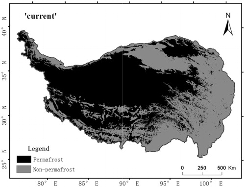
The future temperature data obtained from the CCAFS climate data portal (http://www.ccafs-climate.org/) were downscaled to a 1-km spatial resolution from the original output produced by GCMs by using the Delta statistical downscaling method based on the WorldClim dataset (1950–2000) as the baseline. Consequently, we used the ‘current’ temperature from the WorldClim dataset to describe the thermal conditions of the current period. In other words, we chose 1950–2000 average data as basic comparison data in the ARM. According to the ARM, the future distribution of permafrost can be simulated using temperature data, the VLRT, latitude, and a DEM (SRTM3). The simulated future areas of permafrost on the QTP for four RCPs were obtained (Table 2). Figure 2 and Table 2 show that, for each of the four RCPs, the permafrost is continuously degraded. From the present until 2030, the loss of permafrost area for the four RCPs (RCP2.6, RCP4.5, RCP6.0, and RCP8.5) is, respectively, 3.6 × 10⁵ km², 3.8 × 10⁵ km², 3.3 × 10⁵ km^2, and 6.7 × 10⁵ km², which account for 24.32%, 25.68%, 22.30%, and 45.27% of the area of the current permafrost (Tables 2 and 3). For the entire time span (from 1950–2000 to 2070), the corresponding losses in permafrost area are about 3.8 × 10⁵ km², 6.0 × 10⁵ km², 6.8 × 10⁵ km^2, and 9.3×10⁵ km², which account for 25.68%, 40.54%, 45.95%, and 62.84% of the current permafrost area, respectively (Tables 2 and 3). Considering just the permafrost changes from 2030 to 2050 and from 2050 to 2070, the following significant rules for the four RCPs were found. (1) In RCP2.6, there is essentially no degradation of the permafrost, and the permafrost area actually increases a little from 2050 to 2070. (2) In RCP4.5, the rate of permafrost loss from 2030 to 2050 (about 12.73%) is higher than from 2050 to 2070 (about 8.33%). (3) In RCP6.0, the permafrost loss rate for 2030–2050 (about 16.52%) is similar to that for 2050–2070 (about 16.67%). (4) However, in RCP8.5, the highest rate of permafrost decrease (about 29.49%) occurs between 2050 and 2070 and is about 25.79% higher than the loss rate for 2030–2050 (about 3.70%). Statistically, the degree and rate of permafrost loss in RCP8.5 are the highest and the total loss may reach 62.84% by 2070.

Table 2. Total areas of permafrost on the QTP for each period for the four RCPs (×10⁶ km²).

RCPs	current	2030	2050	2070
RCP2.6	1.48	1.12	1.09	1.10
RCP4.5		1.10	0.96	0.88
RCP6.0		1.15	0.96	0.80
RCP8.5		0.81	0.78	0.55

Table 3. The rate of permafrost degradation on the QTP during each period for the four RCPs (%). ‘+’ indicates permafrost degradation; ‘–’ indicates permafrost increase.

RCPs	From current to 2030	From 2030 to 2050	From 2050 to 2070	From current to 2070
RCP2.6	+24.32	+2.68	−0.92	+25.68
RCP4.5	+25.68	+12.73	+8.33	+40.54
RCP6.0	+22.30	+16.52	+16.67	+45.95
RCP8.5	+45.27	+3.70	+29.49	+62.84

Figure 2. Simulated ‘current’ permafrost distribution on the QTP.

According to the simulation results, the spatial variations of permafrost and nonpermafrost for the four RCPs on the QTP were analyzed first for each successive pair of periods (out of the present to 2030, 2030–2050, and 2050–2070) and then for the whole period – from the present to 2070. The changes in permafrost are divided into four categories: ‘increased permafrost,’ ‘decreased permafrost,’ ‘unchanged permafrost,’ and ‘unchanged nonpermafrost’ in Figure 3. The category ‘increased permafrost’ indicates seasonally frozen ground or persistently nonpermafrost conditions that have changed to permafrost. The category ‘decreased permafrost’ represents permafrost that has degraded to nonpermafrost. As a result of climate change, permafrost areas may become areas of nonpermafrost and, of course, the opposite may also occur. So, the categories ‘unchanged permafrost’ and ‘unchanged nonpermafrost’ describe whether the original permafrost regions or nonpermafrost regions have changed. In other words, ‘unchanged permafrost’ and ‘unchanged nonpermafrost’ mean that permafrost or nonpermafrost conditions have persisted over a particular time period. In the ARM, changes in the permafrost are mainly determined by the temperature. Overall, temperature values rise in the four RCPs. However, sometimes there are local decreases, which explain why there are some small increases in the number of permafrost pixels. Although these areas vary from period to period, they are mainly distributed in the southeast and southwest and along the boundary between the permafrost and nonpermafrost regions in the central parts of the QTP. For all four RCPs, the area of ‘increased permafrost’ is very small for all periods except for RCP8.5 from 2030 to 2050 – this increase occurs mainly in the southwest and along the boundary between the permafrost and nonpermafrost regions in the central parts of the QTP. Under all four scenarios, the area of ‘decreased permafrost’ is very obvious, particularly from the present until 2030 and between the present and 2070. These areas are mainly located at the boundary between the permafrost and nonpermafrost regions (Figure 3). The changes in area of the four permafrost categories for each period under the four RCPs scenarios are shown in Table 4. The spatial distribution of the four permafrost categories indicates that the ‘decreased permafrost’ is consistently the largest category from the present to 2030 and from the present to 2070 – the actual areas are different depending on the time period for the different RCPs. For the other two categories, the distributions have a high degree of consistency across the four RCPs. The area of ‘unchanged permafrost’ is mainly located in the western mountains, the Qiangtang Plateau and the Qilian Mountains, whereas the area of ‘unchanged nonpermafrost’ is mainly distributed along the boundary of the western mountains, the eastern and southeastern regions of the QTP and the Qaidam Basin.

Table 4. The areas (×10³ km²) of future permafrost changes for the four RCPs on the QTP.

RCPs	Period	Increased permafrost	Decreased permafrost	Unchanged permafrost	Unchanged nonpermafrost
RCP2.6	current–2030	0.1	363.1	1120.6	1169.9
	2030–2050	0.2	26.7	1094	1532.5
	2050–2070	3.2	6.8	1091	1552.7
	current–2070	0.1	386.2	1097.5	1169.9
RCP4.5	current–2030	0.1	386.6	1097.1	1169.9
	2030–2050	0	163.1	934.4	1556.2
	2050–2070	0	89.8	867.3	1696.6
	current–2070	0	603.9	879.8	1170.0
RCP6.0	current–2030	0.1	330.9	1152.8	1169.9
	2030–2050	0	190.5	962.8	1500.4
	2050–2070	0	161.7	801.6	1690.4
	current–2070	0	682	801.7	1170.0
RCP8.5	current–2030	0	669.8	813.9	1170.0
	2030–2050	21.5	54.5	759.8	1817.9
	2050–2070	0	227.5	554.1	1872.1
	current–2070	0	929.5	554.2	1170.0

Figure 3. Spatial distribution of future permafrost changes (from now to 2030, from 2030 to 2050, from 2050 to 2070, from 2030 to 2050, and from now to 2070) on the QTP for four RCPs. ‘Increased permafrost’ indicates seasonally frozen ground or persistently nonpermafrost conditions that have changed to permafrost. ‘Decreased permafrost’ represents permafrost that has degraded to nonpermafrost. ‘Unchanged permafrost’ and ‘Unchanged nonpermafrost’ means persistent permafrost and nonpermafrost conditions, respectively.

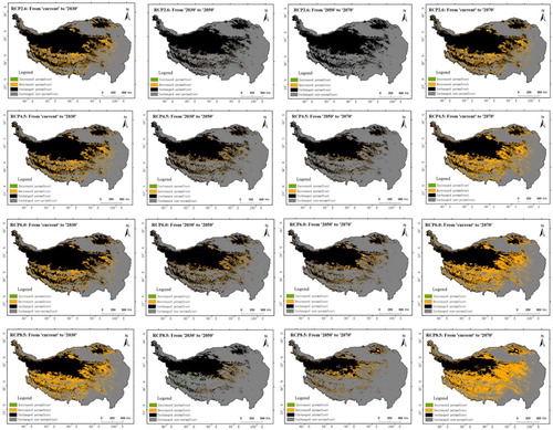
On the whole, under the four RCP scenarios (RCP2.6, RCP4.5, RCP6, and RCP8.5), the permafrost on the QTP will experience substantial degradation between now and 2070, and the area of permafrost will decrease; the maximum amount of degradation corresponds to RCP8.5 (Tables 2 and 3). The decrease in permafrost area mainly occurs around the southern and eastern borders of the southern and eastern Qiangtang Plateau, the southwestern mountains and the Qilian Mountains (Figure 3).

3.2. Accuracy assessment for the ARM

Using what is known about the distribution of permafrost on the QTP for recent decades, a series of empirical permafrost maps of China have been published, such as the 1:4,000,000 Snow, Ice and Permafrost Map of China (Shi and Mi 1988) and the 1:3,000,000 Permafrost Map of the QTP (Li and Cheng 1996), which were based on field survey data for different periods and on cartographical generalization. Moreover, several spatial permafrost models were created for assessing the geographical distribution of permafrost on the QTP, the parameters of which were based on measurements made at meteorological stations or remote sensing data. In order to assess the accuracy of the ARM, we compared the simulation results with these various permafrost data, which are listed in Table 5. The differences between the simulation results and the permafrost data summarized in Table 5 are small, except for the differences with the 1:3,000,000 Permafrost Map of the QTP and the MAGT model, for which the deviations are −24.32% and −16.89%, respectively (Wang et al. 2000). Differences in the map age, boundaries, and the scale used may be factors that lead to these inconsistencies. The 1:3,000,000 Permafrost Map was completed in 1996 (Li and Cheng 1996) and so essentially represented the distribution of permafrost in the 1990s (Zhao et al. 2012). By contrast, the AM was established on the basis of field data acquired in the 1970s. Also, there is a great difference between the outline of the QTP used in this study and that of 1:3,000,000 Permafrost Map of the QTP. Besides, all input data and simulations have a 30-second spatial resolution, which is about 900 m at the equator. This is a higher resolution than that of the 1:3,000,000 map of permafrost distribution on the QTP. Once these factors are taken into account, the simulation results produced by the ARM are generally credible.

Table 5. Total area of QTP underlain by permafrost according to published sources and different permafrost modeling approaches. Reference data used are the results of the simulation by the ARM (1.48 × 10⁶ km²), which represents the permafrost distribution under the current (1950–2000) climate conditions. ‘+’ indicates an increase; ‘–’ indicates a decrease.

Data source	Permafrost area(×10^6 km^2)	Deviation from reference data (%)	Note
Zhou and Guo (1982)	1.50	+1.35	Permafrost Map of China (compiled in 1975)
Xu and Wang (1983)	1.49	+0.68	1:4 M Map of Permafrost in China (compiled in 1978)
Shi and Mi (1988)	1.50	+1.35	1:4 M Map of the snow, Ice and Frozen Ground in China (1988)
Wang (1997)	1.23	−16.89	1:3 M Map of Permafrost Distribution on the QTP (Li and Cheng, 1996)
Nan (2003)	1.12	−24.32	MAGT model
Nan (2003)	1.28	−13.51	Surface frost number
Nan (2003)	1.39	−6.08	TTOP model

3.3. Advantages of the model

There are four main approaches (AM, MAGT, Frost Number model, and TTOP) to the spatial modeling of permafrost on the QTP and all four approaches are capable of providing a reasonable simulation of the distribution of permafrost on the QTP. However, Wu, Li, and Li (2000) showed that the AM has a higher accuracy than the MAGT model. In order to simulate the permafrost distribution on the QTP for different periods, the ARM was based on the AM. The ARM has been widely used to simulate the permafrost distribution on the QTP for different periods because of its accuracy and simplicity. Using this model, Li and Cheng (1999) predicted the permafrost distribution on the QTP in 2009, 2049, and 2099. Jin et al. (2000) forecast the response of permafrost on the QTP to climate change, and Cheng et al. (2012) used it to simulate the decadal permafrost distribution on the QTP over the past 50 years.

The data used as inputs to the ARM (temperature, VLRT and latitude data, and the DEM) are of high precision and quality. According to this model, the changes in the permafrost are mainly determined by the temperature, the future values of which are obtained from AR5.

The two temperature datasets obtained from IPCC AR5 and IPCC AR4 both performed well, and spatial correlation coefficients between the simulated and observed values of temperature were up to 0.96 (Xu and Xu 2012). AR5 could better capture the spatial distribution of the linear trend in surface temperature than AR4 for the period 1961–1999 in the QTP region (Guo et al. 2013). Using WorldClim 1.4 as the baseline ‘current’ climate (average temperatures for 1950–2000), the future temperature data were downscaled and calibrated (bias corrected) to a 30-second spatial resolution (about 900 m at the equator). This gave a high degree of consistency between the ‘current’ and ‘future’ temperature data, which can improve the accuracy of the ARM.

3.4. Limitations of the ARM

Although using the ARM has a number of advantages, inevitably, there are also some disadvantages. It is assumed that the function on which this model is based does not change in response to climate changes – this may cause a small discrepancy in the simulation results for other future periods (2030, 2050, and 2070). Additionally, ARM is a scenario-type model and cannot take into account the lag in permafrost changes.

Normally, the VLRT is a necessary parameter for studying mountain climate (Rolland 2003). In this study, the VLRT is obtained by kriging interpolation, which may be unsuitable in precise research. Moreover, the VLRT on the QTP may also vary a lot with time and location, which limits our confidence in the model to some extent. There will inevitably be some variability in the VLRT due to local environmental conditions, such as air mass type and local topography (Flenley 2007; Barry 2008). It is, therefore, very important to make further studies of the lapse rate on the QTP.

4. Conclusion

The permafrost conditions for 2030, 2050, and 2070 under the four RCPs–RCP2.6, RCP4.5, RCP6, and RCP8.5 – adopted by the IPCC5 – were simulated using the ARM. Through comparison with the results of previous studies (Table 5), the simulation results were seen to be reasonable and can, therefore, provide a basis for understanding the changes in the permafrost changes that might occur under different future climate scenarios.

Based on the simulation results, the other conclusions are as follows:

(1) For the entire time span considered (from now to 2070), the degraded permafrost areas for the four RCPs (RCP2.6, RCP4.5, RCP6.0, and RCP8.5) were 3.8 × 10⁵ km², 6.0 × 10⁵ km², 6.8 × 10⁵ km², and 9.3 × 10⁵ km², respectively, accounting for 25.68%, 40.54%, 45.95%, and 62.84% of the current permafrost area. This will cause serious environmental deterioration, including changes in surface hydrology, increased desertification, effects on biochemical processes, and destabilization of human infrastructure. Moreover, due to rapid permafrost degradation, large carbon pools sequestered in the permafrost could be released into the atmosphere again, resulting in a positive feedback effect and contributing to global warming.

(2) Considering only the permafrost changes from 2030 to 2050 and from 2050 to 2070, we found the following significant results. (1) In RCP2.6, permafrost degradation is not inevitable and even shows a small increase from 2050 to 2070. (2) In RCP4.5, the rate of permafrost loss from 2030 to 2050 (about 12.73%) is higher than from 2050 to 2070 (about 8.33%). (3) In RCP6.0, the permafrost loss rate for 2030–2050 (about 16.52%) is similar to that for 2050–2070 (about 16.67%). (4) In RCP8.5, the highest rate of permafrost loss (about 29.49%) occurs during the period 2050–2070 and is about 25.79% higher than the loss rate for the period 2030–2050 (about 3.70%).

(3) Persistent permafrost is mainly found in the western mountains, the Qiangtang Plateau and the Qilian Mountains. However, the permafrost loss occurs mainly around the southern and eastern borders of the southern and eastern Qiangtang Plateau, the southwestern mountains and the Qilian Mountains.

However, the ARM is a scenario-type model and cannot take into account lag times during permafrost degradation and formation. In order to characterize the response mechanism of alpine permafrost to climate change, a simulation model that can consider time lags and ground ice conditions should be constructed.

Acknowledgements

The temperature data used in this study were obtained from the CCAFS climate data portal (http://www.ccafs-climate.org/). We would like to thank the editors and the anonymous reviewers for very helpful suggestions that improved the article.

Disclosure statement

No potential conflict of interest was reported by the author.

Additional information

Funding

This research was funded by the Basic Research Project of the Ministry of Science and Technology of China [no. 2013FY110900] and the Science and Technology Plan Project of Yunnan Province [no. 2012CA021].

References

- Alexander, L., S. Allen, N. Bindoff, F. M. Breon, J. Church, U. Cubasch, S. Emori et al. 2013. Working Group I Contribution to the IPCC Fifth Assessment Report Climate Change 2013: The Physical Science Basis Summary for Policymakers, 2–36.
- Barry, R. G. 2008. Mountain Weather and Climate. Boulder, CO: Cambridge University Press.
- Cheng, G. D. 1984. “Problems on Zonation of High-altitudinal Permafrost.” Acta Geographica Sinica 39 (2): 185–193. ( in Chinese)
- Cheng, G. D., and T. H. Wu. 2007. “Responses of permafrost to climate change and their environmental significance, Qinghai-Tibet Plateau.” Journal of Geophysical. Research Earth Surface 112 (F2): F02S03
- Cheng, Z. G., and X. D. Liu. 2008. “A Preliminary Study of Future Permafrost Distribution on the Qinghai-Tibet Plateau under Global Warming Conditions.” Areal Research and Development 27: 80–85. ( in Chinese)
- Cheng, W. M., S. M. Zhao, C. H. Zhou, and X. Chen. 2012. “Simulation of the Decadal Permafrost Distribution on the Qinghai-Tibet Plateau (China) over the Past 50 Years.” Permafrost and Periglacial Processes 23 (4): 292–300. doi:10.1002/ppp.1758.
- Flenley, J. R. 2007. “Ultraviolet Insolation and the Tropical Rainforest: Altitudinal Variations, Quaternary and Recent Change, Extinctions, and Biodiversity.” In Tropical Rainforest Responses to Climatic Change, edited by M. B. Buch and J. R. Flenley, 219–235. Chichester: Praxis.
- Guo, Y., W. J. Dong, F. M. Ren, Z. C. Zhao, and J. B. Huang. 2013. “Surface Air Temperature Simulations over China with CMIP5 and CMIP3.” Advances in Climate Change Research 4 (3): 145–152. doi:10.3724/SP.J.1248.2013.145.
- Hijmans, R. J., S. E. Cameron, J. L. Parra, P. G. Jones, and A. Jarvis. 2005. “Very High Resolution Interpolated Climate Surfaces for Global Land Areas.” International Journal of Climatology 25 (15): 1965–1978. doi:10.1002/joc.1276.
- Jin, H. J., S. X. Li, G. D. Cheng, S. L. Wang, and X. Li. 2000. “Permafrost and Climatic Change in China.” Global and Planetary Change 26 (4): 387–404. doi:10.1016/S0921-8181(00)00051-5.
- Jian, N. 2000. “A Simulation of Biomes on the Tibetan Plateau and their Responses to Global Climate Change.” Mountain Research and Development 20 (1): 80–89. doi:10.1659/0276-4741(2000)020[0080:ASOBOT]2.0.CO;2.
- Jiang, F. C., X. H. Wu, S. B. Wang, Z. Z. Zhao, and J. L. Fu. 2003. “Basic Features of Spatial Distribution of the Limits of Permafrost in China.” Journal of Geomechanics 9 (4): 303–312. ( in Chinese)
- Li, S. D., and G. D. Cheng. 1996. Map of permafrost distribution on the Qinghai–Xizang (Tibetan) Plateau (1:3 000 000). Lanzhou: Gansu Cultural Press. ( in Chinese)
- Li, X., and G. D. Cheng. 1999. “A GIS-aided Response Model of High Altitude Permafrost to Global Change.” Science in China, Ser. D 42 (1): 72–79. doi:10.1007/BF02878500.
- Li, X., G. D. Cheng, H. J. Jin, E. Kang, T. Che, R. Jin, L. Z. Wu, Z. T. Nan, J. Wang, and Y. P. Shen. 2008. “Cryospheric Change in China.” Global and Planetary Change 62 (3–4): 210–218. doi:10.1016/j.gloplacha.2008.02.001.
- Li, X., G. D. Cheng, Q. B. Wu, and Y. J. Ding. 2003. “Modeling Chinese Cryospheric Change by Using GIS Technology.” Cold Regions Science and Technology 36 (1–3): 1–9. doi:10.1016/S0165-232X(02)00075-7.
- Li, Q. Y., and Z. C. Xie. 2006. “Analyses on the Characteristics of the Vertical Lapse Rates of Temperature.” Journal of Shihezi University (Natural Science) 24 (6): 719–723. ( in Chinese)
- Li, J. J., B. X. Zheng, X. J. Yang, Y. Q. Xie, L. Y. Zhang, Z. H. Ma, and S. Y. Xu. 1986. Glaciers of Xizang (Tibet). Beijing: Science Press (in Chinese).
- Moss, R., M. Babiker, S. Brinkman, E. Calvo, T. Carter, J. Edmonds, I. Elgizouli et al. 2008. Towards New Scenarios for Analysis of Emissions, Climate Change, Impacts, and Response Strategies. Geneva: Intergovernmental Panel on Climate Change, 132.
- Nan, Z. T. 2003. “Study of the Characteristics of Permafrost Distribution on the Qinghai-Tibet Plateau and Construction of Digital Roadbed of the Qinghai-Tibet Railway.” Ph.D Dissertation of Cold and Arid Regions Environmental and Engineering Research Institute, Chinese Academy of Sciences. ( in Chinese)
- Nan, Z. T., S. X. Li, and G. D. Cheng. 2005. “Prediction of Permafrost Distribution on the Qinghai-Tibet Plateau in the Next 50 and 100 years.” Science in China Ser. D 48 (6): 797–804. doi:10.1360/03yd0258.
- Nan, Z. T., S. X. Li, and Y. Z. Liu. 2002. “Mean Annual Ground Temperature Distribution on the Tibet Plateau: Permafrost Distribution Mapping and Further Applications.” Journal of Glaciology and Geocyology 24 (2): 142–148. ( in Chinese)
- Nelson, F.E., and S. I. Outcalt. 1987. “A Computational Method for Prediction and Regionalization of Permafrost.” Arctic and Alpine Research 19 (3): 279–288. doi:10.2307/1551363.
- Qin, D. H., S. Y. Liu, and P. J. Li. 2006. “Snow Cover Distribution, Variability, and Response to Climate Change in Western China.” Journal of Climate 19 (9): 1820–1833. doi:10.1175/JCLI3694.1.
- Rolland, C. 2003. “Spatial and Seasonal Variations of Air Temperature Lapse Rates in Alpine Regions.” Journal of Climate 16 (7): 1032–1046. doi:10.1175/1520-0442(2003)016<1032:SASVOA>2.0.CO;2.
- Shi, Y. F., and D. S. Mi. 1988. Map of Snow, Ice and Frozen Ground in China (1: 4 000000). Beijing: Cartographic. ( in Chinese)
- Smith, M.W., and D. W. Riseborough. 1996. “Permafrost Monitoring and Detection of Climate Change.” Permafrost and Periglacial Processes 7 (4): 301–309. doi:10.1002/(SICI)1099-1530(199610)7:4<301::AID-PPP231>3.0.CO;2-R.
- Wang, S. L. 1997. “Study of Permafrost Degradation in the Qinghai-Xizang Plateau.” Advanced in earth sciences 12 (2): 164–167.
- Wang, S. L., H. J. Jin, S. X. Li, and L. Zhao 2000. “Permafrost Degradation on the Qinghai-Tibet Plateau and its Environmental Impacts.” Permafrost and Periglacial Process 11 (1): 43–53. doi:10.1002/(SICI)1099-1530(200001/03)11:1<43::AID-PPP332>3.0.CO;2-H.
- Wang, S. L., X. F. Zhao, D. X. Guo, and Y. Z. Huang. 1996. “Response of Permafrost to Climate Change in the Qinghai-Xizang Plateau.” Journal of Glaciology and Geocyology 18: 157–165. ( in Chinese)
- Wu, Q. B., X. Li, and W. J. Li. 2001. “The Response Model of Permafrost along the Qinghai–Tibetan Highway under Climate Change.” Journal of Glaciology and Geocryology 23 (1): 1–6. ( in Chinese)
- Wu, Q. B., X. Li, and W. J. Li. 2000. “Computer Simulation and Mapping of the Regional Distributionof Permafrost along the Qinghai-Xizang Highway.” Journal of Glaciology and Geocryology 22 (4): 323–326. ( in Chinese)
- Wu, Q. B., and T. J. Zhang. 2008. “Recent Permafrost Warming on the Qinghai-Tibetan Plateau.” Journal of Geophysical Research 113: D13108. doi:10.1029/2007JD009539.
- Wu, Q. B., T. J. Zhang, and Y. Z. Liu. 2011. “Thermal State of the Active Layer and Permafrost along the Qinghai-Xizang (Tibet) Railway from 2006 to 2010.” The Cryosphere 5 (5): 2465–2481. doi:10.5194/tcd-5-2465-2011.
- Xu, X. Z., and J. C. Wang. 1983. “Preliminary Discussion on the Distribution of Frozen Ground and its Zonality in China.” In Proceedings of 2nd National Conference on Permafrost (Selection), edited by Lanzhou Institute of Glaciology and Cryopedology, Chinese Academy of Sciences, 3–12. Lanzhou: Gansu People’s.
- Xu, Y., and C. Xu. 2012. “Preliminary Assessment of Simulations of Climate Changes over China by CMIP5 Multi-models.” Atmospheric and Oceanic Science Letters 5 (6): 489–494.
- Yang, Y. C., B. Y. Li, and Z. S. Yin. 1983. Geomorphology of Xizang (Tibet). Beijing: Science Press.
- Yang, M. X., F. E. Nelson, N. I. Shiklomanov, D. L. Guo, and G. N. Wan. 2010. “Permafrost Degradation and its Environmental Effects on the Tibetan Plateau: A Review of Recent Research.” Earth-Science Reviews 103 (1–2): 31–44.
- Zhao, S. M., W. M. Cheng, C. H. Zhou, X. Chen, and J. Chen. 2012. “Simulation of Decadal Alpine Permafrost Distributions in the Qilian Mountains over Past 50 Years by Using Logistic Regression Model.” Cold Regions Science and Technology 73: 32–40. doi:10.1016/j.coldregions.2011.12.006.
- Zhou, Y. W., and D. X. Guo. 1982. “Major Features of Permafrost in China.” Journal of Glaciology and Geocryology 4 (1): 1–19. ( in Chinese)
- Zhao, L., C.-L. Ping, D. Q. Yang, G. D. Cheng, Y. J. Ding, and S. Y. Liu. 2004. “Changes of Climate and Seasonally Frozen Ground over the Past 30 Years in Qinghai–Xizang (Tibetan) Plateau, China.” Global Planetary Change 43 (1–2): 19–31. doi:10.1016/j.gloplacha.2004.02.003.