Monitoring land surface and cover in urban and peri-urban environments using digital aerial photography

Abstract

This paper describes the development of a system for decimetre-scale monitoring of land-surface and land-cover in urban and peri-urban environments. We describe our methodology that comprises the application of highly automated processing and analysis methods to digital aerial photography. The approach described in this paper addresses a monitoring need by providing the ability to generate change information at a spatial resolution suitable for urban, peri-urban and coastal areas, where an increasing percentage of the worlds’ population dwells. These areas are dynamic, with many environmental issues associated with planning, service provision, resource management and allocation, as well as monitoring regulatory compliance. We present a system based on standardised data and methods, which is able to track and communicate changes in features of interest in a way that has not been previously possible. We describe the methodology and then demonstrate its feasibility by applying it to geographic areas of planning and policy relevant size (the order of tens of thousands of square kilometres). We demonstrate the approach by applying it to the problem of urban forest assessment.

Keywords:

• monitoring
• urban forest
• aerial remote sensing

1. Introduction

Growing populations and urbanisation increases the intensity of the use of both natural and built resources and thus the scale of future impacts from planning choices on cities and surrounding areas. Key considerations for planners and policy makers include the impact of urbanisation on the natural environment and environmental services such as air and water quality management, economic viability, urban heat islands and population density. Typically these will be managed by a multitude of agencies working for different entities, including national, state and local government departments, private and public enterprises and community groups. Understanding the social-ecosystem interactions and their governance may be improved by taking an integrative view of the processes involved at an appropriate scale (Borgström et al. 2006). The process of planning, communicating and monitoring the implementation of various programs can be aided by quantitative assessments of their efficacy (Pauleit and Duhme 2000). Such assessments, in a general urban and peri-urban setting, may be at an individual, local authority or city scale. Better coordination of planning and action in this multifaceted environment will benefit a number of areas including, for example, wetland (Davis and Froend 1999) and vegetation management (Wallace et al. 2008).

Using the reporting on nature reserves as an example, information relevant to such questions as ‘What is the state of this reserve at present relative to its past, and how does this compare with other reserves?’ and ‘How are different areas in the reserve responding to endogenous and exogenous stresses?’ may be derived from time-series remotely sensed data. Such questions are often part of regional assessments used for informing planning and policy decisions (e.g. Planning 2012; Strategic Assessment 2012).

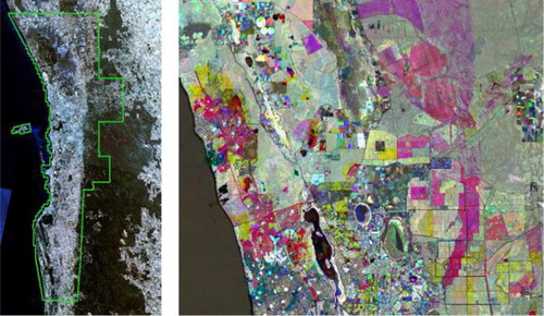
The potential for the use of remotely sensed optical satellite data (at varying resolutions) in urban environments has long been considered; see for example the reviews provided by Jensen and Cowen (1999) and Herold, Scepan, and Clarke (2002). A relatively large imaging footprint from a sensor with stable acquisition parameters lends itself to forming consistent data over large geographic areas from which time-varying attributes may be observed. A simple example of a ‘photosynthetically active’ vegetation index, or more specifically the Normalised Difference Vegetation Index (NDVI) (Tucker 1979) derived from calibrated time-series Landsat TM data for the northern Perth region is provided in Figure 1. In this depiction, shades of grey indicate regions that have not changed, hot colours represent reduction in vegetative cover (caused largely by the impact of fire and clearing of vegetation for new housing developments) and cool colours represent gains (largely recovery in natural systems and the establishment of gardens in new urban developments). This simple example highlights the ability of the sensor to detect change in a consistent manner over large areas and also the dynamic nature of urban and peri-urban regions.

Figure 1. (Left) The extent of the study area is depicted by the green boundary overlaid on the satellite image of the greater Perth region. (Right) Urban areas are dynamic, as demonstrated by this three-date NDVI composite with the NDVI from 1990, 1998 and 2008 displayed in red, green and blue, respectively. Areas having shades of grey are stable in this display, hot colours represent vegetation decline and cool colours represent vegetation gain.

Though multispectral optical satellite data are useful for many purposes, the modern spatial resolutions of half a metre in panchromatic and metres in multispectral are greater than the 10–30 cm ground sample distance (GSD) typically acquired from aerial platforms by local and state government for planning purposes. For this reason we concentrate our efforts on examining the potential of digital aerial photography, although we note the advancements in other areas including sensors and their combined use (see for example the reviews by Gamba 2014; Gamba, DellAcqua, and Dasarathy 2005; Zhang 2010) and the possibilities for incorporating more systems in the future (see, for example, Brook, Ben-Dor, and Richter 2013).

Aerial photography is an important source of spatial data, which historically has required a great deal of manual interpretation to elicit useful information (Fensham and Fairfax 2002). The digitisation of photography has allowed increasing automation to be applied in the processing workflows. Digital aerial photography offers the possibility of providing new information, including reflectance estimates and other derived information, in a highly automated manner. Acquired at regular time steps, it can form the basis of a monitoring system (Honkavaara et al. 2009). With radiometrically calibrated data, spatial-temporal information similar to that depicted in Figure 1 may be achieved. Simple indices derived from the calibrated data may also be used in comparative city analysis, such as the visible impervious surface analysis proposed many years ago by Ridd (1995). Deriving consistent information from digital aerial photography is complicated by the multitude of land and resource uses, the complex natural and built nature of the environment, and the variable viewing and solar geometry across the tens of thousands of images typically required for large cities.

The complexity is evident in past and present research, which have considered algorithms that attempt to specifically identify subsets of urban elements, for example cars (Grabner et al. 2008), buildings and trees (Haala and Brenner 1999; Meng et al. 2012) and impervious surfaces (Hodgson et al. 2003). More recent attempts have aimed to provide complete semantic descriptions of all elements in an image (Kluckner et al. 2010). For complex urban scenes a combination of spectral and morphological information is typically required to discriminate classes such as trees from grassed areas or streets from buildings (Haala and Brenner 1999). These areas have similar spectral properties but varying morphological properties. In this paper we also adopt methods based on spectral and morphological properties.

In this paper we describe our methodology and demonstrate its application to the task of estimating the distribution and extent of vegetation height over a city sized area. In Section 2 we describe the data collected, and the method used to generate radiometrically calibrated orthographically projected photographs (orthophotos) and digital elevation data. There is much current active research in the radiometric calibration of aerial optical data to ground reflectance (e.g. Haest et al. 2009; Alverez et al. 2010; Lopez et al. 2011; Collings et al. 2011) representing various combinations of empirical and physical modelling. Some of the complications in achieving good radiometric calibration are caused by incomplete descriptions of various measurement systems (Honkavaara et al. 2009; Markelin et al. 2010; Cramer 2009). We exploit recent empirical methods for image calibration described by Collings et al. (2011), which offer some flexibility by statistically modelling some of the effects.

Apart from being a requirement for deriving trend information, geometrically and radiometrically consistent data aids in automation of the derivation of class label information such as maps of green space, roads and trees. Automation is important because of the volume of data and the fine scale of information required for policy making. In Section 3 we provide examples of deriving thematic products through the analysis of calibrated data in conjunction with ground observations and other spatial data. In Section 4 we comment on the successes and limitations of the described approach.

2. Material and methods

2.1. Data

Wide-scale data collection over the greater Perth area (approximately 9600 square kilometres) commenced on 14 March 2007, where approximately 35,000 frames of data over a period of 19 cloud free days were acquired. The instrument was a Microsoft UltraCAM-D digital frame camera (Leberl and Gruber 2003) flown at a height of about 1300 m. Each frame consists of red, green, blue and near-infrared band radiance along with a panchromatic image. The nominal acquisition was for 65% forward and 30% side overlap. The GSD was approximately 30 cm and 10cm for the multispectral and panchromatic data, respectively. These parameters resulted in approximately 12 terabytes of primary data. The on-board hardware allowed for approximately 4 hrs of continuous acquisition with these parameters. The season corresponds to the dry, hot Mediterranean summer experienced by the city at this time of year. In order to minimise the effect of solar angle (and in particular, shadowing) on the images, flying was constrained to 2 hrs each side of solar noon. The field of view of each frame was approximately 50°. The data were preprocessed to Level 2 (Leberl and Gruber 2003), using Vexcel UltraCAM proprietary software, which is designed to account for instrument-specific effects but not atmospheric or bidirectional reflectance distribution function (BRDF) effects. The dynamic range of the data as captured by the camera was preserved (i.e. the data were not converted to 8 bit quantisation or compressed using routines converting the data to JPEG formats).

Acquisitions were repeated in 2008 and 2009, though with some adjustment to the acquisition specifications towards angular as opposed to time: latter acquisitions specified the window of capture via sun angle specifications. For 2008 and 2009, two 3-hr windows either side of solar noon, were used to achieve 6 hrs of acquisition per day. In this paper we concentrate on results obtained at the time of writing, which were derived from the 2007 and 2009 data.

We note that for 2010, 2011, 2012, 2013, 2014 and 2015 data for the region were acquired as part of the State Land Information Capture Program (SLICP) using the more recently available Leica ADS40 and ADS80 systems. The more recent acquisitions tended to take fewer days than those we examine here, reflecting the evolution of hardware (e.g. better on-board storage, different systems etc). The new data are similar to that of the early acquisitions in that red, green, blue and near-infrared were captured and the dynamic range preserved, but the instruments differ in parameters such as their band pass characteristics and geometric configurations (frame vs push-broom for instance). Switching to SLICP acquisition meant that the data were collected as part of the state government’s annual program of capture of the area. This reduces the cost to users, standardises products and encourages applications to be developed with the knowledge that there will be on-going routine data acquisition.

2.2. Geometric registration and surface models

All frames went through a rigorous photogrammetric process including aerial triangulation, generation of Digital Surface Models (DSM) and orthorectification using the derived DSM. The aerial triangulation was jointly performed by Landgate (Western Australia) and the CSIRO. Initially, the on-board inertial measurement unit data were used for image orientation. About one hundred tie points per image and many ground control points were collected semimanually using INPHO software. PATB software was used to conduct the aerial triangulation (with self-calibration mode).

The DSM was generated using in-house software based on the method described by Wu (1995, 1996). The method used grid-based relaxation matching algorithms applied to epipolar images. Reliable matching points were then gridded to form the final DSM. High-performance computing was a necessity for processing the data. Parallel OpenMP implementations of the algorithms were executed on cluster computing resources located at iVEC, Western Australia’s supercomputing centre.

Figure 2 graphically depicts typical results of the DSM generation and the orthorectification. The accuracy of the DSM was assessed against the state’s triangulated tie points and an independent set of ground control check points.

Figure 2. Primary monitoring data consist of radiometrically calibrated true orthophotos. Digital surface models are generated for each time epoch. Shown are examples of the DSM for 2007 and 2009 (left and middle) and a local example of the orthophoto and corresponding DSM (bottom and top right, respectively).

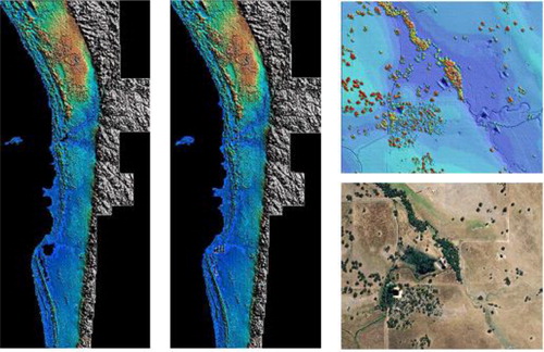
Table 1 contains the results of the elevation differences between the DSM and the triangulated tie points, and between the DSM and the check points. From the table we observe that RMS errors of less than half a metre in elevation were achieved.

Table 1. The accuracy assessment of elevation differences between the DSM and triangulated tie points, and the DSM and independent check points.

	Triangulation tie points		Independent check points
Block names	Points	RMS (m)	Points	RMS (m)
Gnangara	383,489	0.182	453	0.457
Perth	518,802	0.246	16,348	0.393
Woorooloo	50,291	0.238	320	0.440
Wungong	10,786	0.264	26	0.334
South	327,858	0.198	1794	0.428
Rottnest	2402	0.319	37	0.346

RMS, root mean squared error.

The majority of the independent check points have recorded measurements of either hatch cover height or ground level height. We note that none of the independent check points were checked physically in the field against the DSM and orthophotos. So for example, if by chance a measurement was associated with a road that had since been resurfaced, then these heights may be invalid.

In order to more closely validate the DSM elevation accuracy, 36 independent check points covering an open area of approximately 12 km by 8 km were measured by a Landgate surveyor using a differential GPS unit (accuracy better than 5 cm). The RMS of the elevation differences between the DSM and these 36 points was 0.165 m, which is much smaller than the results obtained using unchecked points. For well-matched (high scores obtained from cross-correlation matching) open areas, an RMS error less than 0.2 m for the DSM may therefore be assumed. Of course, there were many small localised areas where the absolute error of the DSM was larger. Reasons include image quality, weather conditions and limitations of automated matching, especially in the dense urban areas (buildings, trees) and along the roads (due to vehicle movement).

For use in further analysis, we generate from the DSM a Digital Terrain Model (DTM) and a normalised DSM (nDSM) for each date. The DTM is simply an estimate of the ground elevation, and the nDSM is an estimate of the height of all elements relative to the ground. For the sake of brevity, we refer the reader to, for example Kraus and Pfeifer (1998), on the concept of nDSM from DSM.

Here the DTM was generated by firstly identifying a set of candidate ground points from the DSM using segmentation followed by filtering of outliers; and secondly creating a spatially contiguous surface by fitting a set of thin plate splines to the candidate ground points. Curvature is the key parameter in the outlier detection algorithm, with points having a curvature greater than a user-specified threshold rejected from inclusion in the candidate ground set. Different parameter settings were used to control the filtering of outliers in the forested hills in the east compared with flat urbanised coastal plain in the west. In the forested hills, a higher curvature threshold was used to avoid hilltops and valley bottoms being falsely rejected. A lower curvature threshold was specified for the coastal plain to reject built structures not identified by the morphological filter. The mostly open-canopy native forests and urbanised areas yielded sufficiently dense ground candidate points for interpolation. This was due in part to correlation matching being applied to every image pixel used to generate the DSM. Candidate ground points were sparser in pine plantations, and largely comprised roads and logging tracks. See Hingee (2013) for details.

2.3. Radiometric calibration to ground reflectance

To automatically track changes in a time-series of images requires that the same land-cover viewed at different times has the same spectral signature. This can be achieved by radiometrically calibrating the time-series to a reference image (called the radiometric base [Furby and Campbell 2001]) or to some other standard. We have chosen ground reflectance as our standard.

For vicarious calibration of the imagery to known reference values, painted fibreboard targets were deployed throughout the region at the time of acquisition. The targets were measured in the laboratory with an ASD FieldSpec Pro spectrometer, which was calibrated with a Spectralon reference plate, both before and after deployment. The stiff, flat targets were painted in matte white, grey or black to ensure the greatest consistency in reflection with minimum deviation from Lambertian behaviour. The size of the targets, 120 cm × 120 cm, was chosen so that at least one image pixel, expressed as GSD, would lie entirely within a given target, while at the same time considering the operational practicalities of deploying targets using standard utility vehicles. Larger targets could be constructed by forming arrays of these basic targets, but have not been considered to date with the preference being to get targets deployed over a larger geographic extent. Targets were deployed at multiple geographically dispersed sites in the acquisition region. Deployment was on flat open ground in sets of three, consisting of black, grey and white targets co-located in an area of interest, thus providing low-,medium- and high-reflectance ground truths for calibration purposes.

Reflectances for the white, grey and black targets were fairly consistent for the visible and near infrared region of interest for each target, with values around 0.85, 0.35 and 0.05, respectively. In subsequent years (2010 onward), two additional intermediate shades of grey were included to add more reflectance points for fitting and/or validation.

The calibration was achieved by employing statistical models that include BRDF kernels to reduce inconsistencies due to differing viewing and illumination angles, and gain and offset parameters to compensate for variations in atmospheric and camera settings. The BRDF and atmospheric/instrument effects were modelled using the Li sparse BRDF kernel (Roujean, Leroy, and Deshchamps 1992), K, with multiplicative and additive constants. Treating each band independently, the digital number d_ik of the k^th pixel in image i was modelled as:

(1)

where:d_ik = the digital number of the k^th pixel of image i

R_ik = the relative reflectance of the k^th pixel of image i

ξ = a vector consisting of the solar zenith angle, view zenith angle and relative azimuth angle.

K = Li sparse BRDF kernel

K_i = the mean of K over the i^th image

β_i1 = kernel weight

β_i2 = the “constant kernel” weight for the i^th image j ^th band

α_i = the multiplicative term for image.

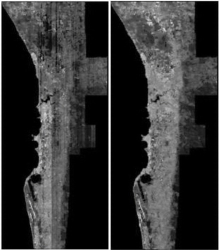
The model (1) was fitted to the image data by minimising the cost function, which incorporated an overlap penalty term and spatial smoothness constraints. The overlap penalty term improves consistency between neighbouring images. The spatial smoothness constraints avoid over-fitting of image-based kernel parameters while allowing for the parameters to vary by image frame for differing cover types. The details are described by Collings and Caccetta (2013), with indicative results (for the year 2007) replicated in Figure 3.

Figure 3. Radiometric calibration of the aerial imagery. (a) Before calibration and (b) after calibration. Reflectance estimates were within 4.4, 9.9 and 18.7% of absolute reflectance as recorded for the black, grey and white painted targets, respectively (Collings and Caccetta 2013).

For the results presented in Section 3, we ignored variations in reflectance estimates due to terrain illumination variations (such as bright and dark sides of roofs, trees) and areas in shadow. For the former, our method of classification, which is based on rational polynomials, partially compensates for this effect. For the latter, there are known methods based on ray tracing to estimate the position of the shadow using a digital surface model (Wu, Collings, and Caccetta 2010) or physical modelling of the spectra (Makarau et al. 2011) that may be applied in future work. For the results presented here, we have not applied such shadow detection methods.

Once the data were geometrically and radiometrically aligned, they were prepared as 1:25,000 map sheets closely corresponding to the standard cadastral map series for the region. This facilitates the data management and subsequent use by other agencies using standard software and hardware.

2.4. Land cover analysis and estimating vegetation distribution

Given the nDSM and the radiometrically corrected true orthophoto for each year, classifications were derived for each year using simple rules. Since we did not correct explicitly for terrain illumination effects in the spectral information, the derivation of spectral indices and subsequent classifications were based on ratios of variables.

In the first instance, classification was performed using only spectral data (near-infrared, red, blue and green bands). The heights, from the nDSM, were then used to discriminate between cover types that were not spectrally separable, such as some types of trees and bushes (above-ground) and grass (on-ground).

Generally for multiclass land cover classifications, we base our classifications on decision boundaries applied to discriminant functions derived using canonical variate analysis (CVA) with rational polynomials (CVAR) (Chia, Campbell, and Caccetta 2004; Hingee 2013). In standard CVA the data x is transformed linearly into y = c₁ ^tx. CVAR differs by transforming the data into y = (c₁ ^tx)/(a + c₂ ^tx), where ‘a’ is a constant (we chose a = 1 usually) and the vectors c₁ and c₂ are chosen to maximise the ratio of the between-groups and within-groups variance of the transformed data. We note here that the NDVI is a member of this class of functions, often used for vegetation studies. CVAR provides an approach for deriving similar normalised indices that can be tailored to discriminate other land cover classes of interest.

In the example to follow, we restrict our attention to the two-class discrimination problem of forming an estimate of the spatial distribution of green space, which is of specific interest to our research partners. For this restricted class set, thresholding of the NDVI performed adequately and required less spatial stratification compared with indices we derived from analysis of ground data using CVAR.

Given the large data volumes (10’s of terabytes) resulting from having a data resolution of the order of 20 cm, the methods and workflows were based on using the greatest possible degree of automation, combined with some manual intervention to improve the final accuracy of the results. A Quality Assurance process was embedded within the workflow to ensure that standards were met and record the level and form of intervention taken. The workflow therefore contained automated methods, manual quality checks, manual interventions, recording of the interventions and the level of interventions taken and documentation of known remaining limitations.

Given the radiometrically corrected orthophotos and the nDSM, the following steps were applied to each 1:25,000 map tile:

1. Classify green space versus non-green space using a threshold applied to the NDVI, then remove roofs having high NDVI values using a morphological rule. This identifies all green growing vegetation, including for example grass, bushes and trees.

2. Label each pixel in the green space classification according to the nDSM values to produce a ‘VegHeight’ image. This variable may be stratified into categories such as grass, which is at ground height, or trees that are 2.0 m or more (2.0 m is used as the height criteria in Australia’s forest definition).

3. Perform and record the results of a quality check of the results. This process may return to previous steps if required. Three different levels of checking are recorded as: (1) no manual inspection; (2) manual inspection and errors documented, but not fixed and (3) manual inspection and some errors remedied using manual digitisation.

4. Compare results to estimate accuracy statistics.

5. Calculate vegetation summary statistics.

3. Results and discussion

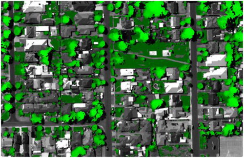
The methodology was applied to data from the years 2007 and 2009 and where vegetation was present its height was recorded as raster images (an example of which is depicted in Figure 4). Two dates were processed as a test of how well the methodology could be replicated from year to year. Figure 4 shows an example of the vegetation height map, with details of grassed areas, including parks and lawn, street trees as well as smaller shrubs and bushes easy to distinguish.

Figure 4. Depiction of the vegetation height for the year 2007 overlaid on a grey scale aerial photograph. In this figure, the height of the vegetation is indicted by its brightness in green, ordered from dark to bright green representing low to high vegetation height, respectively.

The vegetation classification was compared with the validation data and the site counts recorded in Tables 2–5. Along with the site counts, summary statistics of the overall, producer and users accuracy are provided. Classes considered were vegetation, non-vegetation, tree and non-tree labelled as veg, non-veg, tree and non-tree in the tables respectively. From Tables 2 and 3 we observe overall accuracies of the order of 90%, though the method underestimates (compared to manual interpretation) the vegetation by up to 27% at site 2. This site in particular had a lot of unirrigated grasslands, as well as non-green standing vegetation, which was not captured by the classifier. This poses an interpretation problem; if such vegetation is to be included, these sites may warrant further stratification, strata-specific thresholds and perhaps more tailored indices and subsequent classifier based on CVAR.

Table 2. Vegetation accuracy for the year 2007.

		Manual interpretation
Class label		Non-veg	Veg	Total	Users (%)
Site 1	Non-veg	158	8	166	95
	Veg	6	88	94	94
	Total	164	96	260
	Producers (%)	96	92		Overall = 95
Site 2	Non-veg	740	49	789	94
	Veg	7	132	139	95
	Total	747	181	928
	Producers (%)	99	73		Overall = 94
Site 3	Non-veg	167	4	171	98
	Veg	4	56	60	93
	Total	171	60	231
	Producers (%)	98	93		Overall = 97

The overall accuracy of the classifier compared with manual interpretation was above 94% for the three sites.

Table 3. Vegetation accuracy for the year 2009.

		Manual interpretation
Class label		Non-veg	Veg	Total	Users (%)
Site 1	Non-veg	165	16	181	91
	Veg	0	79	79	100
	Total	165	95	260
	Producers (%)	100	83		Overall = 94
Site 2	Non-veg	673	60	733	92
	Veg	33	162	195	83
	Total	706	222	928
	Producers (%)	95	73		Overall = 90
Site 3	Non-veg	172	3	175	98
	Veg	2	54	56	96
	Total	174	57	231
	Producers (%)	99	95		Overall = 98

The overall accuracy of the classifier compared with manual interpretation was above 90% for the three sites.

From Tables 4 and 5 we observe overall accuracies equal to or better than 90%, though with an underestimate (compared to manual interpretation) of tree canopy ranging from 25% (site 3, 2009) of up to 48% (site 2, 2009). For this class, the omission of tree canopy was largely due to (1) general underestimation of the extent of individual tree crowns (particularly the edges of the canopy) and (2) the 2m height definition with the omitted canopy classed as vegetation in the non-tree class.

Table 4. Tree accuracy for the year 2007.

		Manual interpretation
Class label		Non-tree	Tree	Total	Users (%)
Site 1	Non-tree	186	22	208	89
	Tree	4	48	52	92
	Total	190	70	260
	Producers (%)	98	69		Overall = 90
Site 2	Non-tree	781	68	849	92
	tree	1	78	79	99
	Total	782	146	928
	Producers (%)	100	53		Overall = 93
Site 3	Non-tree	207	7	214	97
	tree	4	13	17	78
	Total	211	20	231
	Producers (%)	98	64		Overall = 95

The overall accuracy of the classifier compared with manual interpretation was 90% or above for the three sites. The classifier underestimates the area of tree as compared with the human operator in each of the three sites.

Table 5. Tree accuracy for the year 2009.

		Manual interpretation
Class label		Non-tree	Tree	Total	Users (%)
Site 1	Non-tree	190	23	213	89
	Tree	0	47	47	100
	Total	190	70	260
	Producers (%)	100	67		Overall = 91
Site 2	Non-tree	760	80	840	90
	Tree	1	87	88	99
	Total	761	167	928
	Producers (%)	100	52		Overall = 91
Site 3	Non-tree	212	4	216	98
	Tree	3	12	15	80
	Total	215	16	231
	Producers (%)	99	75		Overall = 92

The overall accuracy of the classifier compared with manual interpretation greater than 90% for the three sites. The classifier underestimates the area of tree as compared with the human operator in each of the three sites.

Next, the average height of the vegetation and the variance of the height of vegetation were calculated and plotted in log form (so that the areas of lower height classes fit in the y axis) for all height classes in Figure 5 for each year. The results are summarised in Table 6. From Figure 5 we observe that the estimates obtained from 2007 to 2009 show no major departures across the height range. In Table 6 we firstly observe slightly differing overall captured area between the years, of the order of ~1% variation in area. This is due to different patterns of missing data between time-steps, including data gaps, occlusion by smoke and similar. We also note a reduction in the percentage of vegetation between 2007 and 2009 for all height classes, with the largest percentage reduction coming from the vegetation in the lowest height class. This class is most susceptible to the effect of shadowing and temporal variation due to irrigation (rainfed or otherwise). The vigour of grasses and hence their detectability from photography varies significantly with local weather and irrigation regimes over periods of a few days in the high temperatures experienced at the time of year of image acquisition.

Figure 5. Area of trees [log₁₀(Area_Trees_km²)] by height (m) for the years 2007 and 2009. The estimates show no major departure across the height range.

Table 6. Vegetation summary statistics for the region for the years 2007 and 2009.

	Vegetation summary
	2007 sq. km. (and % of area captured)	2009 sq. km. (and % of area captured)
Area captured	9396 (100)	9303 (100)
Area of vegetation	3219 (34.2)	2583 (27.7)
Area of vegetation above 10 m	413 (4.4)	400 (4.3)
Area of vegetation between 2 and 10 m	884 (9.4)	851 (9.1)
Area of vegetation between 0.5 and 2 m	464 (4.9)	394 (4.2)
Area of vegetation below 0.5 m	1494 (15.9)	937 (10.1)
Height distribution of vegetation of height 2 m or more
Mean height of vegetation above 2 m	8.23 m	8.25 m
Standard deviation of vegetation above 2 m	5.12 m	5.07 m

Next we turn our attention to trees, which are of direct interest to local government. The Tree area and height statistics are summarised by local government area for the year 2007 and 2009 in Tables 7 and 8, respectively. In the tables, the greyed entries identify those local government areas that were not fully covered by the aerial capture. For those local government areas that had full aerial coverage, the % area of trees is typically in the range 10–20%. The local government areas that are marked with an asterix (incomplete coverage) have higher percentages than the summaries provided below, as the region to the east that is not covered by aerial capture is mostly native forested areas. Estimates are relatively consistent from year to year, which one would expect within a two-year period, with a notable exception being that for the City of Wanneroo where the tree canopy area almost halved in this period. This result coincided with the relatively large-scale harvest of pine plantations in the nonurbanised north of the area. This latter example highlights the ability of the approach to detect and provide diagnostic evidence for changes occurring within local government management areas.

Table 7. Tree canopy and height summary by local government area for the years 2007.

	Year 2007 tree area and height
	Area km^2		Tree height
Locality	Estimate	%	Mean	Std	Total non-null area km^2
MANDURAH, CITY OF	27.69	14.28	6.71	8.01	193.88
WANNEROO, CITY OF	112.82	16.26	9.37	10.93	693.67
COCKBURN, CITY OF	16.68	9.66	5.98	7.09	172.69
JOONDALUP, CITY OF	10.50	10.16	6.22	7.48	103.34
EAST FREMANTLE, TOWN OF	0.42	11.77	6.21	7.06	3.57
FREMANTLE, CITY OF	1.81	9.32	6.35	7.43	19.38
CLAREMONT, TOWN OF	1.04	20.85	7.33	8.57	4.96
COTTESLOE, TOWN OF	0.55	14.05	6.11	7.09	3.91
CAMBRIDGE, TOWN OF	4.37	19.86	7.16	8.51	22.01
VINCENT, CITY OF	1.49	13.08	6.97	8.34	11.38
SUBIACO, CITY OF	1.47	21.13	7.99	9.30	6.97
PEPPERMINT GROVE, SHIRE OF	0.29	27.55	7.39	8.48	1.06
STIRLING, CITY OF	12.64	12.06	6.65	7.87	104.76
VICTORIA PARK, TOWN OF	2.27	12.75	7.97	9.52	17.82
BASSENDEAN, TOWN OF	1.63	15.79	7.04	8.27	10.31
MOSMAN PARK, TOWN OF	0.67	15.60	6.42	7.47	4.31
NEDLANDS, CITY OF	4.58	23.02	6.97	8.18	19.89
BAYSWATER, CITY OF	3.80	11.63	6.69	7.88	32.65
SOUTH PERTH, CITY OF	3.21	16.35	7.19	8.61	19.63
MELVILLE, CITY OF	7.41	14.07	6.61	7.88	52.66
CANNING, CITY OF	6.76	10.46	6.50	7.64	64.58
BELMONT, CITY OF	3.47	8.82	6.78	7.89	39.36
GOSNELLS, CITY OF	17.66	13.92	7.09	8.28	126.87
KWINANA, TOWN OF	15.92	13.32	6.62	8.00	119.48
ROCKINGHAM, CITY OF	28.71	11.30	7.41	9.08	254.12
PERTH, CITY OF	0.86	10.76	8.78	10.52	7.95
*SWAN, CITY OF	146.54	14.90	8.12	9.49	983.51
*KALAMUNDA, SHIRE OF	69.49	30.99	8.81	10.13	224.23
*MUNDARING, SHIRE OF	106.08	21.53	8.46	9.86	492.58
*ARMADALE, CITY OF	81.00	21.45	8.75	10.17	377.59
*SERPENTINE-JARRAHDALE, SHIRE OF	135.69	18.98	8.68	10.20	714.73
*WAROONA, SHIRE OF	79.36	14.86	9.09	10.73	534.10
*CHITTERING, SHIRE OF	80.35	9.97	7.04	8.06	805.60
*MURRAY, SHIRE OF	85.61	8.68	7.74	9.00	986.79
*HARVEY, SHIRE OF	105.18	16.68	9.62	11.19	630.43
*NORTHAM, SHIRE OF	3.44	9.74	7.22	8.25	35.28
*TOODYAY, SHIRE OF	7.45	13.09	6.82	7.95	56.91
*WANDERING, SHIRE OF	8.78	15.02	8.05	9.51	58.50
*GINGIN, SHIRE OF	98.51	8.48	7.41	8.89	1161.15

*Entries correspond to incomplete spatial coverage for the shire.

Table 8. Tree canopy and height summary by local government area for the year 2009.

	Year 2009 tree area and height
	Area km^2		Tree height
Locality	Estimate	%	Mean	Std	Total non-null area km^2
MANDURAH, CITY OF	25.41	12.83	6.80	8.04	198.06
WANNEROO, CITY OF	64.77	9.35	8.21	9.89	692.53
COCKBURN, CITY OF	18.25	10.65	6.15	7.28	171.42
JOONDALUP, CITY OF	10.91	10.65	6.26	7.54	102.44
EAST FREMANTLE, TOWN OF	0.50	14.07	6.19	7.04	3.56
FREMANTLE, CITY OF	1.90	9.81	6.32	7.38	19.33
CLAREMONT, TOWN OF	0.90	18.19	7.57	8.82	4.96
COTTESLOE, TOWN OF	0.54	13.72	6.14	7.14	3.92
CAMBRIDGE, TOWN OF	3.69	16.79	7.31	8.65	21.97
VINCENT, CITY OF	1.45	12.73	7.05	8.43	11.37
SUBIACO, CITY OF	1.33	19.09	8.10	9.39	6.96
PEPPERMINT GROVE, SHIRE OF	0.24	22.17	7.61	8.74	1.06
STIRLING, CITY OF	12.29	11.74	6.62	7.84	104.67
VICTORIA PARK, TOWN OF	2.23	12.49	7.59	9.06	17.83
BASSENDEAN, TOWN OF	1.47	14.23	7.21	8.44	10.32
MOSMAN PARK, TOWN OF	0.67	15.55	6.42	7.47	4.31
NEDLANDS, CITY OF	3.54	17.80	7.39	8.64	19.89
BAYSWATER, CITY OF	3.63	11.27	6.55	7.73	32.20
SOUTH PERTH, CITY OF	2.85	14.52	7.45	8.87	19.63
MELVILLE, CITY OF	7.22	13.70	6.74	8.02	52.66
CANNING, CITY OF	6.56	10.15	6.50	7.70	64.67
BELMONT, CITY OF	3.45	8.75	6.60	7.71	39.39
GOSNELLS, CITY OF	19.13	15.06	7.24	8.44	126.96
KWINANA, TOWN OF	17.07	14.28	6.99	8.45	119.53
ROCKINGHAM, CITY OF	27.68	10.79	7.64	9.26	256.42
PERTH, CITY OF	0.73	9.17	8.75	10.19	7.94
*SWAN, CITY OF	126.22	12.83	8.00	9.26	984.13
*KALAMUNDA, SHIRE OF	62.85	28.03	8.91	10.26	224.21
*MUNDARING, SHIRE OF	94.18	19.03	8.48	9.89	494.86
*ARMADALE, CITY OF	101.50	26.80	8.60	10.01	378.67
*SERPENTINE-JARRAHDALE, SHIRE OF	146.73	20.46	8.63	10.08	717.02
*WAROONA, SHIRE OF	89.99	16.83	9.33	10.87	534.57
*CHITTERING, SHIRE OF	72.66	8.99	7.27	8.23	808.55
*MURRAY, SHIRE OF	107.83	10.95	8.48	9.77	985.11
*HARVEY, SHIRE OF	103.25	16.25	9.95	11.47	635.26
*NORTHAM, SHIRE OF	4.64	13.06	7.84	8.83	35.50
*TOODYAY, SHIRE OF	7.64	13.26	6.96	7.86	57.60
*WANDERING, SHIRE OF	12.90	22.05	7.85	9.42	58.49
*GINGIN, SHIRE OF	81.43	7.00	7.10	8.60	1163.23

*Entries correspond to incomplete spatial coverage for the shire.

4. Conclusion

In this paper we have described the conceptual design and some key technical aspects of establishing a fine-scale monitoring system based on digital aerial photography. The spatial resolution of the system was chosen with the view toward providing information relevant for planning activities at local, district and city scale.

We described the generation of a geometric and radiometric base and our current work on land cover classification. Fensham and Fairfax (2002) described the considerable potential of aerial photography for assessing vegetation presence and its change, and also identified the standardisation of image contrast and geometric consistency as the major limitations to successful broad-scale application. This work demonstrates a solution to these limitations using modern digital instruments. The results were obtained by processing a large number of very high-resolution images per time-step, captured using a high-resolution digital camera, with the integration of the more recent push-broom Leica ADS40/80 data in progress. The results demonstrate the feasibility of extrapolating classifiers across large geographic areas of aerial photography, provided it is appropriately geometrically and radiometrically calibrated. The calibration allows the methodology to be replicated, providing consistent results for two independent acquisitions from 2007 to 2009. Consistent with others’ findings in the literature, we found that spectral discrimination was limited and that classification accuracies were significantly improved when the 3D aspect of the data was used.

The vegetated component of the study region was mostly open canopy, and sufficient estimates of ground elevation were able to be inferred from the photography. The incorporation of LiDAR observations would be beneficial where (1) denser canopy scenarios are encountered; (2) extra information on canopy structure is desired or (3) acquiring photography with minimal shadow is problematic. MacFaden et al. (2012) provide an excellent recent example of the application of LiDAR to mapping urban canopy and other elements having these properties. For the first time in this region, estimates of the spatial distribution of vegetation by height were produced at a GSD of 20 cm, and subsequently summarised by local government area, providing planning relevant information used in part in the Western Australian Government’s ‘City Planning Framework’ (Planning 2012). The information is being used for quantifying the extent and structure of the urban canopy; establishing goals and planting criteria; providing a means for monitoring outcomes and public communication. Particular examples include assessment of bird habitat and planning of tree planting programs to offset the loss of vegetation as a result of the intensification of urban land use.

Prior to this work, the standard approach to mapping vegetation in this region was manual digitisation of the boundaries of vegetated areas. Vegetation communities were represented as a boundary, attributed with coarse descriptors tagged to a point within the boundary. Manual digitisation was performed on aerial photography projected onto a coarse DTM, and subsequently onto a coarse DSM, typically generated from an earlier acquisition. Errors in the spatial accuracy of elevated feature boundaries were the result. These interpretations were often in plan-view, were not updated regularly and heights were not recorded.

Though we demonstrate the utility of the monitoring system applied to vegetation assessment, a time-series of surface heights and ground reflectance estimates is useful more generally, especially when integrated with other spatial data and sensors such as thermal and hyperspectral imaging, LiDAR and dense time-series from satellite sensors. For example, surface albedo and thermal measurements are important parameters for investigating urban heat island effects (Hart and Sailor 2009) and power usage in relation to roofing materials (Simpson and McPherson 1997); Akbari, Konopacki, and Pomerantz 1999; Shen, Tan, and Tzempelikos 2011). Estimates of the actual temperatures would be achieved by thermal measurements and/or imaging.

Aerial photography has been acquired over the urban area considered in this paper for decades on at least an annual basis. This is also the situation for many urban areas around the world. The data are routinely used by all levels of government for a multitude of purposes, and it is likely that the data will continue to be collected. The cost to monitor land surface and cover therefore becomes the incremental cost associated with processing it to a standard format and deriving a set of useful products from it. Though joint acquisition is increasingly common, other observations such as obtained from LiDAR, thermal and hyperspectral instruments are not acquired so regularly, and the RGBI cameras used with joint captures are typically to a lower specification of resolution and accuracy than that used for more traditional mapping. Therefore, we expect that time sequences of high-quality aerial photography will have an important role for long-term monitoring, enhanced with the observations of other sensors’ unique characteristics when and where required.

Acknowledgements

The authors would like to thank Landgate for their efforts for the aerial triangulation processing of aerial image data and for providing the check points for the DSM accuracy assessment. The authors would also like to thank iVEC for providing the computation and storage facilities for the storage and processing of the data. Financial contributions for data acquisition and processing were provided by the state and federal government. We would also like to thank our colleagues who deployed the radiometric ground targets each year.

Disclosure statement

No potential conflict of interest was reported by the authors.

References

- Akbari, H., S. Konopacki, and M. Pomerantz 1999. “Cooling Energy Savings Potential of Reflective Roofs for Residential and Commercial Buildings in the United States.” Energy 24 (5): 391–407. doi:10.1016/S0360-5442(98)00105-4.
- Alverez, F., T. Catanzarite, J. R. Rodriquez-Perez, and D. Nafria 2010. “Radiometric Calibration and Evaluation of UltraCam X and Xp Using Portable Reflectance Targets and Spectrometer Data. Application to Extract Thematic Data from the Imagery Gathered by the Nation Plan of Aerial Orthophotography. Proceedings of EuroCOW2010, 10.2–12.2, Castelldefels.
- Borgström, S. T., T. Elmqvist, P. Angelstam, and C. Alfsen-Norodom. 2006. “Scale Mismatches in Management of Urban Landscapes.” Ecology and Society 11 (2): 16.
- Brook, A., E. Ben-Dor, and R. Richter. 2013. “Modelling and monitoring urban built environment via multi-source integrated and fused remote sensing data.” International Journal of Image and Data Fusion 4 (1): 2–32. doi:10.1080/19479832.2011.618469.
- Collings, S. and, P. A. Caccetta. 2013. “Radiometric Calibration of Very Large Digital Aerial Frame Mosaics.” International Journal of Image and Data Fusion, 4 (3): 214–229. doi:10.1080/19479832.2012.760656.
- Collings, S., P. A. Caccetta, N. A. Campbell, and X. Wu. 2011. “Empirical Models for Radiometric Calibration of Digital Aerial Frame Mosaics.” IEEE Transactions on Geoscience and Remote Sensing 49 (7): 2573–2588. doi:10.1109/TGRS.2011.2108301
- Chia, J., N. A. Campbell, and P. A. Caccetta. 2004. “Using rational Polynomials for Mapping in Areas with Terrain without Using a Digital Elevation Model.” Proceedings 12th Australasian Remote Sensing and Photogrammetry Conference, Fremantle Western Australia, >October 18–22, on CD-ROM.
- Cramer, M. 2009. Digital Camera Calibration, European Spatial Data Research (EuroDSR). Official Publication No. 55, 257 p. ISBN: 978-9-051-79658-2.
- Davis, J. A., and R. Froend. 1999. “Loss and Degradation of Wetlands in Southwestern Australia: Underlying Causes, Consequences and Solutions.” Wetlands Ecology and Management 7: 13–23.
- Fensham, R. J., and R. J. Fairfax. 2002. “Aerial Photography for Assessing Vegetation Change: A Review of Applications and the Relevance of Findings for Australian Vegetation History.” Australian Journal of Botany 50: 415–429.
- Furby, S. L., and N. A. Campbell. 2001. “Calibrating Images from Different Dates to Like-value Counts.” Remote Sensing of Environment 77: 186−196.
- Gamba, P. 2014. “Image and Data Fusion in Remote Sensing of Urban Areas: Status Issues and Research Trends.” International Journal of Image and Data Fusion 5 (1): 2–12.
- Gamba, P., F. DellAcqua, and B.V. Dasarathy. 2005. “Urban Remote Sensing Using Multiple Data sets, Past, Present and Future.” Information Fusion 6: 319–326.
- Grabner, H., T. T. Nguyen, B. Gruber, and H. Bischof. 2008. “On-line Boosting-based Car Detection from Aerial Images.” ISPRS Journal of Photogrammetry and Remote Sensing 63 (3): 382–396. doi:10.1016/j.isprsjprs.2007.10.005.
- Haala, N., and C. Brenner. 1999. “Extraction of Buildings and Trees in Urban Environments.” ISPRS Journal of Photogrammetry and Remote Sensing 54 (2–3): 130–137. doi:10.1016/S0924-2716(99)00010-6.
- Haest, B., J. Biesemans, W. Horsten, J. Everaerts, N. Van Camp, and J. Valckenborgh. 2009. “Radiometric Calibration of Digital Photogrammetric Camera Image Data.” Proceedings of the ASPRS 2009 Annual Conference, Baltimore, MA, March.
- Hart, M. A., and D. J. Sailor. 2009. “Quantifying the Influence of Land-use and Surface Characteristics on Spatial Variability in the Urban Heat Island.” Theoretical and Applied Climatology 95 (3–4): 397–406.
- Herold, M., J. Scepan, and K. C. Clarke. 2002. “The Use of Remote Sensing and Landscape Metrics to Describe Structures and Changes in Urban Land Uses.” Environment and Planning A 34 (8):1443–1458.
- Hingee, K. H. 2013. “Ground Elevation Models and Land Cover Classiers for Decimetre Resolution Urban Monitoring.” Thesis submitted to Curtin University of Technology, Perth, Western Australia.
- Hodgson, M. E., J. R. Jensen, J. A. Tullis, K. D. Riordan, and C. M. Archer. 2003. “Synergistic Use of Lidar and Color Aerial Photography for Mapping Urban Parcel Imperviousness.” Photogrammetric Engineering & Remote Sensing 69 (9): 973–980. doi:10.14358/PERS.69.9.973.
- Honkavaara, E., R. Arbiol, L. Markelin, L. Martinez, M. Cramer, S. Bovet, L. Chandelier, R. et al. 2009. “Digital Airborne Photogrammetry—A New Tool for Quantitative Remote Sensing?—A State-of-the-Art Review On Radiometric Aspects of Digital Photogrammetric Images.” Remote Sensing 1: 577–605.
- Jensen, J. R., and D. C. Cowen. 1999. “Remote Sensing of Urban/Suburban Infrastructure and Socio-economic Attributes.” Photogrammetric Engineering and Remote Sensing 65 (5): 611–622.
- Kluckner, S., T. Mauthner, P. M. Roth, and H. Bischof. 2010. “Semantic Classification in Aerial Imagery by Integrating Appearance and Height Information.” Computer Vision – ACCV 2009, Lecture Notes in Computer Science, Vol. 5995, 477–488, Berlin/Heidelberg: Springer.
- Kraus, K., and N. Pfeifer. 1998. “Determination of Terrain Models in Wooded Areas with Airborne Laser Scanner Data.” ISPRS Journal of Photogrammetry and Remote Sensing 53 (4): 193–203.
- Leberl, F., and M. Gruber. 2003. “Flying the New Large Format Digital Aerial Camera Ultracam.” In Photogramm. Week, edited by D. Fritsch, 67–76. Heidelberg: Wichmann Verlag.
- Lopez, D. H., B. F. García, G. J. Piqueras, and G. V. Alcázar. 2011, “An Approach to the Radiometric Aerotriangulation of Photogrammetric Images.” ISPRS Journal of Photogrammetry and Remote Sensing 66 (6): 883–893. doi:10.1016/j.isprsjprs.2011.09.011.
- MacFaden, S.W., J. M. O’Neil-Dunne, A. R. Royar, J. T. Lu, and A. G. Rundle. 2012. “High-resolution Tree Canopy Mapping for New York City Using LiDAR and Object-based Image Analysis.” Journal of Applied Remote Sensing 6 (1): 883–893.
- Makarau, A., R. Richter, R. Muller, and P. Reinartz. 2011. “Adaptive Shadow Detection Using a Blackbody Radiator Model.” IEEE Transactions on Geoscience and Remote Sensing 49 (6): 2049–2059. doi:10.1109/TGRS.2010.2096515.
- Markelin, L., E. Honkavaara, T. Hakala, J. Suomalainen, and J. Peltoniemi. 2010. “Radiometric Stability Assessment of an Airborne Photogrammetric Sensor in a Test Field.” ISPRS Journal of Photogrammetry and Remote Sensing 65:409–421.
- Meng, X., N. Currit, L. Wang, and X. Yang. 2012. “Detect Residential Buildings from Lidar and Aerial Photographs through Object-orientated Land-use Classification.” Photogrammetric Engineering & Remote Sensing 78 (1): 35–44.
- Pauleit, S., and F. Duhme. 2000. “Assessing the Environmental Performance of Land Cover Types for Urban Planning.” Landscape and Urban Planning 52 (1): 1–20. doi:10.1016/S0169-2046(00)00109-2.
- Planning. 2012. Capital City Planning Framework, Government of Western Australia, Department of Planning [Internet documents, cited 18 September 2012]. http://www.planning.wa.gov.au/publications/2632.asp.
- Ridd, M. K. 1995. “Exploring a V-I-S (Vegetation-impervious Surface-soil) Model for Urban Ecosystem Analysis through Remote Sensing: Comparative Anatomy for Cities.” International Journal of Remote Sensing 16 (12): 2165–2185. doi:10.1080/01431169508954549.
- Roujean, J. L., M. Leroy, and P.Y. Deshchamps. 1992. “A Bidirectional Reflectance Model of the Earth's Surface for the Correction of Remote Sensor Data.” Journal of Geophysical Research 97 (18): 455–468.
- Shen, H., H. Tan, and A. Tzempelikos. 2011. “The Effect of Reflective Coatings on Building Surface Temperatures, Indoor Environment and Energy Consumption—An Experimental Study.” Energy and Buildings 43 (2–3): 573–580.
- Simpson, J. R., and E. G. McPherson. 1997. “The Effects of Roof Albedo Modification on Cooling Loads of Scale Model Residences in Tucson, Arizona.” Energy and Buildings 25 (2): 127–137.
- Strategic Assessment. 2012. Strategic assessment of Western Australia’s Perth and Peel Regions, Australian Government Department of Sustainability, Environment, Water, Population and Communities [Internet documents, cited 18 September 2012]. http://www.environment.gov.au/epbc/notices/assessments/perth-peel.html.
- Tucker, C. J. 1979. “Red and Photographic Infrared Linear Combinations for Monitoring Vegetation.” Remote Sensing of Environments 8:127–150.
- Wallace, J. F., M. Canci, X. Wu, and A. Baddeley. 2008. “Monitoring Native Vegetation on an Urban Groundwater Supply Mound Using Airborne Digital Imagery.” Journal of Spatial Science 53 (1): 63–73. doi:10.1080/14498596.2008.9635136.
- Wu, X. 2006. “Radiometric Calibration of Digital Aerial Imagery.” Proceedings of the 13th Australian Remote Sensing and Photogrammetry Conference, Canberra, Australia, November 21–24.
- Wu, X., S. Collings, and P. A. Caccetta. 2010. “BRDF and Illumination Calibration for Very High Resolution Imaging Sensors.” Proceedings of the IEEE Geosciences and Remote Sensing Symposium, 3162–3165, Honolulu, July 25–30. ISSN: 2153-6996.
- Wu, X. 1996. Multi-point Least Squares Matching with Array Relaxation under Variable Weight Models. International Archives of Photogrammetry and Remote Sensing, Vol. XXXI, Part B3.” 18th International Society for Photogrammetry and Remote Sensing, 977–982, Vienna, Austria, July.
- Wu, X. 1995. “Grey-based Relaxation for Image Matching. DICTA-95.” 3rd Conference on Digital Image Computing: Techniques and Applications, Brisbane, Australia, December.
- Zhang, J. 2010. “Multi-source Remote Sensing Data Fusion: Status and Trends.” International Journal of Image and Data Fusion 1 (1): 5–24. doi:10.1080/19479830903561035.