An efficient geosciences workflow on multi-core processors and GPUs: a case study for aerosol optical depth retrieval from MODIS satellite data

ABSTRACT

Quantitative remote sensing retrieval algorithms help understanding the dynamic aspects of Digital Earth. However, the Big Data and complex models in Digital Earth pose grand challenges for computation infrastructures. In this article, taking the aerosol optical depth (AOD) retrieval as a study case, we exploit parallel computing methods for high efficient geophysical parameter retrieval. We present an efficient geocomputation workflow for the AOD calculation from the Moderate Resolution Imaging Spectroradiometer (MODIS) satellite data. According to their individual potential for parallelization, several procedures were adapted and implemented for a successful parallel execution on multi-core processors and Graphics Processing Units (GPUs). The benchmarks in this paper validate the high parallel performance of the retrieval workflow with speedups of up to 5.x on a multi-core processor with 8 threads and 43.x on a GPU. To specifically address the time-consuming model retrieval part, hybrid parallel patterns which combine the multi-core processor’s and the GPU’s compute power were implemented with static and dynamic workload distributions and evaluated on two systems with different CPU–GPU configurations. It is shown that only the dynamic hybrid implementation leads to a greatly enhanced overall exploitation of the heterogeneous hardware environment in varying circumstances.

KEYWORDS:

• Digital earth
• high-performance computing
• GPU
• multi-core
• hybrid parallel pattern
• aerosol optical depth
• retrieval workflow

1. Introduction

Digital Earth is a virtual representation of the planet, and calls for the integration of digital information about the planet and the development of solutions for geospatial problems (Xue, Palmer-Brown, and Guo 2011). Digital Earth integrates multi-spatial, multi-temporal, multi-resolution, and multi-type earth observation and socioeconomic data as well as analysis algorithms and models (Guo 2015). A number of quantitative remote sensing models have been developed and help understanding dynamic aspects of Digital Earth (Kim and Tsou 2013). The data about different spheres such as atmospheric aerosols, vegetations, etc. derived from these models provide basic spatial data for Digital Earth (Xu 2012). However, the geographic information from satellite-based and others expands rapidly, encouraging belief in a new, fourth, or ‘big data’ paradigm (Goodchild et al. 2012; Xue, Palmer-Brown, and Guo 2011). The huge amount of data as well as the poor performance of complex models will reduce the responsiveness of Digital Earth systems. The first challenge is for data processing infrastructures and platforms, and Digital Earth in the new decade poses challenges for infrastructures, especially computing infrastructures (Yang, Xu, and Nebert 2013).

In recent years, several efforts have been directed towards the application of high-performance computing methods to earth science missions (Plaza et al. 2011), which generally fall into three categories (Lee et al. 2011): (a) systems and architectures for onboard processing of remote sensing data using specialized hardware such as Field Programmable Gate Arrays (FPGAs) and Graphics Processing Units (GPUs) (Gonzalez et al. 2013), (b) cluster computing including simple parallel compute clusters (Paz and Plaza 2010) and clusters consisting of specialized hardware including GPUs (Lee et al. 2011), and (c) large-scale distributed computing infrastructures (Grid (Xue et al. 2011) and Cloud (Guo et al. 2010)). Among these, modern multi-core processors and GPUs introduce several advantages. They offer highly computational power at low cost, low weight, and relatively low power consumption. Those systems are relatively easy-to-program for ‘common’ programmers compared to FPGAs (Gonzalez et al. 2013).

GPUs, as highly parallel, many-core processors offering a very high main memory bandwidth (Lee et al. 2011; Nickolls and Dally 2010), have not been used to accelerate remote sensing algorithms until recently. For example, an automatic target detection and classification algorithm for the hyperspectral image analysis on GPUs was presented in Bernabe et al. (2013). Su et al. put forward a GPU implementation for the electromagnetic scattering of a double-layer vegetation model (Su et al. 2013). A GPU-enabled Surface Energy Balance System was presented based on the Compute Unified Device Architecture (CUDA) in Abouali et al. (2013). The latest version of the Orfeo Toolbox developed by the French Space Agency contains algorithms for pre-processing and information extraction from satellite image data which support accelerated processing employing GPUs (Christophe, Michel, and Inglada 2011).

In this context, the research in this article is to investigate the efficient geocomputation workflow based on parallel computing, taking aerosol optical depth (AOD) retrieval as a case study. The work supports a project to derive a 10-year AOD dataset at 1 km spatial resolution over Asia using the ‘Synergetic Retrieval of Aerosol Properties model from the Moderate Resolution Imaging Spectroradiometer data’ (SRAP-MODIS) algorithm. In this article, we develop an efficient AOD retrieval workflow from MODIS data using the SRAP-MODIS algorithm. Our goals were: (a) analyzing the parallel features of procedures in a geosciences workflow and creating an automatic and efficient workflow which supports multi-core processors and GPUs architectures and (b) creating a hybrid approach and the corresponding implementations combining the compute power of multi-core processors and GPUs with OpenMP and CUDA. Both static and dynamic distribution methods are considered and compared. With a focus on our dynamic strategy, impacts of slice sizes and data scenarios on the workload balance and runtime performance are analyzed. The parallel methods for major procedures on multi-core processors and GPUs, as well as the hybrid parallel patterns, can be referenced by applications with similar parallel features to enhance performance. To evaluate the workflow efficiency, an Ordinary System (Ord-System) is considered as the main benchmark environment. Besides, since nowadays low-energy systems are not only present in mobile devices like laptops but also in low-energy compute servers, for example, those provided by cloud-services to reduce the overall power consumption of system, the hybrid approach is also evaluated on a Low-Energy System (LoE-System).

The paper is organized as follows. Section 2 explains our general approach including the retrieval workflow, the parallelization and implementation for multi-core processors and GPU, and hybrid approaches combining both. Section 3 discusses performance results for multi-core, GPU, and hybrid approaches. The hybrid approach is analyzed in more detail; here we compare static and dynamic workload distributions for two different hardware scenarios. Section 4 concludes with remarks and future work.

2. Methods

2.1. AOD retrieval workflow

Atmospheric aerosols are liquid or solid particles suspended in the air from both natural and anthropogenic origin. Aerosols affect the climate system via the following mechanisms: they scatter and absorb solar radiation and, to a lesser extent scatter, absorb and emit terrestrial radiation, which are referred to as direct effects. Aerosols particles can also serve as cloud condensation nuclei and ice nuclei upon which cloud droplets and ice crystals form, referred to as indirect effects. Atmospheric aerosols influence climate and weather by direct and indirect effects, as well as the semi-direct effect which is a consequence of the direct effect of absorbing aerosols which changes cloud properties (IPCC 2013; Lohmann and Feichter 2005).

Compared with ground measurements, satellite images provide another important tool to monitor aerosols and their transport patterns because of large spatial coverage and reliable repeated measurements. An important and common aerosol parameter retrieved from satellite sensors is AOD, which can be used by applications such as the atmospheric correction of remotely sensed surface features. The AOD derived from MODIS provides excellent global distribution and daily or nearly continuous time coverage (Luo et al. 2014). There are endeavors to retrieve AOD datasets from MODIS such as the latest Collection 6.0 from National Aeronautics and Space Administration (NASA) based on the DarkTarget and DeepBlue method (Levy et al. 2013), and an AOD dataset over China using the SRAP algorithm taken as the study case in this paper (Xue et al. 2014). MODIS AOD data have been used to portray the global, regional, and seasonal distribution of AOD (Remer et al. 2008), and construct a specific climatology over China with the distributions of annual and seasonal mean AOD as well as the trends and variations in AOD (Luo et al. 2014).

The workflow using the SRAP-MODIS algorithm is shown in Figure 1. Data of three visible bands and two mid-infrared bands are extracted from MODIS Hierarchical Data Format (HDF) data. The algorithms for cloud mask and absorption correction used are addressed in Xue et al. (2014). The cloud mask is performed using the spatial variability (absolute standard deviation of the reflectance of a 3*3 pixel window), as well as the absolute value of the 0.47 μm and 1.38 μm channel reflectance test against thresholds. The absorption correction eliminates effects of absorption from H₂O, CO₂, and O₃ on apparent reflectance using the National Centers for Environmental Prediction (NCEP) data. For each pixel in the L1B data, gas transmission factors are calculated and reflectance is corrected by multiplying the gas transmission factors. The image cut was performed on each image scene according to the requested latitude and longitude ranges to avoid unnecessary calculation for later procedures. After that, the latitude and longitude geographic data were utilized to realize the geometric correction (GU, Ren, and Wang 2010) using the triangulation warping (Fu, Wang, and Zhang 2005) with nearest neighbor re-sampling (Parker et al. 1983; Wolfe, Roy, and Vermote 1998). The map projection is the Geographic Lat/Lon projection. After obtaining large ROI images, the raw Level 1B data for the AOD model retrieval are interpolated with the inverse distance weighting method (Savtchenko et al. 2004) and resized by the bilinear interpolation method. This AOD retrieval algorithm was presented in Xue et al. (2014) and Xue and Cracknell (1995), and it employs a set of non-linear equations on channel 0.47 μm, 0.55 μm, and 0.66 μm from Terra and Aqua MODIS to derive the wavelength exponent and Angstrom's turbidity coefficient, and thus calculating AOD. The retrieval algorithm used in this article has already been used to generate datasets over China. The pseudo codes for the serial procedures to be parallelized are shown in Table 1.

Figure 1. Overall AOD retrieval workflow implemented in serial and parallel. The procedure in red was only parallelized on multi-core processors. The procedures in blue have two options, that is, parallel on multi-core processors and parallel on GPUs, while the procedure in green has an additional hybrid parallel option utilizing multi-core processors and GPUs simultaneously. The right column shows kernels for the GPU parallel implementation.

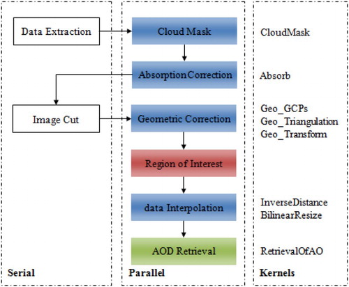
Table 1. Pseudo codes for the parallel procedures.

Procedure	Pseudo codes
Cloud Mask	01: INPUTS: MODIS data of channel 1,3 ,4, 7 and 26 02: for i = 0 to width −1, j = 0 to height −1 do 03: mask with spatial variability with 3*3 window for channel 3 and 26 at (j, i) 04: mask with absolute value of reflectance for channel 3 and 26 at (j, i) 05: union of cloud mask above 06: end for 07: border pixels processing and mask reflectance image with the cloud mask image 08: OUTPUT: reflectance data through cloud mask
Absorption Correction	01: INPUTS: NCEP data, MODIS data 02: initialize gas absorption coefficients and climatology 03: for i = 0 to width*height −1 do 04: match NCEP data with MODIS data 05: calculate gas transmission factors and corrected reflectance 06: end for 07: OUTPUT: reflectance data through absorption correction
Geometric Correction	01: INPUTS: geographic data, uncorrected images 02: for i = 0 to width*height −1 do 03: store GCPs 04: end for 05: for i = 1 to height −1, j = 1 to (width-1)*2 do 06: store triangulation net and calculate affine transformation coefficients 07: end for 08: for i = 1 to height −1, j = 1 to (width-1)*2 do 09 calculate triangulation ranges x_min/max, y_min/max in corrected images 10: for k = y_min to y_max, m = x_min to x_max in corrected images do 11:  if (k,m) in triangulation do 12:  forward calculate coordinates and nearest neighbor re-sampling 13: end for 14: end for 15: OUTPUT: data through geometric correction
Initial Interpolation	01: INPUTS: irregular initial source points 02: for i = 0 to width*height −1 do 03: calculate distances and weights for pixel (i) with all source points 04: re-calculate value of pixel (i) using source points and weights 05: end for 06: for i = 0 to width_roi*height _roi-1 do 07: re-calculate value for pixel (i) using bilinear interpolation method 08: end for 09: OUTPUT: initial images for ROIs
AOD Retrieval	01: INPUTS: corrected reflectance, sensor zenith, solar zenith, initial values 02: for i = 0 to width*height −1 do 03: solve wavelength exponent and Angstrom's turbidity coefficient 04: calculate AOD according to Angstrom's turbidity formula 05: end for 06: OUTPUT: AOD results

2.2. Parallel design consideration

The data extraction and image cut in the left column in Figure 1 are not parallelized, because the data extraction strongly relies on the Geospatial Data Abstraction Library (GDAL) (‘GDAL – Geospatial Data Abstraction Library’, http://www.gdal.org/) HDF4 (‘HDF (4) TOOLS’, http://www.hdfgroup.org/products/hdf4_tools/) and PROJ.4 Cartographic Projections (‘PROJ.4 – Cartographic Projections Library’, http://trac.osgeo.org/proj/) and as the parallel fraction in the image cut is very small. The procedures in blue are supported by both multi-core and GPU parallel options. The determination of ROI shown in red, as it is only multi-core accelerated, this procedure would require a large global memory on the GPU and the parallel fraction is rather small. In addition to the multi-core and GPU version, the AOD retrieval in green is implemented with hybrid patterns to fully utilize the heterogeneous hardware environment simultaneously due to its relatively long runtime. The execution time of the serial workflow was profiled using the data and computing environment in Section 3.1. The overall runtime and the percentage of data input/output (I/O) and calculation are shown in Figures 2 and 3, respectively. The data I/O in this paper refer to the image data read from hard disk and the image data write to hard disk. As shown in Figures 2 and 3, the raw Level 1B data interpolation and AOD retrieval are the most time-consuming parts and have low data I/O fractions, hence are our major concern when optimizing the thread–block configurations in Section 3.3.

Figure 2. Overall serial runtime of all procedures in the retrieval workflow on ‘Ord-System’.

Figure 3. Percentage of data input/output and calculation in serial implementation.

2.3. Parallel implementation for multi-core processors and gpus

Among all procedures in the middle column ‘Parallel’ in Figure 1, the calculation for individual triangulations is independent from each other for the geometric correction, while parallel parts of the other procedures have a pixel-based nature. The ‘for loops’ marked in gray in Table 1 were parallelized either by OpenMP on multi-core processors or by CUDA-C on GPUs.

For multi-core processors, the procedures shown in the middle column ‘Parallel’ in Figure 1 were implemented using OpenMP by parallelizing the according loop(s) through individual pixels or triangulations. The ‘#pragma omp parallel for [collapse (2)]’ directive was used with the advanced scheduling strategy ‘schedule (dynamic)’.

For GPUs, the kernels in the column ‘Kernels’ were created for the procedures in blue and green in Figure 1. Generally, except for the kernels ‘Geo_Triangulation’ and ‘Geo_Transform’ with the workload of one ‘triangulation’ per thread (i.e. the total threads therefore equals the number of triangulations, i.e. (width-1)*(height-1)*2), we assign each thread the workload of processing one ‘pixel’ for all other kernels. The block size is set as two dimensional and was fixed as 16*16 as a starting point. The grid sizes are set dynamically according to the image or triangulation size and the block size. The main techniques conducted specifically for kernels are the following:

• The dynamic shared memory and static shared memory were used in the kernel ‘CloudMask’ and ‘InverseDistance', respectively for sharing data per thread block.

• The ‘#pragma unroll’ was used to unroll a loop within the kernel ‘Absorb’ for less-processing load.

• For ‘Geo_GCPs’, ‘Geo_Triangulation’, ‘Geo_Transform’, data were kept in global memory for the latter kernel after the former kernel finished so that no communication across the PCIe bus to the host memory is necessary among the kernels.

• The ‘atomicExch’ is used to lock a pixel to avoid writing simultaneously to the same global memory address for the kernel ‘Geo_Transform’, as there are overlapping pixels for adjacent triangulations in the corrected images.

• Specifically for the kernel ‘RetrievalOfAOD’ which is time-consuming and our focus for hybrid parallel, a design and implementation benchmarked on Tesla K20 was discussed in an earlier publication (Liu et al. 2015). In this work, the memory of the host is assumed to be large enough to contain all input and output data at once, while the global memory of the GPU is not that large. This is a common situation for workstation computers equipped with a GPU. Hence, the AOD kernel is launched multiple times by dividing the image data according to the limitation of GPU global memory used per launch. The benchmark GPU is equipped with a global memory of 1GB, and additionally uses some memory for rendering and visualization for the connected host system. As many operating systems run watchdog procedures to detect misbehavior in the system and as our calculation kernels are relatively complex, it is necessary to restrict the data amount processed within one kernel launch to make the implementation applicable on a wide range of systems. We limited the data amount to be processed in one kernel launch to 64MB for the GPU implementation, same for the maximum slice size for the hybrid implementation in Sections 2.4 and 3.4. With this assumption, our implementation was executable on several Linux and Windows systems we tested without any further modification in the OS settings.

• The optimization concerning the impact of a two-dimensional thread–block configuration on the runtime was conducted and discussed in Section 3.3.

2.4. Hybrid parallel of multi-core processors and GPUs

In this section, the hybrid parallel implementation based on CUDA and OpenMP is presented for the time-consuming and pixel-based AOD retrieval to enhance the GPU version by utilizing the idling CPU cores.

2.4.1. Static workload distribution

Assuming that the multi-core parallel version for the AOD retrieval obtains an ideal linear speedup compared to the serial implementation, a method presented in Fang et al. (2014) was applied first to distribute the workload between CPU cores and GPU device. Assuming that all CPU cores have the same peak performance, the runtime can be determined with Equation (1). P_gpu and P_cpu represent the theoretical peak performances of the GPU and one CPU core, while is the ratio of workload assigned to the CPU threads gives the total workload, that is, the calculation of overall (height*width) pixels of the image data. The total runtime T is the maximum of the runtime of the workload distributed to CPU T_cpu and that to GPU T_gpu.(1)

The workload distribution is optimal if T_gpu = T_cpu. Nevertheless, the theoretical peak performance cannot be achieved for most real-world codes and mechanisms like caches are not involved in those considerations. To integrate those, the speedup s of the GPU version over a CPU serial one is measured to replace the peak performance ratio P_gpu/P_cpu. As a result, Equation (2) is obtained. In the case that one GPU device is connected to the host, the number of compute threads is m = thread_num-1.(2)

In the following, this method is referred to as ‘Static-1'. However, an ideal linear speedup of the multi-core implementations is still assumed even though it cannot always be achieved in our application due to several reasons, for example, that (1) pixels follow different branches in the program and require different execution runtime, (2) the dynamic OpenMP scheduling causes additional overhead, and (3) we use hyperthreading for 8 threads. Thus, a revised ratio is calculated using existing measurements not only for the GPU speedup but also for the multi-core speedup, resulting in Equation (3). S_cpu and S_gpu represent the speedup of the multi-core and GPU versions obtained by previous measurements. This method is referred to as ‘Static-2' in the following.(3)

Even though it can be expected that the accuracy of the workload estimation increases when more real-test measurements speedups are included in the calculation, the system first of all needs to obtain a prior knowledge of speedups for specific data scenarios under certain computing environments. As we measured, the speedups for different data scenarios vary as, for example, a calculation for an over-sea region takes another branch in the program than over-land regions. Taking the speedups with an over-sea image can therefore lead to strong mispredictions for over-land regions and vice versa. To overcome this drawback and to avoid obtaining a priori knowledge of speedups, we developed a fully automatic and dynamic workload distribution method.

With the two static workload distribution solutions, having calculated the ratio , the first pixels will be assigned to the GPU device, while the rest will be calculated by the m CPU threads. The workload for the GPU device is divided into several batches that fit into the GPU's memory and the calculation kernel is launched several times for regional data after copying the data at once before.

2.4.2. Dynamic workload distribution

Since both static workload distribution methods need existing measurements, a dynamic workload distribution is proposed by dividing the images into slices from the spatial domain. The images are logically divided into slices which consist of one or more lines, and the indexes to these slices are pushed to a task queue. The m = thread_num-1 CPU threads are logically taken as an ‘integrated CPU processor’ as the remaining thread solely serves the GPU on the host side. Every time one task on either the ‘integrated CPU processor’ or the GPU finished, the next task, and therefore the next slice of data, is popped from the top of the task queue and is subsequently assigned to the requesting device. For the GPU, each slice's data are copied to the GPU before its calculation and the results are copied back to the host afterwards as it is just decided at runtime which slice will be processed on which device. The workload distributed to the integrated ‘CPU processor’ is spawned to the m threads.

2.4.3. Hybrid parallel of OpenMP and CUDA-C

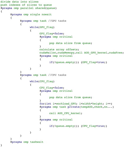
The hybrid pattern was implemented based on CUDA-C and OpenMP. The pseudo codes of parallel implementation for the static and dynamic workload distribution are shown in Figures 4 and 5. The ‘#pragma omp parallel’ defines a parallel region executed by multiple threads in parallel. Inside the parallel region, the ‘#pragma omp single’ specifies that a section of codes for the calculation on the GPU device should be executed on a single thread which is the already mentioned GPU serving thread. The ‘#pragma omp task’ defines a task dynamically which is supported with OpenMP 3.0. The implemented strategy is to let one task be active until all work is done to serve the GPU while a second task itself spawns tasks to serve the remaining CPU cores within the loop iterating over the pixels of the current slice. The ‘#pragma omp critical’ protects the queue so that it can be only accessed by one thread at a time.

Figure 4. Source code segment for the implementation of the static workload distribution.

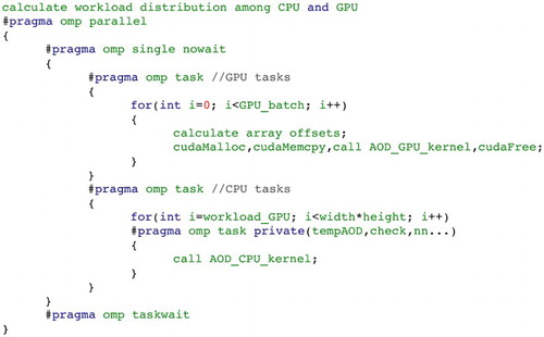
Figure 5. Source code segment for the implementation of the dynamic workload distribution.

3. Results and discussion

3.1. Benchmark data and environment

The benchmark MODIS satellite data were from 1 February 2012 covering 35°E–150°E, 15°N–60°N at 1 km spatial resolution. The MODIS data were downloaded from NASA LAADS web (‘Level 1 and Atmosphere Archive and Distribution System (LAADS Web)’, http://ladsweb.nascom.nasa.gov/).

The workflow was benchmarked on the ‘Ord-System’ shown in Table 2. The serial and multi-core implementations were compiled with the GNU gcc with the ‘-O2’ flag. The GPU implementations were compiled with compute capability 2.0.

Table 2. CPU–GPU configurations for two different compute circumstance.

	‘Ord-System’	‘LoE-System’
CPU configuration	Ubuntu 14.04 LTS	Linux CentOS 6.5
	Intel ® Core ™ i7-960 CPU running at 3.20GHz	Intel ® Core ™ i7-2760QM CPU running at 2.40 GHz
	4 physical cores (hyper-threading activated running 8 logical cores)	4 physical cores (hyper-threading activated running 8 logical cores)
	memory bandwidth: 25.6 GB/s	memory bandwidth: 25.6 GB/s
GPU Configuration	NVIDIA GeForce GTX 460	NVIDIA NVS 4200M
	336 cores	48 cores
	memory: 1GB	memory: 1GB
	memory bandwidth: 115.2 GBsec	memory bandwidth: 12.8 GB/sec

Additionally, the hybrid implementation was evaluated on the LoE-System shown in Table 2. This allows us to show the behavior of the different hybrid approaches for two different system configurations to compare the resulting distribution of workload in Section 3, on one hand on a system (‘Ord-System’) where GPU performs much faster than CPU, and on the other hand on a more biased system with a slightly dominant multi-core processor (‘LoE-System’).

The procedures except the AOD retrieval model solving lead to the same results for all implementations. For the AOD retrieval part, there is relative small and acceptable difference between the C version (for serial and multi-core parallel) and CUDA-C version (for GPU parallel). The accuracy has been analyzed in an earlier publication (Liu et al. 2015).

3.2. Parallel performance for multi-core processors

The calculation runtime, as well as the corresponding speedup for the serial and multi-core implementations, is shown in Table 3. The most time-consuming procedures of the whole workflow, the data interpolation and AOD retrieval, reduce to 308.34s and 324.69s from 1141.02s and 1775.97s, respectively when executed in parallel on the multi-core processor of the ‘Ord-System’. The speedups for the pre-processing and retrieval range from 1.31 to 5.47 with eight threads on this benchmark system with four cores. Excluding the data extraction based on the GDAL library, the multi-core workflow achieves a calculation speedup of 4.09 for the computation steps, and an overall speedup of 3.09 when including the data I/O for intermediate files with eight threads on four physical cores.

Table 3. Calculation performance for the serial, multi-core, and GPU implementations.

	Calculation runtime (s)			Speedup
	Serial	8 Threads	GPU	8 Threads	GPU
Cloud mask	17.31	6.01	1.64	2.88	10.53
Absorption correction	46.37	13.43	1.34	3.45	34.57
Geometric correction	54.11	41.39	12.93	1.31	4.18
Region of interest	17.93	9.83	–	1.82	–
Data interpolation	1141.02	308.34	26.51	3.70	43.03
AOD retrieval	1775.97	324.69	63.70	5.47	27.88
Workflow without data I/O (including image cut in serial)	3110.25	761.21	176.99	4.09	17.57
Workflow with data I/O (including image cut in serial)	3497.64	1133.58	872.82	3.09	4.01

3.3. Parallel performance for GPUs

As an optimization step, the impact of thread–block configuration on the runtime was analyzed. From the serial runtime in Figure 2, it is visible that the data interpolation and AOD retrieval are the most time-consuming parts. As a result, we tuned the two-dimensional thread–block configuration for the data interpolation as a representative for the pre-processing parts and the AOD retrieval separately. The NX and NY dimension of the block size for the pre-processing was varied from 2 to 32, respectively (the maximum possible range due to register limitations without further limiting the register usage per thread); the NX and NY dimension of the block size for the AOD retrieval was, respectively, varied from 2 to 16. The dimensions of grid sizes are again set dynamically according to the overall scene and these block sizes.

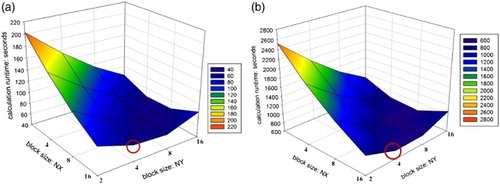
The performance under varying thread–block configurations for the pre-processing and the AOD retrieval on the main benchmark system ‘Ord-System’ is shown in Figures 6 and 7(a). The best performance is achieved executing with 32*8 threads per block for the data interpolation while 16*4 threads per block are optimal for the AOD retrieval.

Figure 6. Thread–block configuration tuning for the pre-processing taking the data interpolation as a representative example. The red circle marks the best thread–block configuration, that is, block size: 32*8 on ‘Ord-System’ leading to the shortest calculation runtime.

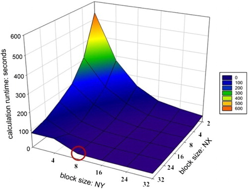
Figure 7. Thread–block configuration for the AOD retrieval. The red circles mark the best thread–block configurations, that is, block size: 16*4 on both ‘Ord-System’ and ‘LoE-System’ leading to the shortest calculation runtime. (a) Ord-System (b) LoE-System.

The benchmark for the GPU version was conducted with the above optimal thread–block configuration. The performance is shown in Table 3 together with the speedups in relation to the serial version. The calculation time reduced from 1141.02s on the CPU (serial) to 26.61s on the GPU for the data interpolation, and from 1775.97s to 63.70s for the retrieval part on our ‘Ord-System’. The lowest calculation speedup gained by the GPU implementation is 4.18 for the geometric correction, while the GPU gained higher speedups from 10.53 to 43.03 for the other procedures compared to the original serial C counterpart. The calculation speedup is 17.57 for the computational steps of the whole workflow, while also including the data I/O for intermediate files the overall speedup is 4.01. The runtime performance reduction of the overall workflow when including the data I/O results from (1) the data I/O procedures are called from the GDAL library with varying performance in our tests, (2) some big image data need to be split into smaller images to be performed on GPUs with a rather limited memory for the ‘Ord-System’, therefore increasing the data I/O calls. Additionally, the speedup reduction when including data I/O is based on the fact that the relative amount of data I/O is much higher for the GPU implementation than for the CPU as the GPU kernel speedup is accordingly large.

3.4. Hybrid parallel performance analysis

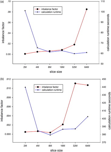
The optimal thread–block configuration for the ‘LoE-System’ was obtained as well and turned out to be the same than for the ‘Ord-System’ shown in Figure 7(b). To test the impact of slice size (i.e. the bytes taken by a slice) on the performance and find a slice size that leads to the best performance, the slice size of the dynamic hybrid implementation was varied from 2MB to 64MB. The impacts of slice size on the imbalance factor and calculation runtime are shown in Figure 8. The imbalance factor is defined as the runtime ratio of max (CPU, GPU)/ min (CPU, GPU)-1, and thus the calculation is well balanced if this imbalance factor is small. The smaller the slice size, the more balanced is the overall workload distribution as the portions of work are smaller and can be spawned until both devices finish almost simultaneously. However, this comes at a price as the dynamic distribution through the queue causes an overhead for each pop operation on the task queue. The goal is to find the slice size resulting in the shortest runtime by balancing the advantage of small slices for a small imbalance factor with the drawback of the overhead for accessing the queue more often. In our case, the fastest overall runtime of 59.73s was achieved using 32MB slices on the ‘Ord-System’ and 8MB with 379.38s on the ‘LoE-System’. Within 4MB and 16MB, the differences in terms of resulting runtime are moderate for both systems.

Figure 8. Slice size impacts on the imbalance factor and calculation runtime. As the imbalance factor is defined as the runtime ratio of ‘max(CPU, GPU)/min(CPU, GPU)-1’, the calculation is well balanced if this imbalance factor is small. (a) Ord-System. (b) LoE-System.

A comparison of the calculation runtime for the presented static and hybrid parallel implementations as well as for the single thread, multi-thread, and GPU version on the main benchmark system (‘Ord-System’) and on the ‘LoE-System’ is shown in Figure 9. The imbalance factor represents the difference of GPU and CPU runtimes within the hybrid code versions. As already mentioned, Static-1 and Static-2 are the static parallel distributions supposing an ideal linear speedup of the multi-core version in the first case and known speedups for both multi-core and GPU versions in the second case. It can be seen in Figure 9 that both static versions are by far not balanced on the ‘Ord-System’ while the dynamic hybrid scheduling theme reaches an almost perfect balance of workload between CPU and GPU. On the ‘Ord-System’ the calculation runtimes are 127.59s, 84.74s, and 59.73s for the three hybrid patterns. Compared to the runtimes of 324.69s and 63.70s for the multi-core version with 8 threads and GPU version in Table 3, the two static patterns are faster than the multi-core one, however slower than the pure GPU version. The dynamic hybrid version outperforms the GPU implementation just a little bit.

Figure 9. Comparison of balance and calculation runtime for two static and one hybrid implementation patterns. No GPU is in use for the serial (1 thread) and the multi-core parallel with 8 threads. The GPU time in the GPU parallel and three hybrid parallel versions include the computation on GPU and communication between GPU and the corresponding CPU host thread. (a) Ord-System. (b) LoE-System.

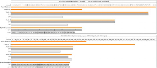
To find the source of those effects, Figure 10 presents details about how the slices are scheduled among CPU and GPU (for better readability the figures show the scheduling for only half of the whole scene). It is noticeable that, on the ‘Ord-System’, the CPU only gets a very little number (<10%) of the (in pixels) equally sized slices with the dynamic implementation. This is anyway not surprising, as the pure GPU version is at a comparable factor faster than the pure multi-core version. As the dynamic hybrid scheduling pattern can only pass a very small amount of work to the CPU for concurrent calculations on CPU and GPU and additionally introduces an overhead due to the task queue operations, the advantage of the hybrid dynamic version is only very small compared to the outstandingly well-performing GPU version on the ‘Ord-System’. The results for the static versions show that the estimation of the CPU's and GPU's performance lead to a strong imbalance in the final distribution of work for the two approaches even though the more precise Static-2 performs better than Static-1. On the ‘LoE-System’ instead, the GPU's and the CPU's performances are more similar for our application. As a result, the dynamic hybrid version distributes an almost equal number of slices to the GPU and the CPU and the resulting runtime is distinctly faster than both pure CPU and GPU approaches and also than the two static versions. This shows that the dynamic hybrid scheduling pattern (a) works well for balanced (in terms of CPU–GPU performance) as well as for unbalanced systems and that it can (b) naturally gain more additional performance (compared to the pure versions) by concurrent calculations on CPU and GPU on a balanced system. Figure 10 additionally shows how the different regions of the scene (e.g. over-sea and over-land) influence the workflow and therefore the runtime of a single slice. Approximately in the vertical middle of the image, the slices’ runtimes become very small even though each slice calculated the same amount of pixels.

Figure 10. Workload and slice comparison of the different approaches applied on half of the image (for better readability). The bars in orange show the runtime of different implementations. For the three hybrid parallel versions, the runtime of workload distributed to CPU and GPU are presented in dark and light gray, respectively. For the dynamic hybrid parallel version, the slice number and corresponding runtime are presented.

Summarizing one can say that the hybrid pattern makes full use of idling CPU cores while computing on GPUs on both tested systems and that the performance of the dynamic hybrid parallel version compared to the GPU and CPU versions relates to the dominance of either the GPU device or the CPU.

4. Conclusion and future work

This article presented an efficient AOD retrieval workflow from MODIS data based on multi-core processors and GPU accelerators. The multi-core implementation gained a best speedup of 5.47 with 8 threads on our main benchmark system with 4 physical cores. Concerning the different parts of overall workflow, the GPU version obtained a smallest speedup of 4.18 for the geometric correction and higher speedup from 10.53 to 43.03 for the other procedures. To fully utilize idling CPU cores while computing on GPU, the hybrid parallel implementations considering static and dynamic distribution methods have been developed to enhance the time-consuming and pixel-based AOD retrieval and they have been evaluated on two different system types, a Ord-System and a LoE-System. Our developed dynamic hybrid scheduling pattern shows advantages by reducing the workload imbalance and the calculation runtime compared to pure multi-core CPU and GPU approaches as well as compared to static hybrid approaches. Nevertheless, when computing in a desktop workstation or server system with a powerful GPU device, the pure GPU implementation will in general be the better choice.

A remarkable amount of time in the pre-processing was consumed with data I/O from data extraction using libraries GDAL, HDF4, and PROJ.4 and files read/write for the intermediate files for processing steps. With the parallel implementations of the calculation fractions inside these pre-processing steps, the data I/O becomes a bottleneck. The data I/O for the intermediate files reduced the overall speedup of the workflow computation steps from 17.57 to 4.01 for GPU, and from 4.09 to 3.09 for multi-core processors. In future research, the intermediate files of the processing steps could be kept in memory if the available system has memory larger than 8GB. Thus the overall speedups are expected to approach the calculation speedups. A parallel solution of extracting data from HDF file is also desired. In addition, deploying the workflow in a GPU cluster and scheduling workflow modules among multiple CPU and GPU computing resources is one further step.

Acknowledgement

This work was supported in part by the National Natural Science Foundation of China (NSFC) under Grant 41271371 and Grant 41471306, the Major International Cooperation and Exchange Project of NSFC under Grant 41120114001, the Institute of Remote Sensing and Digital Earth Institute, Chinese Academy of Sciences (CAS-RADI) Innovation project under Grants Y3SG0300CX, the graduate foundation of CAS-RADI under Grant Y4ZZ06101B, and the Joint Doctoral Promotion Program hosted by the Fraunhofer Institute and Chinese Academy of Sciences. Many thanks are due to the Fraunhofer Institute for Algorithms and Scientific Computing SCAI for the multi-core and GPU platform used in this paper.

Disclosure statement

No potential conflict of interest was reported by the authors.

References

- Abouali, Mohammad, Joris Timmermans, Jose E. Castillo, and Bob Z. Su. 2013. “A High Performance GPU Implementation of Surface Energy Balance System (SEBS) Based on CUDA-C.” Environmental Modelling & Software 41: 134–138. doi: 10.1016/j.envsoft.2012.12.005
- Bernabe, Sergio, Sebastián López, Antonio Plaza, and Roberto Sarmiento. 2013. “GPU Implementation of An Automatic Target Detection and Classification Algorithm for Hyperspectral Image Analysis.” Ieee Geoscience And Remote Sensing Letters 10 (2): 221–225. doi: 10.1109/LGRS.2012.2198790
- Christophe, Emmanuel, Julien Michel, and Jordi Inglada. 2011. “Remote Sensing Processing: From Multicore to GPU.” IEEE Journal of Selected Topics in Applied Earth Observations and Remote Sensing 4 (3): 643–652. doi: 10.1109/JSTARS.2010.2102340
- Fang, Liuyang, Mi Wang, Deren Li, and Jun Pan. 2014. “CPU/GPU Near Real-Time Preprocessing for ZY-3 Satellite Images: Relative Radiometric Correction, MTF Compensation, and Geocorrection.” ISPRS Journal of Photogrammetry and Remote Sensing 87: 229–240. doi: 10.1016/j.isprsjprs.2013.11.010
- Fu, Bitao, Cheng Wang, and Qiuwen Zhang. 2005. “Parallel Algorithm of Geometrical Correction for MODIS Data Based on Triangulation Network.” Paper presented at the 2005 IEEE International Geoscience and Remote Sensing Symposium, Seoul, Korea, 25–29 July 2005.
- "GDAL - Geospatial Data Abstraction Library." http://www.gdal.org/.
- Gonzalez, Carlos, Sergio Sánchez, Abel Paz, Javier Resano, Daniel Mozos, and Antonio Plaza. 2013. “Use of FPGA or GPU-based Architectures for Remotely Sensed Hyperspectral Image Processing.” Integration, the VLSI Journal 46 (2): 89–103. doi: 10.1016/j.vlsi.2012.04.002
- Goodchild, Michael F, Huadong Guo, Alessandro Annoni, Ling Bian, Kees de Bie, Frederick Campbell, Max Craglia, Manfred Ehlers, John van Genderen, and Davina Jackson. 2012. “Next-generation Digital Earth.” Proceedings of the National Academy of Sciences 109 (28): 11088–11094. doi: 10.1073/pnas.1202383109
- GU, Ling-jia, Rui-zhi Ren, and Hao-feng Wang. 2010. “MODIS Imagery Geometric Precision Correction Based on Longitude and Latitude Information.” The Journal of China Universities of Posts and Telecommunications 17: 73–78. doi: 10.1016/S1005-8885(09)60603-8
- Guo, Huadong. 2015. “Big Data for Scientific Research and Discovery.” International Journal of Digital Earth 8 (1): 1–2. doi: 10.1080/17538947.2015.1015942
- Guo, Wei, JianYa Gong, WanShou Jiang, Yi Liu, and Bing She. 2010. “OpenRS-Cloud: A Remote Sensing Image Processing Platform Based on Cloud Computing Environment.” Science China Technological Sciences 53 (1): 221–30. doi: 10.1007/s11431-010-3234-y
- "HDF (4) TOOLS." http://www.hdfgroup.org/products/hdf4_tools/
- IPCC. 2013. “Climate Change 2013: The Physical Science Basis. Contribution of Working Group I to the Fifth Assessment Report of the Intergovernmental Panel on Climate Change.” In edited by T. F. Stocker, D. Qin, G.-K. Plattner, M. Tignor, S. K. Allen, J. Boschung, A. Nauels, Y. Xia, V. Bex, and P. M. Midgley. Cambridge: Cambridge University Press.
- Kim, Ick-Hoi, and Ming-Hsiang Tsou. 2013. “Enabling Digital Earth Simulation Models Using Cloud Computing or Grid Computing–Two Approaches Supporting High-performance GIS Simulation Frameworks.” International Journal of Digital Earth 6 (4): 383–403. doi: 10.1080/17538947.2013.783125
- Lee, Craig A., Samuel D. Gasster, Antonio Plaza, Chein-I Chang, and Bormin Huang. 2011. “Recent Developments in High Performance Computing for Remote Sensing: A Review.” IEEE Journal of Selected Topics in Applied Earth Observations and Remote Sensing 4 (3): 508–527. doi: 10.1109/JSTARS.2011.2162643
- Levy, R. C., S. Mattoo, L. A. Munchak, L. A. Remer, A. M. Sayer, F. Patadia, and N. C. Hsu. 2013. “The Collection 6 MODIS Aerosol Products Over Land and Ocean.” Atmospheric Measurement Techniques 6 (11): 2989–3034. doi: 10.5194/amt-6-2989-2013
- "Level 1 and Atmosphere Archive and Distribution System (LAADS Web)." http://ladsweb.nascom.nasa.gov/.
- Liu, Jia, Dustin Feld, Yong Xue, Jochen Garcke, and Thomas Soddemann. 2015. “Multi-core Processors and Graphics Processing Unit Accelerators for Parallel Retrieval of Aerosol Optical Depth from Satellite Data: Implementation, Performance and Energy Efficiency.” IEEE Journal of Selected Topics in Applied Earth Observations and Remote Sensing 8 (5): 2306–2317. doi: 10.1109/JSTARS.2015.2438893
- Lohmann, Ulrike, and Johann Feichter. 2005. “Global Indirect Aerosol Effects: A Review.” Atmospheric Chemistry and Physics 5 (3): 715–737. doi: 10.5194/acp-5-715-2005
- Luo, Yuxiang, Xiaobo Zheng, Tianliang Zhao, and Juan Chen. 2014. “A Climatology of Aerosol Optical Depth Over China from Recent 10 Years of MODIS Remote Sensing Data.” International Journal of Climatology 34 (3): 863–870. doi: 10.1002/joc.3728
- Nickolls, John, and William J. Dally. 2010. “The GPU Computing Era.” IEEE Micro 30 (2): 56–69. doi: 10.1109/MM.2010.41
- Parker, J. Anthony, Robert V. Kenyon, and D. Troxel. 1983. “Comparison of Interpolating Methods for Image Resampling.” IEEE Transactions on Medical Imaging 2 (1): 31–39. doi: 10.1109/TMI.1983.4307610
- Paz, Abel, and Antonio Plaza. 2010. “Clusters Versus GPUs for Parallel Target and Anomaly Detection in Hyperspectral Images.” EURASIP Journal on Advances in Signal Processing 2010.
- Plaza, Antonio, Qian Du, Yang-Lang Chang, and Roger L. King. 2011. “High Performance Computing for Hyperspectral Remote Sensing.” IEEE Journal of Selected Topics in Applied Earth Observations and Remote Sensing 4 (3): 528–544. doi: 10.1109/JSTARS.2010.2095495
- "PROJ.4 - Cartographic Projections Library." http://trac.osgeo.org/proj/.
- Remer, Lorraine A., Richard G. Kleidman, Robert C. Levy, Yoram J. Kaufman, Didier Tanré, Shana Mattoo, J. Vanderlei Martins, et al. 2008. “Global Aerosol Climatology from the MODIS Satellite Sensors.” Journal of Geophysical Research: Atmospheres 113 (D14S07): 1–18.
- Savtchenko, A., D. Ouzounov, S. Ahmad, J. Acker, G. Leptoukh, J. Koziana, and D. Nickless. 2004. “Terra and Aqua MODIS Products Available from NASA GES DAAC.” Advances in Space Research 34 (4): 710–4. doi: 10.1016/j.asr.2004.03.012
- Su, Xiang, Jiaji Wu, Bormin Huang, and Zhensen Wu. 2013. “GPU-Accelerated Computation for Electromagnetic Scattering of a Double-Layer Vegetation Model.” IEEE Journal of Selected Topics in Applied Earth Observations and Remote Sensing 6 (4): 1799–1806. doi: 10.1109/JSTARS.2012.2219508
- Wolfe, Robert E., David P. Roy, and Eric Vermote. 1998. “MODIS Land Data Storage, Gridding, and Compositing Methodology: Level 2 Grid.” IEEE Transactions on Geoscience and Remote Sensing 36 (4): 1324–1338. doi: 10.1109/36.701082
- Xu, Wen. 2012. “The Application of China's Land Observation Satellites within the Framework of Digital Earth and Its Key Technologies.” International Journal of Digital Earth 5 (3): 189–201. doi: 10.1080/17538947.2011.647774
- Xue, Yong, Jianwen Ai, Wei Wan, Huadong Guo, Yingjie Li, Ying Wang, Jie Guang, Linlu Mei, and Hui Xu. 2011. “Grid-enabled High-performance Quantitative Aerosol Retrieval from Remotely Sensed Data.” Computers & Geosciences 37 (2): 202–206. doi: 10.1016/j.cageo.2010.07.004
- Xue, Yong, and A. P. Cracknell. 1995. “Operational Bi-angle Approach to Retrieve the Earth Surface Albedo from AVHRR Data in the Visible Band.” International Journal of Remote Sensing 16 (3): 417–429. doi: 10.1080/01431169508954410
- Xue, Yong, Xingwei He, Hui Xu, Jie Guang, Jianping Guo, and Linlu Mei. 2014. “China Collection 2.0: The Aerosol Optical Depth Dataset from the Synergetic Retrieval of Aerosol Properties Algorithm.” Atmospheric Environment 95: 45–58. doi: 10.1016/j.atmosenv.2014.06.019
- Xue, Yong, Dominic Palmer-Brown, and Huadong Guo. 2011. “The Use of High-performance and High-throughput Computing for the Fertilization of Digital Earth and Global Change Studies.” International Journal of Digital Earth 4 (3): 185–210. doi: 10.1080/17538947.2010.535569
- Yang, Chaowei, Yan Xu, and Douglas Nebert. 2013. “Redefining the Possibility of Digital Earth and Geosciences with Spatial Cloud Computing.” International Journal of Digital Earth 6 (4): 297–312. doi: 10.1080/17538947.2013.769783