Global land mapping of satellite-observed CO₂ total columns using spatio-temporal geostatistics

ABSTRACT

This study presents an approach for generating a global land mapping dataset of the satellite measurements of CO₂ total column (XCO₂) using spatio-temporal geostatistics, which makes full use of the joint spatial and temporal dependencies between observations. The mapping approach considers the latitude-zonal seasonal cycles and spatio-temporal correlation structure of XCO₂, and obtains global land maps of XCO₂, with a spatial grid resolution of 1° latitude by 1° longitude and temporal resolution of 3 days. We evaluate the accuracy and uncertainty of the mapping dataset in the following three ways: (1) in cross-validation, the mapping approach results in a high correlation coefficient of 0.94 between the predictions and observations, (2) in comparison with ground truth provided by the Total Carbon Column Observing Network (TCCON), the predicted XCO₂ time series and those from TCCON sites are in good agreement, with an overall bias of 0.01 ppm and a standard deviation of the difference of 1.22 ppm and (3) in comparison with model simulations, the spatio-temporal variability of XCO₂ between the mapping dataset and simulations from the CT2013 and GEOS-Chem are generally consistent. The generated mapping XCO₂ data in this study provides a new global geospatial dataset in global understanding of greenhouse gases dynamics and global warming.

KEYWORDS:

• XCO₂
• ACOS-GOSAT
• Spatio-temporal geostatistics
• global mapping
• geospatial dataset

1. Introduction

The concentration of atmospheric carbon dioxide (CO₂), the most important anthropogenic greenhouse gas, has increased by 40% since pre-industrial times as a result of the burning of fossil fuels, cement production and deforestation (IPCC 2013). While the surface carbon dioxide monitoring network (e.g. GLOBALVIEW-CO₂) provides in situ measurements of CO₂, the spatio-temporal variability and distribution of CO₂ sources and sinks are still not fully understood mainly due to the sparseness and spatial inhomogeneity of the network (Heimann 2009; Ciais et al. 2014). Satellite observations of CO₂ columns, because of their global coverage and high measurement density, can complement the surface network and be used to advance our understandings of the carbon cycle and its changes (Duren and Miller 2012; McKain et al. 2012). The Japanese Greenhouse gases Observation SATellite (GOSAT), the world's first spacecraft dedicated to quantify the atmospheric CO₂ and methane concentrations, was successfully launched in 2009 (Yokota et al. 2009). The Atmospheric CO₂ Observations from Space (ACOS) project team from NASA's Orbiting Carbon Observatory (OCO) applied the OCO calibration, validation and remote sensing retrieval algorithm to analyze the GOSAT Level 1B data products, and obtain the column-averaged CO₂ dry air mole fraction (XCO₂) data products (Wunch et al. 2011a; O'Dell et al. 2012). These ACOS retrievals from GOSAT are hereafter referred to as ACOS-GOSAT. Other satellite instruments, including SCIAMACHY (Bovensmann et al. 1999) and OCO-2 (Crisp et al. 2004; Boesch et al. 2011), and the forthcoming CarbonSAT (Bovensmann et al. 2010) and TanSAT (Liu, Yang, and Cai 2013), are also aiming at measuring global greenhouse gases. As more data from these satellites are becoming available, global analysis of XCO₂ by applying methods for data modeling, validation and comparison, ranging from simple spatial and temporal averaging to sophisticated data assimilation approaches, have become possible (e.g. Buchwitz et al. 2005; Schneising et al. 2008, 2011, 2014; Katzfuss and Cressie 2011; Morino et al. 2011; Wunch et al. 2011b; Buchwitz et al. 2013; Reuter et al. 2013).

However, due to constraints such as cloud coverage and GOSAT Fourier Transform Spectrometers (FTS) observation mode (NIES GOSAT Project 2010), the number of available GOSAT XCO₂ retrievals is largely reduced and irregularly distributed in space and time, which make it difficult to directly interpret their scientific significance without further data analysis. Furthermore, the large gaps between satellite observations provide a challenge for study areas with insufficient data (Kort et al. 2012). One solution is the development of a statistical mapping method, which generates a regular distribution map of XCO₂ from the irregular observations, to improve the spatio-temporal coverage. This mapping dataset can potentially provide us a new way to evaluate the roles of anthropogenic emissions (sources) on atmospheric CO₂ enhancement and biospheric activities (sinks) on global CO₂ seasonal cycle. As shown in Keppel-Aleks, Wennberg, and Schneider (2011, 2012), the total column carbon dioxide XCO₂ retrieved from satellite has a larger footprint than conventional surface data because the column data are a combination of not only boundary layer CO₂ but also free troposphere CO₂. Therefore, variations in XCO₂ are primarily determined by large-scale flux patterns. As a result, significant correlation exits between XCO₂ data (Keppel-Aleks, Wennberg, and Schneider 2011). Therefore, a geostatistical approach (Cressie 1993; Cressie and Wikle 2011), which uses the inherent autocorrelation between satellite-observed XCO₂ data to make optimal predictions and is flexible in handling irregular datasets, can be exploited to meet the requirements of filling gaps and mapping XCO₂ at high spatio-temporal resolution.

The mapping of satellite observations of XCO₂ has been investigated in several studies from different perspectives (Hammerling, Michalak, and Kawa 2012; Nguyen et al. 2014a; Zeng et al. 2014). Spatial-only kriging, a conventional geostatistical method, was widely adopted to generate the XCO₂ mapping data products (Tomosada et al. 2008, 2009; Liu et al. 2012; Watanabe et al. 2015). Hammerling, Michalak, and Kawa (2012; Hammerling et al. 2012) and Tadić et al. (2014) extended the spatial-only kriging method to a global scale using a moving window technique. This conventional spatial-only geostatistical method, which only makes use of spatial correlation, does not take into account the temporal correlation structure of the CO₂ data, and therefore the dynamic CO₂ temporal variations including the annual increase and seasonal cycles (WMO 2014; Schneising et al. 2014) are not fully considered. By incorporating the temporal variability of XCO₂, Zeng et al. (2013, 2014) extended this method into the spatio-temporal domain to generate XCO₂ maps at high spatio-temporal resolution, and illustrated the effectiveness of the method by applying it to China as a study region. The advantages of this spatio-temporal geostatistical approach lie in (1) the utilization of the joint spatial and temporal dependences between observations to provide a probabilistic framework for data analysis and prediction and (2) inclusion of a larger dataset in both space and time to support stable parameter estimation and prediction (Cressie and Wikle 2011; De Iaco and Posa 2012).

Building on the regional mapping method using spatio-temporal geostatistics developed by Zeng et al. (2014), this study aims to develop a global land mapping method for the ACOS-GOSAT XCO₂ dataset. However, the extension from the regional method to the global case is not straightforward, since the assumptions of a uniform spatio-temporal trend and spatio-temporal correlation structure in the regional dataset are often violated in the global case. As a solution, we use the long-term CarbonTracker CT2013 XCO₂ data and global annual CO₂ growth rate calculated from surface observation sites to construct the spatio-temporal deterministic trend of XCO₂, including latitude-zonal seasonal cycle and global annual increase, and then remove the trend from the ACOS-GOSAT data. The correlation structures of the XCO₂ data are then calculated and modeled for each latitude zone. Finally, the spatio-temporal geostatistical prediction approach is implemented to obtain the global land mapping of XCO₂, and quantify the corresponding prediction uncertainties. The resulting dataset is assessed in three ways. First, a cross-validation technique (Arlot 2010) for accuracy assessment of statistical models is applied to assess the prediction accuracy of this mapping approach. Second, a comparison with Total Carbon Column Observing Network (TCCON) data is performed to validate the mapping results at global TCCON sites. Finally, we investigate the similarities and discrepancies between the mapping dataset and model XCO₂ calculations from both CarbonTracker CT2013 and GEOS-Chem by comparing their spatio-temporal variations. As suggested by Hammerling, Michalak, and Kawa (2012), the mapping dataset will provide a useful complement to studies of carbon flux inversion with modeled CO₂ fields generated by carbon flux estimates coupled with an atmospheric transport model.

Production of global geospatial data plays a key role in supporting the development of digital earth (Guo, Liu, and Zhu 2010), and application of these global geospatial data in global change research has been an important goal for ‘Digital Earth’ (Shupeng and van Genderen 2008). Our study contributes to these two topics by demonstrating (1) how to effectively and precisely produce a global geospatial dataset of CO₂ column distribution at high spatio-temporal resolution and (2) how these data can be used to analyze the spatio-temporal variations of CO₂. The mapping approach developed in this study can be further incorporated with ‘Digital Earth’ framework for geospatial data production in diverse global change studies.

In Section 2, we provide a description of the data from satellite, ground observation and model simulations used in this paper. We then introduce the basic theories of spatio-temporal geostatistics, and the global land mapping approach in Section 3. The results of applying the approach are illustrated and discussed in Section 4, and conclusions follow in Section 5.

2. Data

2.1. ACOS-GOSAT data product

The v3.3 ACOS-GOSAT XCO₂ data, spanning from 1 June 2009 to 15 May 2013, are used in this study. Because of some potential deficiencies identified in land median-gain and ocean glint retrievals (Nguyen et al. 2014b), only the land high-gain data are used. In comparison with the TCCON, the v3.3 data show a mean global bias of about 1.34 ppm and a standard deviation of 1.83 ppm (ACOS Data User's Guide 2014). Following the data user guide, data filtering and bias correction are carried out before the following science analysis.

The mapping dataset has a temporal resolution of 3 days determined by the GOSAT 3-day orbiting period. Therefore, in this study, we set the basic time-unit to be 3 days. In general, there are nearly 122 time-units in 1 year (365/3 ≈ 122), and from 1 June 2009 to 15 May 2013, 483 time-units of ACOS-GOSAT v3.3 data are used in this study. The basic statistics for the XCO₂ data used each year are listed in Table 1. The standard deviations for the four years are almost the same, while the annual mean value increases steadily, with an average annual increase of 2.03 ppm, which is in good agreement with the global mean annual increase of about 2 ppm from the GLOBALVIEW surface in situ flask network (WMO 2014; Wunch et al. 2011b). Figure 1 shows the monthly global distribution of the ACOS-GOSAT XCO₂ retrievals, taking four months (July 2009, October 2009, January 2010 and April 2010) in four different seasons for the first year of ACOS-GOSAT measurements as examples. The study area of global land region for mapping covers land regions between 40°S and 70°N, as shown in gray in Figure 3. It can be inferred from Figure 1 that the satellite retrievals are irregularly distributed globally, and the available retrievals also change with observation time. Large gaps between satellite observations can be found in some key regions, such as over the forests in southern China, where net ecosystem production is high but there are few satellite observations in summer, mainly due to the frequent cloudy weather. Figure 2 shows the spatial distribution and temporal variation of the number of available satellite observations after data filtering. The numbers of retrievals are irregularly distributed in both space and time. As shown in Figure 2(a), it can be seen that the number of retrievals is greater over the southern regions of South America, North America and Africa, as well as over Central Eurasia and Australia. However, data over northern Africa (around the Sahara desert) and parts of the central Australia, where data are measured with median-gain (Crisp et al. 2012), are excluded by the data-filtering approach. From Figure 2(b), the largest number of measurements is available around August and smallest around January, with an obvious annual cycle.

Figure 1. Example of the spatial distribution and variation of the used ACOS-GOSAT XCO₂ retrievals for four months of (a) July 2009, (b) October 2009, (c) January 2010 and (d) April 2010 over global land.

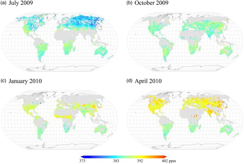
Figure 2. (a) Global spatial distribution density of the used ACOS-GOSAT XCO₂ retrievals (after filtering) from June 2009 to May 2013 in terms of available data number in grids of 5°longitude by 5°latitude and (b) temporal variation of available ACOS-GOSAT retrievals (after filtering) in each 3-day interval. The dashed rectangle area in (a) from 5 to 15°N and 20°W to 40°E covers the tropical region in central Africa, which will be used in Sections 4.5 and 4.6.

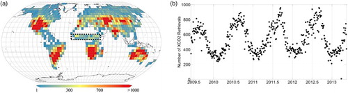
Table 1. Annual statistics for the ACOS-GOSAT v3.3 XCO₂ global land data used in this study after filtering and bias-correction.

	Number of retrievals	Minimum (ppm)	Maximum (ppm)	Mean (ppm)	Standard deviation (ppm)
June 2009–May 2010	58,437	355.89	403.65	386.73	3.11
June 2010–May 2011	67,840	375.72	406.60	389.01	2.92
June 2011–May 2012	67,987	357.58	404.66	390.73	2.94
June 2012–May 2013	65,360	378.92	408.14	392.82	2.95

2.2. The total carbon column observing network

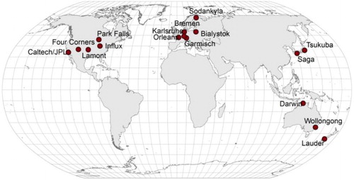
The TCCON, a global network of ground-based FTS established for the validation of near-infrared total column measurements from satellite observations (Wunch et al. 2011b; see TCCON Data Access in the references for details), is collected for the validation of the global land mapping dataset. Based on comparisons with integrated aircraft profiles, TCCON has a high accuracy of approximately 0.25% in XCO₂ (Wunch et al., 2011a). The TCCON data have been used to calibrate the ACOS-GOSAT retrievals (Wunch et al. 2011a). In this study, the 2012 release version of the TCCON data (‘GGG2012’) for 16 sites is used. For each TCCON site, we use all available data within the period from June 2009 to May 2013. Figure 3 shows the spatial distribution of the TCCON sites used in this study. More detailed information about the TCCON sites is given in Table 4 in Section 4.4. TCCON sites at high north latitudes (>70°N) and the ocean are not considered in this study.

Figure 3. Global distribution of the 16 TCCON sites used for the comparison with the mapping dataset, and the global land study area for mapping in gray.

2.3. CarbonTracker CT2013 and GEOS-Chem model calculations of XCO₂

Both the XCO₂ data from CarbonTracker CT2013 and the GEOS-Chem model are used in this study, in order to investigate the similarities and differences between the global land mapping dataset and the modeled XCO₂ and provide potential evidences for further improvement of the satellite retrievals and model simulations.

2.3.1. CarbonTracker CT2013 XCO₂ dataset

CarbonTracker is a modeling system for atmospheric CO₂ developed by the National Oceanic and Atmospheric Administration (NOAA). Coupled with an atmospheric transport model, CarbonTracker assimilates global atmosphere CO₂ observations from ground surface air samples, tall tower and aircrafts to simulate the global CO₂ distribution and to track global CO₂ sources and sinks (Peters et al. 2007). The 2013 release of CarbonTracker, CT2013, combines observations and flux estimates through the end of 2012 to produce estimates of global atmospheric CO₂ and surface-atmosphere fluxes from January 2000 to December 2012 (see CarbonTracker CT2013 Data Access in the references for details). The model produces regularly gridded CO₂ at a spatial resolution of 2° in latitude by 3° in longitude with 25 vertical levels before 2006 and 34 vertical levels after 2006, and with a high temporal resolution of 3 hours. CarbonTracker is widely used in analyzing global CO₂ with satellite observations (e.g. Schneising et al. 2008, 2014; Nguyen et al. 2014b). In this study, we use the long-term CT2013 data from January 2000 to December 2012 to model the deterministic spatio-temporal trend of XCO₂. Besides, we use the CT2013 data from June 2009 to December 2012 for comparison with the original satellite retrievals and the corresponding mapping dataset. The CO₂ profile data from the model are transformed to CO₂ dry air mole fractions, XCO₂, by using the pressure-averaged method described by Connor et al. (2008).

2.3.2. GEOS-Chem XCO₂ dataset

The GEOS-Chem model (http://geos-chem.org) is a global 3-D chemical transport model for simulating atmospheric composition using assimilated meteorological inputs from the Goddard Earth Observing System (GEOS-5) of the NASA Global Modeling and Assimilation Office. A recent update of the atmospheric CO₂ simulations using GEOS-Chem was developed by Nassar et al. (2010). GEOS-Chem is widely used in analyzing global CO₂ with satellite observations (e.g. Feng et al. 2009; Cogan et al. 2012). Deng et al. (2014) employed the GEOS-Chem four-dimensional variational (4D-Var) data assimilation system to assimilate ACOS-GOSAT XCO₂ from June 2009 to December 2010 for quantifying monthly and regional estimates of CO₂ fluxes for the year 2010. In this study, we used the a posteriori atmospheric CO₂ distributions from Deng et al. (2014), which were produced by assimilating ACOS-GOSAT v2.10 data at a horizontal resolution of 4° by 5°. Only the data for 2010 are available in this study. The CO₂ profiles from the a posteriori GEOS-Chem simulation were transformed to XCO₂ using the pressure-averaged method described by Connor et al. (2008).

3. Methodologies

As an extension of spatial geostatistics, the application of spatio-temporal geostatistics in data analysis has become common in recent years (Cressie and Wikle 2011; De Iaco and Posa 2012). Zeng et al. (2014) proposed the use of spatio-temporal geostatistics in generating regional satellite-observed XCO₂ maps at high spatio-temporal resolution, and illustrated the method by applying it to the study area of China. However, extending this regional spatio-temporal geostatistical approach to the global land case is not straightforward, since the regional approach depends on uniform spatio-temporal trends and spatio-temporal correlation structures in the regional dataset. This assumption for global XCO₂ is often violated, as shown by Alkhaled et al. (2008). Instead of assuming a uniform trend as in the regional study, in this study we construct the spatio-temporal trend of XCO₂, including latitude-zonal seasonal cycle and global annual increase, by incorporating precise ground-based observations and model simulated data, which are shown to have well-reproduced large-scale features of the atmospheric CO₂ distribution (Cogan et al. 2012). We use the NOAA Earth System Research Laboratory (ESRL) global annual CO₂ growth rate (Conway and Tans 2015) to determine the annual increase of XCO₂ as in Wunch et al. (2013), and fit the CT2013 XCO₂ time series in each latitude band using a set of annual harmonic functions to construct the latitude-zonal seasonal cycle. After detrending the data by excluding the modeled trend to get the residual dataset, we then calculate the spatio-temporal correlation structures between XCO₂ data in each 10° latitude zone since the variations in XCO₂ are similar zonally (Wunch et al. 2011a; Schneising et al. 2014). Finally, the space–time kriging with a moving flexible kriging neighborhood (Haas 1995) is implemented to obtain the global land maps of XCO₂. A brief introduction of spatio-temporal geostatistics is furnished in this section, followed by an introduction of the global land mapping approach for the ACOS-GOSAT XCO₂ data. The spatial-only method, as a comparison with spatio-temporal method, is also briefly introduced.

3.1. Spatio-temporal geostatistics for global land mapping

3.1.1. Spatio-temporal random field model

In spatio-temporal geostatistics, XCO₂ data (Z) can be modeled as a partial realization of spatial (s) and temporal (t) random functions , where is the real set. The spatio-temporal variation of global land XCO₂ data can be further modeled by decomposing it into an inherent and deterministic trend component () and the residual component (), given by(1) where is a deterministic space–time mean component that models the spatial trend and the temporal trend including the seasonal cycle and annual increase, and is a stochastic residual component that represents an intrinsically stationary space–time error process (De Iaco and Posa 2012), which will be used in the following geostatistical analysis.

3.1.2. Modeling of global land temporal trend of XCO₂

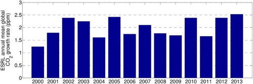
The deterministic spatio-temporal trend of XCO₂ consists of the inherent seasonal CO₂ cycle mainly affected by the biosphere activities (Wunch et al. 2013; Schneising et al. 2014) and an annual CO₂ increase mainly due to the anthropogenic fossil fuel emissions (IPCC 2013). We use the long-term CT2013 data from the year 2000 to 2012 in each 2° latitude band to determine the latitude-dependent seasonal cycle. Following Wunch et al. (2013), we use the ESRL global annual CO₂ growth rate (Figure 4; Conway and Tans 2015) to determine the annual increase of XCO₂ in the trend. As a result, the temporal trend in each latitude band can then be modeled by a simple linear function plus a set of annual harmonic functions (Kyriakidis and Journel 1999; Tsutsumi et al. 2009). The spatial trend within each latitude zone is not considered here. The trend component in Equation (1) can therefore be described as follows:(2)

Figure 4. NOAA Earth System Research Laboratory (ESRL) annual mean global CO₂ growth rate for the year 2000 to 2013, published in ESRL-NOAA webpage: http://www.esrl.noaa.gov/gmd/ccgg/trends/global.html.

where and is the period of 122 time-units, t is the time in time-unit, and ,  and are parameters to be estimated. is the cummulative annual increase for each time-unit determined by the ESRL global annual CO₂ growth rate. i is the order of the harmonic functions, and we use four orders here to specially fit the annual cycle (Wunch et al. 2013), semi-annual oscillation (Jiang et al. 2012), seasonal variation and monthly variation of XCO₂ (Keppel-Aleks, Wennberg, and Schneider 2011). The estimated trend component is then subtracted from the full dataset to yield the spatio-temporal residual component .

3.1.3. Modeling of spatio-temporal correlation structure

In spatio-temporal geostatistical analysis, the optimal kriging prediction of at an unobserved position (s ₀, t₀) can be calculated as the linear weighted sum of the ACOS-GOSAT XCO₂ values that minimizes the mean squared prediction error. The weights for the observations are determined by the geometry of observations and the spatio-temporal covariance or variogram model, which characterizes the spatio-temporal correlation structure of the data. Therefore, estimating and modeling the covariance function or variogram of XCO₂ are crucial steps in kriging prediction for the global land mapping. Due to the non-uniform correlation structure of global XCO₂ variation (Alkhaled et al. 2008), in this study we divide the global land region into 10° bins, producing 11 latitude zones from 40°S to 70°N, and assume that the spatio-temporal correlation structures of the ACOS-GOSAT XCO₂ data within each zone are homogeneous and locally stationary (Haas 1990; Schabenberger and Gotway 2004) for the mapping method. The spatio-temporal empirical variogram (Cressie and Wikle 2011; Zeng et al. 2014) of ACOS-GOSAT XCO₂ data is calculated from the residual component in each 10° latitude zone. The empirical variogram value at the lag is given by(3)

where , and is the cardinality of the set: (s, t) ∈ H such that . (, ) are the spatial tolerance and temporal tolerance. Once the empirical variogram has been constructed, a spatio-temporal variogram model, , is fitted to it. As in Zeng et al. (2014), the spatio-temporal variogram model adopted here is a combination of the product-sum model (De Iaco, Myers, and Posa 2001, 2010) and an extra global nugget model to capture the nugget effect (Cressie 1993; Cressie and Wikle 2011), given by(4)

The following exponential model for the marginal variogram model and is adopted:(5)

where and are the marginal spatial and temporal variograms, [, , , ] = [, , , , , ] are parameters to be estimated, and , , . In the exponential model, is called the range, where the variogram value stabilized at a value, , the partial sill. is called a nugget effect, which is the semi-variance value when spatial and temporal lag are closest to 0. The nugget effect is an important variogram parameter characterizing both the measurement error and the micro-scale variability of the data (Cressie 1993; Chatterjee et al. 2010). A larger nugget effect value typically indicates larger overall variability of microstructure in the data. For each latitude zone, the empirical variogram is calculated from Equation (3) and modeled using the variogram model provided by Equations (4) and (5). To avoid biased result in the edges of the study area, a 5° buffer zone is added in each latitude zone in both the south and north directions. All parameters are estimated simultaneously to overcome the limitation of conventional product-sum fitting (Jost, Heuvelink, and Papritz 2005). The nonlinear, weighted least-square estimation technique (Cressie 1985; Zeng et al. 2014) was used for parameter estimation in this study.

3.1.4. Prediction using space–time kriging with moving cylinder kriging neighborhood

Based on the spatio-temporal variogram model, space–time kriging predicts the value at unobserved location (), from the stochastic residual component }. Suppose that is a prediction of , the kriging method predicts as a linear weighted sum of residual data within a kriging neighborhood (Cressie 1993; De Iaco and Posa 2012) in space and time relative to the prediction location . Assume that the used data number is , then(6)

where is the weight assigned to a known observation so as to minimize the prediction error variance while maintaining unbiasedness of the prediction. The prediction error variance, which is a measurement of prediction uncertainty, is given by(7)

where , , and is the unit vector. To reduce computational complexity and preserve local variability, data used in the prediction were searched within an appropriate spatio-temporal neighborhood centered on the predicting point, called the kriging neighborhood (Cressie 1993; Chiles and Delfiner 2012; De Iaco and Posa 2012). Following the prediction approach in Zeng et al. (2014), the kriging neighborhood used will be a cylinder in space and time as described in Haas (1995). The radii of the initial search range are set to 300 km in space and 20 time-units, the increment lags are 10 km and 1 time-unit for each search process if the number of observations in the cylinder neighborhood is less than 20, and the search range radii limits are set to 500 km and 40 time-units. The position to be predicted will be left as missing data if the available data number within the search range of limit radius is less than 20 points, a threshold value adopted by Watanabe et al. (2015), which has been shown to be an appropriate number for XCO₂ mapping by Zeng et al. (2014). In kriging, extremely high or low data values may have a significant impact on the prediction if there are no other data nearby (Watanabe et al. 2015) in space and time. In this study, we used the bias removal method recommended by Tukey (1977) and Hoaglin, Iglewicz, and Tukey (1986), based on the quartile of the data, to remove the extreme values of the residual component in each latitude zone, before implementing the space–time kriging prediction approach.

3.2. Spatial-only geostatistics for global land mapping

The spatial-only method implemented here for comparison is similar to that for generating monthly GOSAT Level 3 data (Watanabe et al. 2015). The whole XCO₂ dataset is first grouped into monthly datasets (4 years = 48 months), and then the spatial variogram for each month is calculated and modeled by the exponential variogram model (as in Equation (5)). Finally, based on the monthly modeled variograms, spatial-only kriging is applied for mapping global land XCO₂ in each month.

3.3. Cross-validation based on Monte Carlo sampling

Cross-validation is a widely used method for assessing prediction accuracy of statistical models (Arlot 2010), and it can therefore be used to assess the prediction accuracy of the global land mapping approach based on spatio-temporal geostatistics in this study. As above, we use the ACOS-GOSAT XCO₂ dataset . The cross-validation is implemented by first removing a small ratio of observation data and then making its prediction using the remaining dataset. Finally, two datasets, the predicted dataset { and the corresponding original dataset , are obtained. In this study, the following four summary statistics from cross-validation were derived to assess prediction precision using the above two datasets: the correlation coefficient (r² ), the mean absolute prediction error (MAPE), the root mean square error (RMSE) and the percentage of estimation error (PEE) less than 1 ppm. MAPE and RMSE are defined by(8) (9)

A larger r² means a stronger linear association between the predictions and observations. Both MAPE and RMSE measure model accuracy, and conceptually MAPE provides a measurement of average bias for an individual prediction. Smaller values for these two variables indicate better performance. Moreover, the percentage of prediction error (PPE) less than 1 ppm provides a detailed description of the prediction errors. In this study, we carry out a Monte Carlo study by randomly sampling 5% of the data that will be left out in cross-validation, and repeating this process for 100 times. With the ensemble outputs from this Monte Carlo study, we can further assess the uncertainties in these four statistics from cross-validation and uncertainties in parameter estimation for variograms. This study is carried out for both spatial-only and spatial–temporal method, and we further conduct a comparison between them based on all the statistics from cross-validation.

3.4. Implementation workflow

In this study, multi-source datasets and different data processing techniques have been used to generate and evaluate the global land mapping dataset of XCO₂ from satellite observations using spatio-temporal geostatistics. As a conclusion of all the used methodologies, Figure 5 shows a workflow chart for the spatio-temporal mapping process and the evaluation of the mapping data products.

Figure 5. Workflow chart for the spatio-temporal mapping process and the evaluation of the mapping data products in this study. The input datasets are displayed in bold and the numbers in the boxes denote the section numbers in the manuscript.

4. Results and discussions

4.1. Spatio-temporal trend of XCO₂

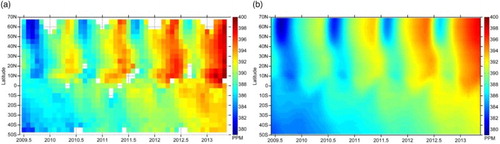
As shown in Equation (1), the spatio-temporal trend of XCO₂ represents the deterministic mean component of the XCO₂ data, and can be obtained by fitting the model in Equation (2) to the CT2013 time series data in each latitude band and then combined to form the spatio-temporal trend component. The parameters in Equation (2) are estimated using CT2013 data from January 2000 to December 2012 and then used to calculate the trend component from June 2009 to May 2013. Figure 6(b) shows the estimated spatio-temporal trend from CT2013 XCO₂ data as a function of latitude and time. As a comparison, Figure 6(a) shows the corresponding spatio-temporal distribution of XCO₂ from original ACOS-GOSAT data aggregated with a grid resolution of 5° in latitude and one month in time. From the figure, we find that the two figures are generally in agreement, indicating that the estimated trend from the CT2013 data well reproduce the spatial and temporal variation of XCO₂ from satellite observations. The results are also consistent with that from Schneising et al. (2014) based on long-term SCIAMACHY XCO₂ data and from WMO (2014) based on ground-based CO₂ observations. Stronger seasonal cycles can be identified in the Northern Hemisphere than in the Southern Hemisphere, indicating a stronger effect of the temporally varying imbalance between photosynthesis and respiration of vegetation in the North Hemisphere (Keppel-Aleks, Wennberg, and Schneider 2011). In the Southern Hemisphere, the seasonal variation is relatively weak. An overall global annual increase can be clearly observed at a rate of about 2 ppm from both the CT2013 trend data and the ACOS-GOSAT data, which is primarily caused by the world-wide consumption of fossil fuels (IPCC 2013).

Figure 6. (a) Overview of the global spatio-temporal distribution of XCO₂ as a function of latitude and time from original ACOS-GOSAT data aggregated with a grid resolution of 5° in latitude and one month in time and (b) the corresponding deterministic spatio-temporal trend calculated from model simulation of CarbonTracker CT2013 XCO₂ data with a grid resolution of 2° in latitude and one time-unit (3-day) in time.

Table 2 summarizes the zonal statistics of all the 10° latitude zones for modeling the spatio-temporal XCO₂ correlation structure, including the zonal central latitudes and the medians and standard deviations of the ACOS-GOSAT data in each latitude zone from June 2009 to May 2013. These description statistics are derived only from ACOS-GOSAT XCO₂ data over land since the ocean glint data are not recommended for science analysis (Nguyen et al. 2014b). It is clear from Table 2 that the standard deviations gradually decrease from north to south, indicating that the ACOS-GOSAT XCO₂ data have larger variability in the north, mainly due to a stronger seasonal cycle than that in the south (Miller et al. 2007). The median values in the Northern Hemisphere are generally larger than those in the Southern Hemisphere. However, in the high latitude of the Northern Hemisphere the median values are underestimated because fewer ACOS-GOSAT XCO₂ retrievals are available in this region during winter when XCO₂ is high. The uncertainties in the estimated variogram parameters are quantified by one standard deviation (), and the uncertainty value of 0.00 in Table 2 means that the uncertainty is actually less than 0.005. From Table 2, we find that most of uncertainties are around 1% and all of them are smaller than 5%, indicating a robust variogram modeling for all the latitudinal zones.

Table 2. Zonal statistics for the 11 bands, including the central latitude of each 10° latitude zone, the number of available data, the median and standard deviation of the ACOS-GOSAT XCO₂ data from June 2009 to May 2013 in the corresponding zone, the parameters of the spatio-temporal variogram model of the ACOS-GOSAT data, and the corresponding nugget/sill ratios in space and time, respectively.

	Zone center latitude	Number of data	Median (ppm)	Standard deviation (ppm)	Estimated parameters for variogram model [, , , , , ]	Spatial ratio nugget/sill	Temporal ratio nugget/sill
Zone 1	65°N	10,462	387.76	4.73	[1.84 ± 0.02, 170.73 ± 4.15, 3.82 ± 0.04, 13.08 ± 0.22, 0.26 ± 0.00, 1.22 ± 0.02]	0.40 ± 0.01	0.24 ± 0.00
Zone 2	55°N	16,461	389.02	4.59	[1.43 ± 0.01, 238.22 ± 3.49, 2.44 ± 0.02, 14.70 ± 0.14, 0.27 ± 0.00, 1.28 ± 0.01]	0.47 ± 0.00	0.34 ± 0.00
Zone 3	45°N	49,821	389.88	4.20	[1.35 ± 0.01, 319.44 ± 4.91, 1.84 ± 0.01, 13.26 ± 0.13, 0.34 ± 0.00, 1.30 ± 0.01]	0.49 ± 0.00	0.41 ± 0.00
Zone 4	35°N	44,095	390.65	3.82	[1.31 ± 0.01, 261.64 ± 6.97, 2.04 ± 0.01, 16.31 ± 0.19, 0.41 ± 0.00, 1.21 ± 0.01]	0.48 ± 0.00	0.37 ± 0.00
Zone 5	25°N	18,374	391.23	3.58	[1.13 ± 0.01, 167.18 ± 4.65, 3.16 ± 0.05, 42.15 ± 0.92, 0.32 ± 0.00, 1.03 ± 0.01]	0.48 ± 0.00	0.25 ± 0.00
Zone 6	15°N	8571	391.82	3.68	[1.44 ± 0.01, 172.63 ± 4.04, 2.75 ± 0.14, 20.82 ± 1.53, 0.32 ± 0.00, 0.87 ± 0.01]	0.38 ± 0.00	0.24 ± 0.01
Zone 7	5°N	2774	391.81	3.57	[2.38 ± 0.07, 384.00 ± 19.16, 2.36 ± 0.21, 17.02 ± 2.31, 0.38 ± 0.01, 0.62 ± 0.02]	0.21 ± 0.01	0.21 ± 0.01
Zone 8	5°S	6678	390.22	2.67	[1.24 ± 0.01, 397.80 ± 5.41, 1.37 ± 0.04, 23.60 ± 0.97, 0.63 ± 0.00, 0.74 ± 0.00]	0.37 ± 0.00	0.35 ± 0.01
Zone 9	15°S	31,771	389.77	2.69	[0.91 ± 0.00, 235.32 ± 2.58, 1.14 ± 0.02, 15.57 ± 0.46, 0.79 ± 0.00, 0.70 ± 0.00]	0.43 ± 0.00	0.38 ± 0.00
Zone 10	25°S	44,436	389.38	2.73	[0.90 ± 0.00, 184.73 ± 1.74, 1.21 ± 0.03, 17.04 ± 0.56, 0.78 ± 0.00, 0.66 ± 0.00]	0.43 ± 0.00	0.35 ± 0.00
Zone 11	35°S	20,754	389.05	2.78	[0.98 ± 0.01, 129.41 ± 2.17, 1.34 ± 0.02, 18.35 ± 0.53, 0.69 ± 0.00, 0.58 ± 0.01]	0.37 ± 0.00	0.30 ± 0.00

Notes: Uncertainties of the variogram-related parameters, quantified by one standard deviation, are derived from the Monte Carlo study described in Section 3.3.

4.2. Spatio-temporal empirical variogram and variogram modeling

Figure 7 shows the spatio-temporal empirical variograms calculated from the full ACOS-GOSAT dataset for the 11 latitude zones, and the corresponding spatio-temporal variogram models fitted by the product-sum model as described in Equations (4) and (5). The statistics for the 11 latitude zones are given in Table 2. As shown in Cambardella et al. (1994) and Fu et al. (2014), the ratio of nugget to sill, expressed as percentage, can be used as an indicator to classify data dependence. In general, a ratio of less than 25% indicates a strong spatial or temporal dependence, between 25% and 75% indicates a moderate spatial or temporal dependence and larger than 75% indicates a weak spatial or temporal dependence. The ratios of nugget to sill of both space and time for the 11 latitude zones are listed in Table 2. All the ratio values are less than 0.5 indicating that all the zonal XCO₂ data show either moderate or strong spatial and temporal dependences. Moreover, the temporal ratio values are all lower than the spatial ratio values in the same latitude zone, showing stronger dependences in time between XCO₂ data than in space, justifying the use of spatio-temporal geostatistics in this study, which makes full use of the joint spatial and temporal dependencies between observations.

Figure 7. For each latitude zone, the left plot shows the spatio-temporal empirical variogram of the ACOS-GOSAT XCO₂ residual data after the spatio-temporal trend is excluded, and the right plot shows its fitted variogram model using the product-sum model in Equation (4).

From the estimated parameters for spatio-temporal variogram models shown in Table 2 and the experimental variograms and the corresponding fitted models in Figure 7, we find that the spatial and temporal marginal variogram models shown in Equation (5) vary considerably between latitude zones, and all the joint spatio-temporal variograms present different shapes, indicating differences of spatio-temporal correlation structure for different latitude zones. These differences illustrate the spatial heterogeneity of the observed space–time correlation structure in global ACOS-GOSAT XCO₂ data. From Table 2, furthermore, we find that the nugget effects, a measure of both the measurement error and micro-scale variability of the XCO₂ data, in the Northern Hemisphere are generally greater than that in the Southern Hemisphere, which indicates greater overall data variability in the Northern Hemisphere.

4.3. Cross-validation and comparison with spatial-only method

Results from cross-validation based on Monte Carlo sampling are shown in Table 3. For our developed spatio-temporal method, the r² is 0.94 ± 0.00, indicating a very strong correlation between the original ACOS-GOSAT data and the predictions. Moreover, the MAPE is 0.93 ± 0.01 ppm, indicating that the averaged absolute error of each prediction is less than 1 ppm. From the prediction errors, we find that more than 65.53 ± 0.42% of the prediction errors are less than 1 ppm. These summary statistics from cross-validation for the global land with four years of ACOS-GOSAT data are better than those found for China as a study region with only two years of ACOS-GOSAT data by Zeng et al. (2014). The improvement may be due to the facts that in this study more satellite data are available, and the zonal characteristics of XCO₂ are fully considered, while Zeng et al. (2014) simply assumed a uniform spatio-temporal trend. All the statistics from this cross-validation study indicate that the global land mapping method based on spatio-temporal geostatistics is effective, and we can therefore generate precise maps of XCO₂ using this method from the full dataset of ACOS-GOSAT observations.

Table 3. Summary statistics for the developed spatio-temporal method and spatial-only method from global land cross-validation based on the Monte Carlo sampling technique, including correlation coefficient (r²), MAPE, RMSE, and percentage of prediction error within 1 ppm (PPE1) for the global mapping approach.

r^2	MAPE (ppm)	RMSE (ppm)	PPE1 (%)
Spatio-temporal method
0.94 ± 0.00	0.93 ± 0.01	1.28 ± 0.01	65.53 ± 0.42
Spatial-only method
0.92 ± 0.00	1.06 ± 0.01	1.41 ± 0.01	58.62 ± 0.43

Note: Both mean and one standard deviation of the ensemble outputs from cross-validation are shown.

Moreover, we compare prediction precision between the spatio-temporal and spatial-only methods in terms of cross-validation statistics. For the spatial-only method, the four statistics are shown in Table 3, and these statistics indicate less precision and larger prediction error for the spatial-only method than the spatio-temporal method. Therefore, these statistics justify the improvement of the developed spatio-temporal method over the traditional spatial-only method in terms of cross-validation.

4.4. Comparison with the total carbon column observing network (TCCON)

TCCON provides an essential data source for validating satellite XCO₂ retrievals and the data have been widely used for validation of satellite XCO₂ retrievals using different retrieval algorithms in several previous studies (e.g. Butz et al. 2011; Morino et al. 2011; Wunch et al. 2011a; Cogan et al. 2012; Dils et al. 2014; Nguyen et al. 2014b). In this study, we perform comparison between TCCON XCO₂ data and the XCO₂ time series reconstructed using the developed global land mapping approach from ACOS-GOSAT XCO₂ observations. As suggested by Rodgers and Connor (2003), when comparing two observations from different instruments, the retrievals should be calculated using a common a-priori profile, and the smoothing effect of the retrievals should be considered by applying the averaging kernels. A detailed description of the use of the averaging kernel for comparing ACOS-GOSAT and TCCON data can be found in Wunch et al. (2011a) and Nguyen et al. (2014b). Following the instructions in Section 2.1 of Nguyen et al. (2014b), we apply the ACOS-GOSAT averaging kernel equation to TCCON data from the 16 chosen sites to obtain what ACOS-GOSAT would have retrieved at the TCCON sites assuming the TCCON profile as ‘truth’. The TCCON data are chosen using coincidence criteria of within ±2 hours of GOSAT overpass time, which is about 13:00 local time for most sites, and 3-day (one time-unit) median is calculated for the comparison if the observation number within the time-unit is at least 3. Since the XCO₂ estimates at each TCCON site are obtained from a kriging neighborhood within 500 km in space, as described in Section 3.1, the original ACOS-GOSAT XCO₂ data within 500 km of each TCCON site will be chosen, and similarly, the 3-day median will be calculated for comparison. As a result, Figure 8 shows the comparison of the XCO₂ estimates from this study, the coincident TCCON XCO₂ 3-day median data, and the coincident ACOS-GOSAT XCO₂ observations and their 3-day medians.

Figure 8. Temporal variation comparison for the 16 TCCON sites. As shown in these panels, the original ACOS-GOSAT XCO₂ retrievals within 500 km of the TCCON site are in gray dots, the corresponding medians are in black dots when at least three data points are available within the time-unit. The TCCON data, smoothed by applying the ACOS-GOSAT averaging kernel, are indicated by blue circles. The data are chosen using coincidence criteria of within ±2 hours of GOSAT overpass time, and a 3-day (one time-unit) median is calculated for the comparison if the number of data points within the time-unit is at least 3. The predicted TCCON site XCO₂ time series using the global land mapping approach are indicated by the red line.

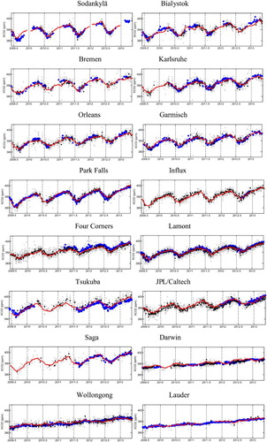
As the global land mapping method is a data-driven prediction approach, the resulting predictions will rely heavily on the original data. From Figure 8, it can be observed that the predictions go through the original satellite observations and agree well with the median data. Table 4 gives a more detailed summary statistics in terms of the number of coincident data pairs, averaged bias, averaged absolute bias and standard deviation of the bias between the mapping dataset and TCCON (hereafter referred to as Mapping-TCCON), as well as between ACOS-GOSAT 3-day median and TCCON (hereafter referred to as ACOS-TCCON). From Table 4, we find that the numbers of coincident data pairs for Mapping-TCCON range from 32 at Influx to 416 at Lamont, while the numbers for all sites are smaller for ACOS-TCCON which is based on the 500-km geographical coincident criteria. The difference of numbers of coincident data pairs can be obviously seen in Figure 9, which shows plots of the statistics in Table 4. For Mapping-TCCON, the averaged biases, except Four Corners (1.62 ppm), are within 1 ppm, and standard deviations for all the sites are close, ranging from 0.66 to 1.58 ppm. In terms of averaged absolute biases, Mapping-TCCON are smaller than ACOS-TCCON for 13 out of 16 stations. Overall, the XCO₂ predictions at all TCCON sites are in good agreement with the TCCON data, with an overall averaged bias of 0.01 ppm, an overall averaged absolute bias of 0.94 ppm and a standard deviation of 1.22 ppm. For ACOS-TCCON, the overall averaged bias is −0.35 ppm and the corresponding standard deviation is 1.38 ppm, which is consistent with the result from the ACOS-GOSAT XCO₂ data after filtering and bias correction as described in ACOS Data User's Guide (13). Unfortunately, both TCCON and ACOS-GOSAT observation are affected by clouds, so when few ACOS-GOSAT data are available, few TCCON retrievals are available either. However, with all possible plots and statistics given, we believe that Figure 8 and Table 4 have provided a robust assessment of the mapping dataset compared to TCCON.

Figure 9. Statistics of comparison between the geostatistical mapping results and the TCCON data (smoothed by applying the ACOS-GOSAT averaging kernel), and between the ACOS-GOSAT 3-day median XCO₂ data and TCCON data, hereafter referred to as Mapping-TCCON and ACOS-TCCON, respectively. The statistics are also shown in Table 4. The top panel shows the comparison of XCO₂ biases between Mapping-TCCON and ACOS-TCCON, while the down panel shows the comparison of numbers of coincident data pairs between them.

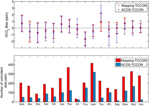
Table 4. Statistics of comparison between the geostatistical mapping results and the TCCON data (smoothed by applying the ACOS-GOSAT averaging kernel), and between the ACOS-GOSAT 3-day median XCO₂ data and TCCON data, hereafter referred to as Mapping-TCCON and ACOS-TCCON, respectively.

		Mapping-TCCON				ACOS-TCCON
Sites	Location [longitude, latitude]	Coincident data pairs	Averaged biases (ppm)	Averaged absolute bias (ppm)	Standard deviation (ppm)	Coincident data pairs	Averaged biases (ppm)	Averaged absolute bias (ppm)	Standard deviation (ppm)
Sodankylä	[26.63, 67.37]	204	0.72	1.05	1.22	50	0.62	1.18	1.22
Bialystok	[23.03, 53.23]	171	−0.56	1.30	1.58	47	−0.47	0.77	0.96
Bremen	[8.85, 53.10]	86	−0.72	1.28	1.51	38	−0.76	1.17	1.43
Karlsruhe	[8.44, 49.10]	190	−0.30	0.97	1.17	86	−0.52	1.09	1.42
Orleans	[2.11, 47.97]	150	−0.47	0.97	1.10	56	−0.72	1.28	1.45
Garmisch	[11.06, 47.48]	253	0.57	1.02	1.14	100	0.56	1.09	1.26
Park Falls	[−90.27, 45.94]	371	0.22	0.78	0.97	123	0.30	0.82	1.05
Influx	[−86.00, 39.86]	32	−0.26	0.63	0.76	23	−0.04	1.02	1.42
FourCorners	[−108.48, 36.80]	206	−1.62	1.68	1.05	151	−1.72	1.72	1.00
Lamont	[−97.49, 36.60]	416	−0.41	0.79	0.90	320	−0.60	0.91	1.00
Tsukuba	[140.12, 36.05]	225	0.86	1.29	1.37	43	2.24	2.24	1.24
JPL/Caltech	[−118.18, 34.20]	148	−0.21	0.90	1.11	99	−1.19	1.58	1.44
Saga	[130.29, 33.24]	135	−0.01	0.67	0.83	12	−0.86	1.21	1.39
Darwin	[130.89, −12.43]	270	0.69	0.91	0.84	118	−0.10	0.66	0.85
Wollongong	[150.88, −34.41]	327	0.14	0.76	0.91	167	−0.00	0.88	1.11
Lauder	[169.68, −45.05]	281	−0.01	0.53	0.66	23	0.16	0.71	0.92
Overall		3465	−0.01	0.94	1.22	1456	−0.35	1.10	1.38

Notes: The statistics include the location information, and statisics of the differences computed by subtracting the TCCON median XCO₂ from the mapping predictions and ACOS-GOSAT XCO₂ 3-day medians, respectively, at the corresponding TCCON sites.

From Figure 9, the averaged biases of Mapping-TCCON for most sites are generally closer to zeros than ACOS-TCCON, with overall averaged bias of 0.01 ppm for Mapping-TCCON and −0.35 ppm for ACOS-TCCON. It indicates that the mapping dataset is more accurate than ACOS-GOSAT median data when compared to TCCON. However, the standard deviations of the bias are almost the same between Mapping-TCCON and ACOS-TCCON, with an overall standard deviation of 1.22 and 1.38 ppm, respectively. Moreover, the dependence of the developed mapping method on the original satellite data can be clearly observed in Figure 9, where the averaged bias of Mapping-TCCON is positively correlated to that of ACOS-TCCON, indicating that the prediction precision of the global land mapping will increase as XCO₂ retrieval precision of ACOS-GOSAT improves.

Furthermore, the global land mapping method developed in this study also provides an effective spatio-temporal geostatistical method for collocating satellite XCO₂ data with the ground observations, as investigated in Nguyen et al. (2014b). More ground observations should be used to validate this mapping dataset as more and more TCCON sites are available in the future, particularly for the vast region in Africa and Asia where TCCON data are still unavailable. At the same time, the quality of TCCON retrievals is also improving and therefore provides more accurate data for validation of the satellite retrievals. For example, as noted in the data description in the TCCON website (https://tccon-wiki.caltech.edu/), all Four Corners TCCON GGG2012 version XCO₂ retrievals are high biased by ∼0.28% or ∼1.1 ppm due to an error in the surface pressure used in the retrievals. The error will be fixed in the new version and this will lead to a ∼1.1 ppm offset from the absolute bias (1.68 ppm) compared with satellite data as shown in Table 4.

4.5. Assessment of mapping results

4.5.1. Generated mapping dataset

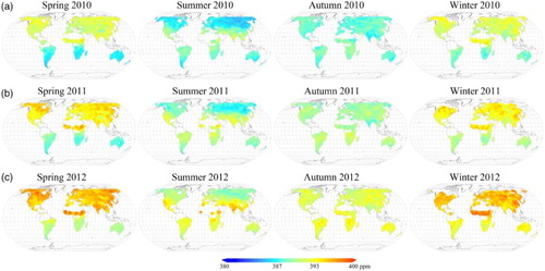
Examples of spatial distribution of the mapping XCO₂ data from 2010 to 2012 are shown in Figure 10 by taking their seasonal mean values. In summer, globally, a relatively lower XCO₂ value can be observed in the high latitude region of the Northern Hemisphere than that in the low latitude region, mainly due to the large CO₂ uptake by the growing forest in North Hemisphere. In other seasons, the XCO₂ value is higher in the Northern Hemisphere than that in the Southern Hemisphere. The geostatistical mapping data show wider coverage and more detailed spatial distributions of XCO₂, especially in some key regions, such as south China and Central Asia, than the original satellite retrievals with sparse coverage as shown in Figure 1.

Figure 10. Spatial distribution of seasonal mean XCO₂ from global land mapping for three years of 2010 in panel (a), 2011 in panel (b) and 2012 in panel (c). Four images in each panel corresponds to spring, summer, autumn and winter from left to right, respectively. These global land mapping seasonally averaged results in 1° by 1° grid are obtained by calculating the seasonal mean from the geostatistical mapping results when at least one data is available for each of the three months in that season. As usual, the season spring includes three months of March, April and May, summer includes June, July and August, autumn includes September, October and November, and winter includes December, next year January and February.

4.5.2. Prediction uncertainty

For each geostatistical prediction, the corresponding kriging variance, defined in Equation (7), can be obtained at the same time as a measure of prediction uncertainty. Kriging variance is calculated without the knowledge of the true XCO₂ distribution, and it is determined by both the density of ACOS-GOSAT XCO₂ observations and the data variability in the neighborhood of the prediction location. Generally speaking, areas with more homogeneous XCO₂ variation and denser observations surrounding the prediction location will have lower prediction uncertainty (Chiles and Delfiner 2012; Hammerling, Michalak, and Kawa 2012). Figure 11 shows the spatial and temporal variations of the prediction uncertainty from the global land mapping. The prediction uncertainty is unevenly distributed in space, which is generally in negative correlation with the spatial distribution of observation number density as shown in Figure 2(a). Predictions in the Southern Hemisphere, where a large number of observations are available with lower variability, present a relatively smaller uncertainty, which can clearly be seen in Figure 11(b). However, regions with fewer observations and larger variability present a larger prediction uncertainty, as in the high latitude Northern Hemisphere. Temporally, the time series of spatial averaged prediction uncertainty varies from 1.0 to 2.6 ppm and we find them negatively correlated with a time series of available ACOS-GOSAT XCO₂ data number in all latitudinal zones (not shown).

Figure 11. Kriging standard deviations of prediction, a measurement of prediction uncertainty. (a) Spatial distribution, which is obtained by averaging the kriging standard deviations over all time-units in the global land. (b) Temporal distribution for the 11 zones, which are averaged for each time-unit of each zone from June 2009 to May 2013. For each time-unit and each zone, the averages are calculated only when more than 50% of the data are available.

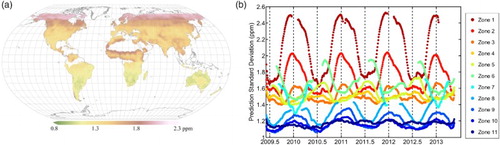
To assess how well the prediction uncertainties describe the prediction errors, we use the ensemble outputs from cross-validation based on the Monte Carlo sampling technique, and calculate the coverage PPEs by the prediction uncertainties for our developed spatio-temporal method. This coverage percentage is 70.35 ± 0.39%, which indicates that more than 70% of the prediction errors can be constrained by the prediction uncertainty map shown in Figure 11. For the spatial-only method, it is 69.04 ± 0.42%, which is slightly smaller but not significantly different from that of the spatio-temporal method.

4.6. Comparison with model simulations of XCO₂

We compare the original ACOS-GOSAT XCO₂ data, the global land mapping XCO₂ dataset, and the model simulations of XCO₂ from CT2013 and GEOS-Chem by illustrating and analyzing their spatio-temporal variation as a function of latitude and time. The XCO₂ value for each specific latitude bin and time bin is obtained by calculating the zonal mean of XCO₂ within the time lag. Figure 12(a) shows the result for the global land mapping data, with latitude bins of 1° and temporal bins of 3 days. The zonal mean data in Figure 12(a) in the subtropical region are excluded when the available data number within the zonal band are less than 15, which is the number of pixels of equatorial Africa, to avoid bias in calculation especially around the equatorial region where few mapping data are available. Figure 12(b) shows the result from original ACOS-GOSAT XCO₂ observations, with latitude bins of 5° and temporal bins of one month, which is the same with Figure 6(a). Figure 12(c) and (d) is the results for CT2013 from June 2009 to December 2012 and GEOS-Chem for 2010, respectively. Strong seasonal XCO₂ variations in northern high and mid-latitudes can be observed from these panels, but in the Southern Hemisphere they are indistinct. In addition, the steady annual increase of global XCO₂ mainly due to the burning of fossil fuels can be easily identified in both the Northern and Southern Hemisphere.

Figure 12. Overview of the global spatio-temporal distribution of XCO₂ as a function of latitude and time, from (a) global land mapping dataset with a grid resolution of 1° in latitude and one time-unit in time, (b) original ACOS-GOSAT data with a grid resolution of 5° in latitude and one month in time, and model simulations from both (c) CarbonTracker CT2013 data with a grid resolution of 2° in latitude and one time-unit in time and (d) GEOS-Chem data in 2010 with a grid resolution of 4° in latitude and one time-unit in time, and an overview of the differences of global spatio-temporal distribution of XCO₂ between (e) global land mapping dataset and CarbonTracker2013 data, (f) global land mapping dataset and GEOS-Chem data, (g) original ACOS-GOSAT data and CarbonTracker CT2013 data, and (h) original ACOS-GOSAT data and GEOS-Chem data.

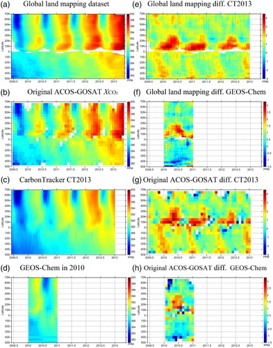
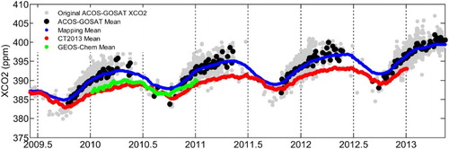
Figure 12(e) and (f) shows the differences by subtracting CT2013 in Figure 12(c) and GEOS-Chem in Figure 12(d), respectively, from the mapping dataset in Figure 12(a). For most regions, the differences are generally within 2 ppm, indicating that the spatio-temporal variation of the mapping dataset and the model simulations are in agreement for most of the region. However, large difference of 3–4 ppm can be identified in the region of 5–15°N during late winter (January and February) and early spring (March) each year. This latitude zone mainly covers the central African tropical region. A similar result can also be concluded from Figure 12(g) and (h), which shows the difference by subtracting the result of both models from the original ACOS-GOSAT dataset in Figure 12(b). In Figure 13, we specifically analyze the data in this central African land region within 5–15° N in latitude and 20°W to 40°E in longitude as specified in Figure 2(a), by comparing the time series of the original satellite observations, mapping dataset, CT2013 data and the GEOS-Chem data. As expected, the predictions are consistent with the original satellite observations and their mean values, indicating that the data-driven feature of the geostatistical prediction method although the trend component is derived from the CT2013 model simulation data. Moreover, the satellite data and model simulations generally agree during summer time, while larger difference can be observed from January to March, which is consistent with the conclusions from Figure 12. This difference may be due to the deficiency of CarbonTracker in constraining tropical biomass burning CO₂ fluxes because of the lack of atmospheric observations due to the sparse observational network in this region (Peters et al. 2007). Moreover, the thin clouds that often occur in the tropics may have an impact on the retrievals of satellite CO₂ and contribute to the XCO₂ difference in the tropical region, as described in the study comparing XCO₂ data from SCIAMACHY and CarbonTracker by Heymann et al. (2012).

Figure 13. The panel shows the XCO₂ time series in central Africa within 5°N to 15°N in latitude and 20°W to 40°E in longitude. The original ACOS-GOSAT data indicated by gray dots and its mean in black dots calculated when at least three data points are available within the time-unit. The mapping dataset mean is indicated by the blue line, CarbonTracker CT2013 data mean by the red line and GEOS-Chem data mean by the green line.

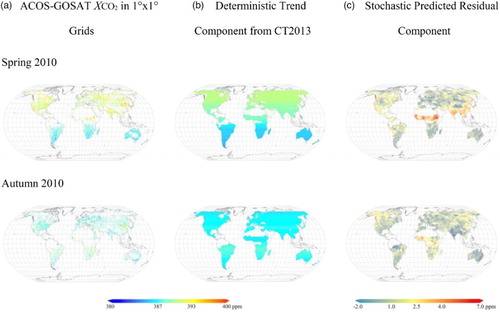
From Figure 13, we can see that there is a big difference in the amplitude of seasonal cycle between CT2013 data and the mapping data even though the temporal trend in the geostatistical prediction is derived from CT2013. To understand more on the trend data, Figure 14 shows the decomposition of the mapping data into trend component and residual component for two seasons of Spring 2010 and Autumn 2010, when the differences are the largest and smallest, respectively. We can see that the trend component (panel (b)) generally represents the global meridian trend of the original data (panel (a)), and the predicted residual component, on the other hand, well presents the local variation of XCO₂. In Spring 2010, large residual value can be seen in central Africa and southern and eastern Asia because the trend components are not well capturing the small-scale variations in these two regions where strong natural emission and anthropogenic emission dominate, respectively. While in Autumn 2010, the residuals are small, indicating consistency between the model simulation and satellite observations, which can also be seen from Figure 13. Figure 14 indicates that the contribution of predicted residual component depends on the performance of the trend component. If the trend component do not performs well, then the residual component contribution will be large so that the final prediction results will always be consistent with the observations.

Figure 14. (a) Original ACOS-GOSAT XCO₂ distributions averaged over 1°×1° grids, and the corresponding mapping decompositions, including (b) averaged deterministic trend component from CT2013 and (c) averaged stochastic residual component for Spring 2010 and Autumn 2010, respectively.

5. Conclusions

Global geostatistical mapping of satellite-observed XCO₂ data is a useful gap-filling method for dealing with satellite data that are sparse and irregularly distributed in space and time. In this study, we have demonstrated a valid method based on spatio-temporal geostatistics for global land mapping of satellite XCO₂ observations from ACOS-GOSAT. We find that the method presents a significant high correlation coefficient of 0.94 between the predictions and observations in cross-validation, and moreover, the mapping results are in good agreement with the data from TCCON sites with overall bias of less than 0.01 ppm and standard deviation of the difference of 1.22 ppm, which show the effectiveness of the global land mapping method developed in this study. Furthermore, we demonstrate the difference and similarity between the geostatistical mapping of satellite data and model simulations of XCO₂ data from CarbonTracker2013 and GEOS-Chem by analyzing their spatio-temporal distribution. From the comparison, we find that the model outputs and the satellite data show consistent spatial patterns in most regions, except in tropical central Africa where there is a large discrepancy during late winter and early spring. This discrepancy may result from two possible causes related to model simulations and satellite retrievals. First, the lack of atmospheric observations in this region leads to the deficiency of CarbonTracker in constraining tropical biomass burning CO₂ fluxes (Peters et al. 2007). Second, the retrievals of XCO₂ in this region may be affected by thin clouds that often occur in the tropics (Heymann et al. 2012). Further investigation and validation are needed to explain the underlying causes of this discrepancy. We can see that the relatively high spatio-temporal resolution of the global land mapping dataset enables us to identify the locations and times of the discrepancies between the satellite retrievals and model simulations. Such detailed comparisons can provide potential evidences for further improvement of both satellite data and model data. Moreover, in this study, the spatio-temporal geostatistical prediction method has been used to reconstruct the time series of XCO₂ at TCCON sites, making it an effective method for collocating satellite XCO₂ data with ground-based data (e.g. Nguyen et al. 2014b).

The generated global land mapping XCO₂ data in this study, with continuous data distribution in space and time, well present the spatio-temporal variations of XCO₂ that are hard to directly infer from the sparse coverage of original satellite data retrievals. Therefore, it provides a new global geospatial dataset in global understanding of greenhouse gases dynamics and global warming. Specifically, the mapping dataset will play potential roles in evaluating the modeled CO₂ fields from carbon flux estimates coupled with an atmospheric transport model, as discussed in Hammerling et al. (2012), detection of atmospheric CO₂ enhancement due to anthropogenic emissions, as discussed in Keppel-Aleks et al. (2013) and assessment of biospheric activities in the global scale, as discussed in Schneising et al. (2014). Recently, Liu et al. (2015) has shown a promising application of the mapping data in viewing the spatial patterns of CO₂ sources and sinks.

Some gaps still exist in the mapping dataset, because (1) there are areas where no observations are available, such as the Sahara desert area where data observed in median-gain mode were filtered before further analysis and (2) we limit the kriging neighborhood to a spatial range of 500 km in order to make predictions efficiently using the most related surrounding dataset to the predictors. As a potential solution, the strength of the model data may be further incorporated in a data assimilation way to map some areas where data are extremely sparse (e.g. van de Kassteele et al. 2009; Chatterjee et al. 2010) since the model can well reproduce the large-scale features of atmospheric CO₂. Furthermore, the global land mapping method developed in this study depends on the assumption of uniform spatio-temporal correlation structures in the same latitudinal zone. As more satellite XCO₂ data become available in the future, we will be able to investigate the characteristics of correlation structures within each zone over different time interval, such as every season. Moreover, in comparison between spatio-temporal and spatial-only approach using cross-validation, leaving out larger regions would conceivably better highlight the advantage of a spatio-temporal approach where temporal correlation can provide large benefits given the lack of nearby data. This will also be our future work.

Acknowledgements

We acknowledge John Robinson from National Institute of Water and Atmospheric Research in New Zealand for providing the Lauder TCCON data, and Laura T. Iraci from NASA Ames Research Center for providing the Influx TCCON data. The ACOS-GOSAT v3.3 data were produced by the ACOS/OCO-2 project at the Jet Propulsion Laboratory, California Institute of Technology, and obtained from the ACOS/OCO-2 data archive maintained at the NASA Goddard Earth Science Data and Information Services Center. We also acknowledge the GOSAT Project for acquiring the spectra. CarbonTracker CT2013 results are provided by NOAA ESRL, Boulder, Colorado, USA from the website at http://carbontracker.noaa.gov. The GEOS-Chem model (http://www.geos-chem.org/) is managed by the GEOS-Chem Support Team, based at Harvard University and Dalhousie University with support from the US NASA Earth Science Division and the Canadian National and Engineering Research Council.

Disclosure statement

No potential conflict of interest was reported by the authors.

ORCID

Zhao-Cheng Zeng http://orcid.org/0000-0002-0008-6508

References

- ACOS Data User's Guide. 2014. “ACOS Level 2 Standard Product Data User's Guide, v3.3, Goddard Earth Sciences Data and Information Services Center.” Accessed June 2014. http://disc.sci.gsfc.nasa.gov/acdisc/documentation/ACOS_v3.3_DataUsersGuide.pdf.
- Alkhaled, A., Anna M. Michalak, Kawa S. Randolph, Seth C. Olsen, and Wang Jih-Wang. 2008. “A Global Evaluation of the Regional Spatial Variability of Column Integrated CO2 Distributions.” Journal of Geophysical Research 113: 1–17. doi: 10.1029/2007JD009693
- Arlot, S. 2010. “A Survey of Cross-Validation Procedures for Model Selection.” Statistics Surveys 4: 40–79. doi: 10.1214/09-SS054
- Boesch, H., D. Baker, B. Connor, D. Crisp, and C. Miller. 2011. “Global Characterization of CO2 Column Retrievals From Shortwave-Infrared Satellite Observations of the Orbiting Carbon Observatory-2 Mission.” Remote Sensing 3: 270–304. doi: 10.3390/rs3020270
- Bovensmann, H., M. Buchwitz, J. P. Burrows, M. Reuter, T. Krings, K. Gerilowski, O. Schneising, J. Heymann, A. Tretner, and J. Erzinger. 2010. “A Remote Sensing Technique for Global Monitoring of Power Plant CO2 Emissions From Space and Related Applications.” Atmospheric Measurement Techniques 3: 781–811. doi: 10.5194/amt-3-781-2010
- Bovensmann, H., J. P. Burrows, M. Buchwitz, J. Frerick, S. Noël, V. V. Rozanov, K. V. Chance, and A. P. H. Goede. 1999. “SCIAMACHY-Mission Objectives and Measurement Modes.” Journal of the Atmospheric Sciences 56: 127–150. doi: 10.1175/1520-0469(1999)056<0127:SMOAMM>2.0.CO;2
- Buchwitz, M., R. de Beek, J. P. Burrows, H. Bovensmann, T. Warneke, J. Notholt, J. F. Meirink, et al. 2005. “Atmospheric Methane and Carbon Dioxide from SCIAMACHY Satellite Data: Initial Comparison with Chemistry and Transport Models.” Atmospheric Chemistry and Physics 5: 941–962. doi: 10.5194/acp-5-941-2005
- Buchwitz, M., M. Reuter, O. Schneising, H. Boesch, S. Guerlet, B. Dils, I. Aben, et al. 2013. “The Greenhouse Gas Climate Change Initiative (GHG-CCI): Comparison and Quality Assessment of Near-Surface-Sensitive Satellite-Derived CO2 and CH4 Global Data Sets.” Remote Sensing of Environment 162: 344–362. doi: 10.1016/j.rse.2013.04.024
- Butz, A., S. Guerlet, O. Hasekamp, D. Schepers, A. Galli, I. Aben, C. Frankenberg, et al. 2011. “Toward Accurate CO2 and CH4 Observations from GOSAT.” Geophysical Research Letters 38: 1–6. doi: 10.1029/2011GL047888
- Cambardella, C. A., T. B. Moorman, T. B. Parkin, D. L. Karlen, J. M. Novak, R. F. Turco, and A. E. Konopka. 1994. “Field-scale Variability of Soil Properties in Central Iowa Soils.” Soil Science Society of America Journal 58: 1501–1511. doi: 10.2136/sssaj1994.03615995005800050033x
- Chatterjee, A., Anna M. Michalak, Ralph A. Kahn, Susan R. Paradise, Amy J. Braverman, and Charles E. Miller. 2010. “A Geostatistical Data Fusion Technique for Merging Remote Sensing and Ground-Based Observations of Aerosol Optical Thickness.” Journal of Geophysical Research 115: 1–12. doi: 10.1029/2009JD013765
- Chiles, J. P., and P. Delfiner. 2012. Geostatistics: Modeling Spatial Uncertainty. 2nd ed. New York, NY: Wiley.
- Ciais, P., A. J. Dolman, A. Bombelli, R. Duren, A. Peregon, P. J. Rayner, C. Miller, et al. 2014. “Current Systematic Carbon-Cycle Observations and the Need for Implementing a Policy-Relevant Carbon Observing System.” Biogeosciences 11: 3547–3602. doi: 10.5194/bg-11-3547-2014
- Cogan, A. J., H. Boesch, R. J. Parker, L. Feng, P. I. Palmer, J.-F. L. Blavier, N. M. Deutscher, et al. 2012. “Atmospheric Carbon Dioxide Retrieved from the Greenhouse Gases Observing SATellite (GOSAT): Comparison with Ground-Based TCCON Observations and GEOS-Chem Model Calculations.” Journal of Geophysical Research: Atmospheres 117: 1–17. doi: 10.1029/2012JD018087
- Connor, B. J., Hartmut Boesch, Geoffrey Toon, Bhaswar Sen, Charles Miller, and David Crisp. 2008. “Orbiting Carbon Observatory: Inverse Method and Prospective Error Analysis.” Journal of Geophysical Research: Atmospheres 113: 1–14. doi: 10.1029/2006JD008336
- Conway, T., and P. Tans. 2015. “Annual Mean Global Carbon Dioxide Growth Rates.” Accessed 15 February 2015. http://www.esrl.noaa.gov/gmd/ccgg/trends/global.html. NOAA/ESRL.
- Cressie, N. 1985. “Fitting Variogram Models by Weighted Least Squares.” Journal of the International Association for Mathematical Geology 17: 563–586. doi: 10.1007/BF01032109
- Cressie, N. 1993. Statistics for Spatial Data. New York: Wiley.
- Cressie, N., and C. K. Wikle. 2011. Statistics for Spatiotemporal Data. New York: Wiley.
- Crisp, D., R. M. Atlas, F.-M. Breon, L. R. Brown, J. P. Burrows, P. Ciais, B. J. Connor, et al. 2004. “The Orbiting Carbon Observatory (OCO) Mission.” Advances in Space Research 34: 700–709. doi: 10.1016/j.asr.2003.08.062
- Crisp, D., B. M. Fisher, C. O'Dell, C. Frankenberg, R. Basilio, H. Bösch, L. R. Brown, et al. 2012. “The ACOS CO2 Retrieval Algorithm – Part II: Global XCO2 Data Characterization.” Atmospheric Measurement Techniques 5: 687–707. doi: 10.5194/amt-5-687-2012
- De Iaco, S. 2010. “Space–Time Correlation Analysis: A Comparative Study.” Journal of Applied Statistics 37: 1027–1041. doi: 10.1080/02664760903019422
- De Iaco, S., D. E. Myers, and D. Posa. 2001. “Space–Time Analysis Using a General Product–sum Model.” Statistics & Probability Letters 52: 21–28. doi: 10.1016/S0167-7152(00)00200-5
- De Iaco, S., and D. Posa. 2012. “Predicting Spatio-Temporal Random fields: Some Computational Aspects.” Computers & Geosciences 41: 12–24. doi: 10.1016/j.cageo.2011.11.014
- Deng, F., D. B. A. Jones, D. K. Henze, N. Bousserez, K. W. Bowman, J. B. Fisher, R. Nassar, et al. 2014. “Inferring Regional Sources and Sinks of Atmospheric CO2 from GOSAT XCO2 Data.” Atmospheric Chemistry and Physics 14: 3703–3727. doi: 10.5194/acp-14-3703-2014
- Dils, B., M. Buchwitz, M. Reuter, O. Schneising, H. Boesch, R. Parker, S. Guerlet, et al. 2014. “The Greenhouse Gas Climate Change Initiative (GHG-CCI): Comparative Validation of GHG-CCI SCIAMACHY/ENVISAT and TANSO-FTS/GOSAT CO2 and CH4 Retrieval Algorithm Products with Measurements from the TCCON.” Atmospheric Measurement Techniques 7: 1723–1744. doi: 10.5194/amt-7-1723-2014
- Duren, R. M., and C. E. Miller. 2012. “Measuring the Carbon Emissions of Megacities.” Nature Climate Change 2: 560–562. doi: 10.1038/nclimate1629
- Feng, L., P. I. Palmer, H. Bösch, and S. Dance. 2009. “Estimating Surface CO2 Fluxes from Space-Borne CO2 Dry Air Mole Fraction Observations Using an Ensemble Kalman Filter.” Atmospheric Chemistry and Physics 9: 2619–2633. doi: 10.5194/acp-9-2619-2009
- Fu, W. J., P. K. Jiang, G. M. Zhou, and K. L. Zhao. 2014. “Using Moran's I and GIS to Study the Spatial Pattern of Forest Litter Carbon Density in a Subtropical Region of Southeastern China.” Biogeosciences 11: 2401–2409. doi: 10.5194/bg-11-2401-2014
- Guo, H. D., Z. Liu, and L. W. Zhu. 2010. “Digital Earth: Decadal Experiences and Some Thoughts.” International Journal of Digital Earth, 3 (1): 31–46. doi: 10.1080/17538941003622602
- Haas, T. C. 1990. “Lognormal and Moving Window Methods of Estimating Acid Deposition.” Journal of the American Statistical Association 85: 950–963. doi: 10.1080/01621459.1990.10474966
- Haas, T. C. 1995. “Local Prediction of a Spatio-Temporal Process with an Application to Wet Sulfate Deposition.” Journal of the American Statistical Association 90: 1189–1199. doi: 10.1080/01621459.1995.10476625
- Hammerling, D. M., A. M. Michalak, and S. R. Kawa. 2012. “Mapping of CO2 at High Spatiotemporal Resolution Using Satellite Observations: Global Distributions from OCO-2.” Journal of Geophysical Research. 117: 1–10. doi: 10.1029/2011JD017015
- Hammerling, D. M., Anna M. Michalak, Christopher O'Dell, and S. Randolph Kawa. 2012. “Global CO2 Distributions Over Land from the Greenhouse Gases Observing Satellite (GOSAT).” Geophysical Research Letters 39 (8): 1–6. doi: 10.1029/2012GL051203
- Heimann, M. 2009. “Searching out the Sinks.” Nature Geoscience 2: 3–4. doi: 10.1038/ngeo405
- Heymann, J., O. Schneising, M. Reuter, M. Buchwitz, V. V. Rozanov, V. A. Velazco, H. Bovensmann, and J. P. Burrows. 2012. “SCIAMACHY WFM-DOAS XCO2: Comparison with CarbonTracker XCO2 Focusing on Aerosols and Thin Clouds.” Atmospheric Measurement Techniques 5: 1935–1952. doi: 10.5194/amt-5-1935-2012
- Hoaglin, D. C., B. Iglewicz, and J. W. Tukey. 1986. “Performance of Some Resistant Rules for Outlier Labeling, J.” Journal of the American Statistical Association 81: 991–999. doi: 10.1080/01621459.1986.10478363
- IPCC. 2013. Climate Change 2013: The Physical Science Basis. Contribution of Working Group I to the Fifth Assessment Report of the Intergovernmental Panel on Climate Change. Cambridge: Cambridge University Press.
- Jiang, X., M. T. Chahine, Q. Li, M. Liang, E. T. Olsen, L. L. Chen, J. Wang, and Y. L. Yung. (2012). “CO2 Semiannual Oscillation in the Middle Troposphere and at the Surface.” Global Biogeochemical Cycles 26: 1–9.
- Jost, G., G. B. M. Heuvelink, and A. Papritz. 2005. “Analyzing the Space–Time Distribution of Soil Water Storage of a Forest Ecosystem Using Spatio-Temporal Kriging.” Geoderma 128: 258–273. doi: 10.1016/j.geoderma.2005.04.008
- van de Kassteele, J., Alfred Stein, Arnold L. M. Dekkers, and Guus J. M. Velders. 2009. “External Drift Kriging of NOx Concentrations with Dispersion Model Output in a Reduced air Quality Monitoring Network.” Environmental and Ecological Statistics 16: 321–339. doi: 10.1007/s10651-007-0052-x
- Katzfuss, M., and N. Cressie. 2011. “Spatio-temporal Smoothing and EM Estimation for Massive Remote-Sensing Data Sets.” Journal of Time Series Analysis 32: 430–446. doi: 10.1111/j.1467-9892.2011.00732.x
- Keppel-Aleks, G., P. O. Wennberg, C. W. O'Dell, and D. Wunch. 2013. “Towards Constraints on Fossil Fuel Emissions From Total Column Carbon Dioxide, Atmos.” Atmospheric Chemistry and Physics 13: 4349–4357. doi: 10.5194/acp-13-4349-2013
- Keppel-Aleks, G., P. O. Wennberg, and T. Schneider. 2011. “Sources of Variations in Total Column Carbon Dioxide.” Atmospheric Chemistry and Physics 11: 3581–3593. doi: 10.5194/acp-11-3581-2011
- Keppel-Aleks, G., P. O. Wennberg, R. A. Washenfelder, D. Wunch, T. Schneider, G. C. Toon, R. J. Andres, et al. 2012. “The Imprint of Surface Fluxes and Transport on Variations in Total Column Carbon Dioxide.” Biogeosciences 9: 875–891. doi: 10.5194/bg-9-875-2012
- Kort, E. A., Christian Frankenberg, Charles E. Miller, and Tom Oda. 2012. “Space-Based Observations of Megacity Carbon Dioxide.” Geophysical Research Letters 39 (L17806): 1–5.
- Kyriakidis, P. C., and A. G. Journel. 1999. “Geostatistical Space–Time Models: A Review.” Mathematical Geology 31: 651–684. doi: 10.1023/A:1007528426688
- Liu, D., L. Lei, L. Guo, and Z. Zeng. 2015. “A Cluster of CO2 Change Characteristics with GOSAT Observations for Viewing the Spatial Pattern of CO2 Emission and Absorption.” Atmophere 6: 1695–1713. doi: 10.3390/atmos6111695
- Liu, Y., Xiufeng Wang, Meng Guo, and Hiroshi Tani. 2012. “H: Mapping the FTS SWIR L2 Product of XCO2 and XCH4 Data from the GOSAT by the Kriging Method – A Case Study in East Asia.” International Journal of Remote Sensing 33: 3004–3025. doi: 10.1080/01431161.2011.624132
- Liu, Y., D. Yang, and Z. Cai. 2013. “A Retrieval Algorithm for TanSat XCO2 Observation: Retrieval Experiments Using GOSAT Data, Chin.” Chinese Science Bulletin 58: 1520–1523. doi: 10.1007/s11434-013-5680-y
- McKain, K., S. C. Wofsy, T. Nehrkorn, J. Eluszkiewicz, J. R. Ehleringer, and B. B. Stephens. 2012. “Assessment of Ground-Based Atmospheric Observations for Verification of Greenhouse gas Emissions from an Urban Region.” Proceedings of the National Academy of Sciences 109: 8423–8428. doi: 10.1073/pnas.1116645109
- Miller, C. E., D. Crisp, P. L. DeCola, S. C. Olsen, J. T. Randerson, A. M. Michalak, A. Alkhaled, et al. 2007. “Precision Requirements for Space-Based XCO2 Data.” Journal of Geophysical Research 112: 1–19.
- Morino, I., O. Uchino, M. Inoue, Y. Yoshida, T. Yokota, P. O. Wennberg, G. C. Toon, et al. 2011. “Preliminary Validation of Column-Averaged Volume Mixing Ratios of Carbon Dioxide and Methane Retrieved from GOSAT Short-Wavelength Infrared Spectra.” Atmospheric Measurement Techniques 4: 1061–1076. doi: 10.5194/amt-4-1061-2011
- Nassar, R., D. B. A. Jones, P. Suntharalingam, J. M. Chen, R. J. Andres, K. J. Wecht, R. M. Yantosca, et al. 2010. “Modeling Global Atmospheric CO2 with Improved Emission Inventories and CO2 Production from the Oxidation of Other Carbon Species.” Geoscientific Model Development 3: 689–716. doi: 10.5194/gmd-3-689-2010
- Nguyen, H., Matthias Katzfuss, Noel Cressie, and Amy Braverman. 2014a. “Spatio-Temporal Data Fusion for Very Large Remote Sensing Datasets.” Technometrics, 56 (2): 174–185. doi: 10.1080/00401706.2013.831774
- Nguyen, H., G. Osterman, D. Wunch, C. O'Dell, L. Mandrake, P. Wennberg, B. Fisher, and R. Castano. 2014b. “A Method for Colocating Satellite XCO2 Data to Ground-Based Data and its Application to ACOS-GOSAT and TCCON.” Atmospheric Measurement Techniques 7: 2631–2644. doi: 10.5194/amt-7-2631-2014
- NIES GOSAT Project. 2010. “Algorithm Theoretical Basis Document for CO2 and CH4 Column Amounts Retrieval from GOSAT TANSO-FTS SWIR. NIES-GOSAT-PO-017, V1.0.
- O'Dell, C. W., B. Connor, H. Bösch, D. O'Brien, C. Frankenberg, R. Castano, M. Christi, et al. 2012. “The ACOS CO2 Retrieval Algorithm – Part 1: Description and Validation Against Synthetic Observations.” Atmospheric Measurement Techniques 5: 99–121. doi: 10.5194/amt-5-99-2012
- Peters, W., A. R. Jacobson, C. Sweeney, A. E. Andrews, T. J. Conway, K. Masarie, J. B. Miller, et al. 2007. “An Atmospheric Perspective on North American Carbon Dioxide Exchange: CarbonTracker.” Proceedings of the National Academy of Sciences 104: 18925–18930. doi: 10.1073/pnas.0708986104
- Reuter, M., H. Bösch, H. Bovensmann, A. Bril, M. Buchwitz, A. Butz, J. P. Burrows, et al. 2013. “A Joint Effort to Deliver Satellite Retrieved Atmospheric CO2 Concentrations for Surface Flux Inversions: The Ensemble Median Algorithm EMMA.” Atmospheric Chemistry and Physics 13: 1771–1780. doi: 10.5194/acp-13-1771-2013
- Rodgers, C., and B. Connor. 2003. “Intercomparison of Remote Sounding Instruments.” Journal of Geophysical Research 108: 4116–4229. doi: 10.1029/2002JD002299
- Schabenberger, O., and C. A. Gotway. 2004. Statistical Methods for Spatial Data Analysis. Boca Raton, FL: CRC Press.
- Schneising, O., M. Buchwitz, J. P. Burrows, H. Bovensmann, M. Reuter, J. Notholt, R. Macatangay, and T. Warneke. 2008. “Three Years of Greenhouse gas Column-Averaged dry air Mole Fractions Retrieved from Satellite – Part 1: Carbon Dioxide.” Atmospheric Chemistry and Physics 8: 3827–3853. doi: 10.5194/acp-8-3827-2008
- Schneising, O., M. Buchwitz, M. Reuter, J. Heymann, H. Bovensmann, and J. P. Burrows. 2011. “Long-term Analysis of Carbon Dioxide and Methane Column-Averaged Mole Fractions Retrieved From SCIAMACHY.” Atmospheric Chemistry and Physics 11: 2863–2880. doi: 10.5194/acp-11-2863-2011
- Schneising, O., M. Reuter, M. Buchwitz, J. Heymann, H. Bovensmann, and J. P. Burrows. 2014. “Terrestrial Carbon Sink Observed from Space: Variation of Growth Rates and Seasonal Cycle Amplitudes in Response to Interannual Surface Temperature Variability.” Atmospheric Chemistry and Physics 14: 133–141. doi: 10.5194/acp-14-133-2014
- Shupeng, C., and J. van Genderen. 2008. “Digital Earth in Support of Global Change Research.” International Journal of Digital Earth 1 (1): 43–65. doi: 10.1080/17538940701782510
- Tadić, J. M., X. Qiu, V. Yadav, and A. M. Michalak. 2014. “Mapping of Satellite Earth Observations Using Moving Window Block Kriging, Geosci.” Geoscientific Model Development Discussions 7: 5381–5405. doi: 10.5194/gmdd-7-5381-2014
- Tomosada, M., Koji Kanefuji, Yukio Matsumoto, and Hiroe Tsubaki. 2008. “Application of the Spatial Statistics to the Retrieved CO2 Column Abundances Derived from GOSAT Data.” Proceedings of the fourth WSEAS international conference on remote sensing, Venice, Italy, 67–73.
- Tomosada, M., Koji Kanefuji, Yukio Matsumoto, and Hiroe Tsubaki. 2009. “A Prediction Method of the Global Distribution Map of CO2 Column Abundance retrieved from GOSAT Observation Derived from Ordinary Kriging.” ICROS-SICE International Joint Conference, 2009, Japan, 4869–4873.
- Tsutsumi, Y., Kazumasa Mori, Takatoshi Hirahara, Masaaki Ikegami, and Thomas J. Conway. 2009. “Technical Report of Global Analysis Method for Major Greenhouse Gases by the World Data Center for Greenhouse Gases.” Global Atmosphere Watch Research and Monitoring Report, No. 184 (WMO/TD No. 1473), 1–23.
- Tukey, J. W. 1977. Exploratory Data Analysis. Reading, MA: Addison-Wesley.
- Watanabe, H., Kenji Hayashi, Tazu Saeki, Shamil Maksyutov, Isao Nasuno, Yusuke Shimono, Yoshiyasu Hirose, et al. 2015. “Global Mapping of Greenhouse Gases Retrieved from GOSAT Level 2 Products by Using a Kriging Method.” International Journal of Remote Sensing 36 (6): 1509–1528. doi: 10.1080/01431161.2015.1011792
- World Meteorological Organization. 2014. WMO WDCGG data summary, WMO WDCGG No. 38.
- Wunch, D., G. C. Toon, J.-F. L. Blavier, R. A. Washenfelder, J. Notholt, B. J. Connor, D. W. T. Griffith, V. Sherlock, and P. O. Wennberg. 2011a. “The Total Carbon Column Observing Network.” Philosophical Transactions of the Royal Society A: Mathematical, Physical and Engineering Sciences 369: 2087–2112. doi: 10.1098/rsta.2010.0240
- Wunch, D., P. O. Wennberg, G. C. Toon, B. J. Connor, B. Fisher, G. B. Osterman, C. Frankenberg, et al. 2011b. “A Method for Evaluating Bias in Global Measurements of CO2 Total Columns from Space.” Atmospheric Chemistry and Physics 11: 12317–12337. doi: 10.5194/acp-11-12317-2011
- Wunch, D., P. O. Wennberg, J. Messerschmidt, N. C. Parazoo, G. C. Toon, N. M. Deutscher, G. Keppel-Aleks, et al. 2013. “The Covariation of Northern Hemisphere Summertime CO2 with Surface Temperature in Boreal Regions.” Atmospheric Chemistry and Physics 13: 9447–9459. doi: 10.5194/acp-13-9447-2013
- Yokota, T., Y. Yoshida, N. Eguchi, Y. Ota, T. Tanaka, H. Watanabe, and S. Maksyutov. 2009. “Global Concentrations of CO2 and CH4 Retrieved from GOSAT: First Preliminary Results.” SOLA 5: 160–163. doi: 10.2151/sola.2009-041
- Zeng, Z., LiPing Lei, LiJie Guo, Li Zhang, and Bing Zhang. 2013. “Incorporating Temporal Variability to Improve Geostatistical Analysis of Satellite-Observed CO2 in China.” Chinese Science Bulletin 58: 1948–1954. doi: 10.1007/s11434-012-5652-7
- Zeng, Z., LiPing Lei, Shanshan Hou, Fei Ru, Xianhua Guan, and Bing Zhang. 2014. “A Regional Gap-Filling Method Based on Spatiotemporal Variogram Model of CO2 Columns.” IEEE Transactions on Geoscience and Remote Sensing 52: 3594–3603. doi: 10.1109/TGRS.2013.2273807