Integrating ASTER and GLASS broadband emissivity products using a multi-resolution Kalman filter

ABSTRACT

In this study, the multi-resolution Kalman filter (MKF) algorithm, which can handle multi-resolution problems with high computational efficiency, was used to blend two emissivity products: the Global LAnd Surface Satellite (GLASS) (BBE) product and the Advanced Spaceborne Thermal Emission and Reflection Radiometer (ASTER) narrowband emissivity (NBE) product. The ASTER NBE product was first converted into a BBE product. A new detrending method was used to transfer the BBEs into a process suitable for the MKF. The new detrending method was superior to the two existing methods. Finally, both the de-trended GLASS and ASTER BBE products were incorporated into the MKF framework to obtain the optimal estimation at each scale. Field measurements collected in North America were used to validate the integrated BBEs. Visually, the fusion map showed good continuity, with the exception of the border areas, and the quality of the fusion map was better than that of the original maps. The validation results indicate that the MKF improved the BBE product accuracy at the coarse scale. In addition, the MKF was capable of recovering missing pixels at a finer scale.

KEYWORDS:

• Earth observation
• broadband emissivity
• MKF
• optimal interpolation
• data fusion
• GLASS
• MODIS
• ASTER

1. Introduction

Surface broadband emissivity (BBE) is an essential parameter for estimating surface longwave net radiation, which is an important input to numerical weather prediction and hydrological and land surface models (Liang et al. 2010; Li et al. 2013b, 2013c; Cheng and Liang 2014b). Typically, a decrease of 0.1 in the soil BBE results in land surface temperature errors of 1.1 K and surface air temperature errors of approximately 0.8 K in the Sahara Desert (Zhou et al. 2003). Moreover, the variation in the BBE is quite large and can be as large as 0.3 for a desert surface (Salisbury, D’Aria, and Wald 1994; Ogawa et al. 2003; Cheng and Liang 2014c). However, a constant BBE assumption or simple parameterization schemes have commonly been used in the previous work (Zhou et al. 2003; Jin and Liang 2006). Thus, high-quality and spatial–temporal continuous BBE datasets are in high demand for various applications. Theoretically, the spectral range of the BBE should be 0–∞ µm. However, it is impractical for a remote sensing sensor to collect data over that range. Cheng et al. (2013) stated that 8–13.5 µm offers the best performance when estimating the surface longwave net radiation compared with spectral ranges of 3–14 µm, 8–12 µm, and 8–14 µm.

Remote sensing is ideal for providing global observations of land surfaces. Recently, various types of emissivity products have been released. The Moderate Resolution Imaging Spectro-radiometer (MODIS) provides per-pixel land surface temperature and emissivity (LST/E) products at different spatial and temporal resolutions. The Advanced Spaceborne Thermal Emission and Reflection Radiometer (ASTER) Level 2 Surface Emissivity products (AST_05) contain five narrow band emissivities (NBEs) over land at a 90-m spatial resolution. The Land Surface Analysis Satellite Applications Facility (LSA-SAF) LSE product provides four NBEs and a BBE. Recently, the Global LAnd Surface Satellite (GLASS) BBE product, which has an 8-day temporal resolution and 1-km and 5-km spatial resolutions, was released (Liang et al. 2013a, 2013b). However, all these products have factors that limit their application to land surface models. For example, because of its long revisit cycle and narrow swath, AST_05 cannot provide global coverage (Hulley and Hook 2009b; Cheng and Liang 2014a). The spatial resolution of MODIS emissivity products derived using the day/night algorithm is 5.6 km. Furthermore, discrepancies always exist among different products because they are derived using different algorithms with different inner mechanisms and assumptions (Gottsche and Hulley 2012; Cheng and Liang 2014a).

Similar to other remote sensing products, missing values and poor quality pixels in emissivity products pose another serious problem. Due to imperfect atmospheric corrections and cloud contamination or algorithmic errors, the data required to retrieve the LSE product are either missing or have large uncertainties, which results in temporal or spatial discontinuities in maps of LSE products (Hulley and Hook 2009a).

Two types of solutions are used to improve high-level remote sensing products. One approach is to further develop advanced retrieval strategies and algorithms to improve the accuracies of high-level remote sensing products (Qin et al. 2008; Zhu et al. 2010). The other approach is to explore alternative approaches based on data post-processing. A simple spatial, temporal, and vegetation phenology filters have been used to interpolate existing products (Qin et al. 2008; Zhu et al. 2010); however, simple temporal or spatial methods use limited information and may fail to represent the complexity of real landscapes. To take more information into account, spatial–temporal filters and geo-statistical methods, such as optimal interpolation (OI) and Bayesian maximum entropy (BME) (Christakos et al. 2004), have been applied to integrate multi-source data to improve the accuracy of single remote sensing products. For example, leaf area index (LAI) integration can be empirically weighted according to temporal distance, and missing values in the MODIS LAI (collection 4) and MODIS albedo product (MOD43B3) have been interpolated using a sophisticated temporal–spatial filtering algorithm (TSF); this temporal–spatial filter resulted in better performance than the Savitzky–Golay filter and produced results that agreed well with field measurements and reference LAI maps (Fang et al. 2008). A multi-year average has been used as a background, and full retrieved pixels or temporally filtered pixels have been used as observations in the albedo TSF; the agreement between the results and the measured surface albedo was good (Fang et al. 2007). MODIS and CYCLOPES LAIs have been integrated based on OI to generate a spatially and temporally continuous LAI; a temporal filter was used before the integration, and the validation results yielded better performance than the MODIS LAI product (Wang and Liang 2014). Moreover, MODIS and AMSR-E sea surface temperature products have been blended using the BME method, and a validation using drifting buoy records showed that the root mean square error (RMSE) and bias were slightly larger than those of the original data; however, the blended result was able to reveal fine-scale spatial variations and had good spatial completeness (Li et al. 2013a). These studies have provided new perspectives on how to improve product quality. However, these methods have two limitations. First, all these methods have difficulty managing multi-resolution problems. The scaling problem is rarely considered when blending the data with different spatial resolutions. Second, computational cost is an obstacle for large-scale dataset integration when using geo-statistical methods (Fieguth et al. 1995; Li et al. 2013a; Wang and Liang 2014). Thus, in real applications, only adjacent pixels are used to calculate the covariance matrix when using OI and BME.

The multi-resolution Kalman filter (MKF) framework was initially used to estimate the random process of a signal (Chou and Systems 1991; Chou, Willsky, and Benveniste 1994). The ability to provide an optimal estimate in a structure of different resolutions with high computational efficiency makes the MKF promising and suitable for dealing with a variety of remote sensing issues, such as interpolating ocean heights and sea surface temperatures (Fieguth et al. 1995; Menemenlis et al. 1997; Fieguth et al. 1998) and developing short-term quantitative precipitation forecasts (Bocchiola and Rosso 2006). It has also been proposed that this framework could be used to fuse data with multi-spatial resolutions (Chou, Willsky, and Benveniste 1994). For example, Simone et al. (2002) used it to fuse multi-frequency, multi-polarization, and multi-resolution SAR images and achieved a significant improvement in accuracy. Tustison, Foufoula-Georgiou, and Harris (2002) used this framework to fuse radar and gauge data for a Quantitative Precipitation Forecast problem and demonstrated that it is a powerful tool for estimation and data fusion. Parada and Liang (2004) applied the MKF framework to assimilate different resolution near-surface soil moistures and showed that the MKF can recover relevant spatial features and significantly lower the RMSE. de Vyver and Roulin (2009) combined the tree pruning technique and a power transformation to achieve a lognormal distribution to fit rainfall data into the MKF framework and merged radar and microwave precipitation data; the results showed that the final variance greatly benefitted. Recently, this framework was applied to the integration of different land surface albedo and LAI products (He et al. 2014). These works showed that the MKF is highly efficient and powerful when used with estimation and fusion problems.

Although this framework has been widely used in many subject areas, its application to the land surface variables was seldom explored until recently. In this study, we applied the framework to fuse two types of emissivity products (GLASS BBE and ASTER NBE) to obtain better BBE products in the 8–13.5 μm spectral range. This paper is arranged as follows. The emissivity datasets used in this study are introduced in Section 2. A brief introduction to the MKF framework, including the three basic models and two processes, is presented in Section 3. The methodologies of the pre-processing and parameter estimation methods are also presented. The fusion results and the influence of the detrending methods are discussed in Section 4. Finally, the conclusions are presented in Section 5.

2. Datasets

2.1. GLASS BBE

The GLASS BBE (8–13.5 μm) was derived from advanced very high resolution radiometer (AVHRR) and MODIS optical data using newly developed algorithms (Cheng and Liang 2013, 2014c; Cheng et al. 2016). The GLASS BBE is composed of two parts; the first is the global 8-day 1-km land surface BBE retrieved from seven MODIS black-sky albedos ranging from 2000 to 2010, and the second is the global 8-day 0.05-degree land surface BBE retrieved from AVHRR visible and near infrared (VNIR) reflectances from 1981 to 1999 (Liang et al. 2013b). The algorithms classify the land surface into five types: water, snow/ice, bare soils, vegetated areas, and transition zones. Water and snow/ice were denoted by a flag in the input data. The latter three types were determined using the Normalized Difference Vegetation Index (NDVI) threshold values (Momeni and Saradjian 2007), that is, bare soils (0 < NDVI < 0.156), vegetated areas (NDVI > 0.156), and transition zones (0.1< NDVI < 0.2). Note that there are overlapping areas between bare soils and transition zones and also between transition zones and vegetated areas. The BBE of the snow/ice was assigned to 0.985 by combining the BBE calculated from the emissivity spectrum in the spectral library (http://spclib.jpl.nasa.gov), the MODIS UCSB spectral library (http://www.icess.ucsb.edu/modis/EMIS/html/em.html), and the BBE calculated from the emissivity spectra simulated using radiative transfer models. The BBEs of bare soils, vegetated areas, and transition zones were formulated as a linear function of the seven MODIS narrowband black-sky albedos individually. When the NDVI was less than 0.1 or larger than 0.2, the formulae for the bare soils or vegetated areas were used to calculate their BBEs, respectively. In the overlapping areas between the bare soils and transition zones (0.1< NDVI ≤ 0.156), the BBE was the average of those calculated by the formulae for the bare soils and transition zones, whereas the BBEs for the overlapping areas of the transition zones and vegetated areas (0.156 < NDVI < 0.2) were the averages of those calculated by the formulae for the transition zones and vegetated areas. The BBE derived from the MODIS albedos was validated with the field measurements conducted over desert areas in the United States and China, and the absolute difference was found to be 0.02 (Dong et al. 2013; Cheng and Liang 2014c). The method used to estimate the BBE from the AVHRR VNIR reflectance data was similar to that used for the MODIS optical data. The differences lie in (1) the threshold values for identifying the three land surface types (Momeni and Saradjian 2007), in which a pixel with 0 < NDVI ≤ 0.2 was identified as bare soil, a pixel with 0.145 < NDVI ≤ 0.243 was identified as a transition zone, and a pixel with NDVI > 0.2 was identified as a vegetated area; and (2) the input of the algorithms, in which the inputs of the algorithm developed for AVHRR were the reflectances of Channels 1 and 2, whereas the inputs for the algorithm designed for MODIS were the seven narrowband black-sky albedos. The BBE derived from AVHRR was consistent with that derived from the MODIS data. Comparing the BBE derived from the AVHRR and MODIS data in 2000, the mean bias and RMSE of the differences were 0.001 and 0.01, respectively (Cheng and Liang 2013). In addition to possessing high quality, the GLASS BBE also has a good spatial completeness.

2.2. ASTER BBE

The ASTER surface emissivity product (AST_05) provides five NBEs in the spectral range of 8–12 µm, with a spatial resolution of 90 m. AST_05 was derived from the temperature/emissivity separation (TES) algorithm (Gillespie et al. 1998). The TES algorithm combines the advantages of the normalized emissivity method (NEM), the spectral ratio method, and the minimum–maximum difference (MMD) method and adds certain external constraints. Through optimization, a stepwise refinement is achieved. The ASTER TES algorithm-based temperature retrieval has an error of approximately ±1.5 K, and the error for the NBE is approximately ±0.015. The ASTER emissivity datasets have been demonstrated to be relatively accurate and have little seasonal variations in arid areas (Hulley, Hook, and Baldridge 2009; Sabol et al. 2009; Gillespie et al. 2011). The characteristics of the GLASS and ASTER NBEs are presented in Table 1. AST_05 provides five NBEs, which needed to be transformed into a BBE with the same range as the GLASS BBE. According to the previous studies, the BBE can be represented by a linear function of several NBEs (Ogawa et al. 2002; Cheng et al. 2013). In this study, we directly used the formulations of Cheng et al. to convert the ASTER NBEs to a BBE: (1)

Table 1. The characteristics of the GLASS BBE and the ASTER NBEs.

Products	Temporal resolution	Spatial resolution	Projection	Spectral range
GLASS BBE	8-day	1 km	SIN	Broadband (8–13.5 µm)
ASTER NBEs	16-day	90 m	UTM	Five narrow bands in 8–12 µm

where is the BBE and is the ASTER NBE for band i.

2.3. Field measurements

Field measurements are of particular importance for testing algorithms developed to retrieve specific biogeophysical parameters from satellite data and for validating the corresponding products. The land surface emissivities of sand dunes have been shown to have consistent and homogeneous properties over long time periods (Hulley and Hook 2009a, 2009b). Hulley, Hook, and Baldridge (2009) conducted five separate field trials to obtain the emissivities of sand dunes during the spring and early summer of 2008 to validate the North American ASTER Land Surface Emissivity Database. Emissivities measured at Algodones Dunes, the Great National Park, and Stovepipe Wells sites were selected to validate the fused results in this study due to their relatively large spatial coverage and the availability of both ASTER and GLASS data. At each site, samples were collected at intervals of approximately 100 m over an area roughly equivalent to 100 ASTER pixels (1 km × 1 km). The emissivity spectra of the samples were measured in a laboratory using a Nicolet 520 FTIR spectrometer equipped with a Labsphere integrating sphere. The corresponding ASTER narrowband emissivities were derived by convolving the laboratory-measured emissivity spectra with the ASTER TIR spectral response functions. Then, the BBE was calculated using Equation (1). The mineralogy of each dune site was also measured using the X-ray diffraction method. The land surface types are shown in Table 2.

Table 2. Description of the in situ measurement sites.

Sites	Latitude	Longitude	Land Surface
AD	32.95°	−115.07°	Medium and coarse sands
GSNP	37.77°	−105.54°	Medium and coarse sands
SWD	36.62°	−117.11°	Medium sands

3. Methodology

3.1. Multi-resolution Kalman filter

This framework was initially introduced by Chou, Willsky, and Benveniste (1994). For a more general description of the entire algorithm, refer to the paper cited above. Here, we only provide the main points and a brief summary. In the MKF framework, the data at different spatial resolutions are autoregressive and can be organized in a tree structure (Figure 1). Their relationship is described using three models: (1) a tree-node space model, (2) a state-space model, and (3) a prior background variance model. The framework consists of two processes: a fine-to-coarse filtering sweep (Kalman filter sweep) followed by a coarse-to-fine-scale smoothing sweep (Kalman smooth sweep).

Figure 1. The tree-nodes space model of the MKF framework; node T is related to its parent node (Pt) and four child nodes, Ct1, Ct2, Ct3, and Ct4. The root node is at the top of the tree structure, and the leaf nodes are at the bottom of the tree structure.

3.1.1. Tree-node space model

As shown in Figure 1, a multi-scale process can be represented by a tree-node model with several scales. When this tree structure is applied to spatial objects, the nodes can be viewed as grids with a specific spatial resolution at each scale, and all of the nodes or grids at each scale cover the same region. Each node can be related to nodes at finer and coarser scales. In particular, a node (T) has a parent node (Pt) and children (Cti, i = 1, … , n) at the up or down scale.

3.1.2. State-space model

The state-space model is used to represent the state relationship of the nodes on the space model. Using a notation similar to that of de Vyver and Roulin (2009), the Gaussian tree-based process and noisy observation can be described as two linear dynamic models: (2) (3)

where and are the zero-mean state processes at scale s and its parent scale ps. is the state transition matrix from the parent to children. is a parameter that controls the scale-to-scale variability of the process. is a noise component that is independent of the state. is often called ‘process noise’ and represents the finer details added to the next scale. is the measurement variable at scale s. is the observation matrix. is the measurement noise, which has a distribution of .

3.1.3. Prior background variance model

The prior background variance model is used to estimate the uncertainty of the prior statistics of with a prior background value of zero and to help provide an optimal estimate of the next node. The prior variance of each node is . According to the Lyapunov equation, the background variance evolves as (4)

Note that the root node has zero-mean and a variance of , and remains constant at each scale assuming that and are constant. After receiving the information regarding the prior background variance, we can transform the state model from the finer scale to the coarse scale: (5) (6)

where , and the upward process variance is given by (7)

3.1.4. Procedure of multi-resolution Kalman filter

The entire procedure contains two sweep processes through the tree: the Kalman filter sweep and the Kalman smooth sweep. As shown in Figure 2, three steps (assimilate updating, finer-to-coarse node updating, and node blending) are included in the Kalman filter sweep in each recursion. With an initial state and , the Kalman filter sweep process sweeps from the finest scale to the root scale. Once the Kalman filter sweep has reached the root node at the top of the tree, we calculate and . Then, the Kalman smooth process from the root node to the leaf nodes is used to obtain the optimal estimate. Figure 3 shows a flowchart of the coarse-to-fine-scale Kalman smooth. Using the result of the Kalman filter sweep, that is, with as the initial condition of the Kalman smooth sweep and then combining the upper scale data and prior variance, the final estimates and are obtained. The details of the entire procedure are provided in Appendix 1.

Figure 2. The flow chart of the fine-to-coarse scale Kalman filter; the dashed arrow indicates the final step of the flow.

Figure 3. The flow chart of the coarse-to-fine-scale Kalman smooth; the dashed arrow indicates the first step of the flow.

3.2. Pre-processing and parameter estimation

Regarding the zero-mean assumption in the state-space model, it is sufficient to require that both datasets are detrended into normal distributions with zero means. The lognormal space (Primus, McLaughlin, and Entekhabi 2001; Tustison, Foufoula-Georgiou, and Harris 2002) and power transformation (Duan, Gupta, and Sorooshian 1993; de Vyver and Roulin 2009) have been previously used. These two methods were designed to address the zero value in the rainfall process. He et al. (2014) adopted a simple moving spatial window and used the median value as the trend. However, these detrending methods offer little explanation for why the de-trended result can be the background value and how to estimate the observational errors of the de-trended data. Based on the variance of the two measurements (), a simple interpolation is used to obtain the background trend and the background error variance , assuming that the tree has k scales, as expressed in Equations (8), (9), and (10): (8) (9) (10)

Before running the algorithm, the state-space parameters , , , and prior error variance in the model must be specified. Many tests have been conducted, and the test results indicate that the integration results are sensitive to these parameters (Chou, Willsk, and Nikoukhah 1994; de Vyver and Roulin 2009). The determination of the state-space parameters is now discussed.

The parameters and can vary with both the scale and node. However, the true emissivity does not change when the resolution changes in the homogeneous area. Thus, we take and to be invariant, following Huang, Cressie, and Gabrosek (2002). In this study, and when the measurement is provided.

The measurement noise is determined using the sensor characteristics and retrieval methods. Most studies directly evaluated it using reference maps or gauge data. In addition, another automatic method was introduced based on the expectation maximum (EM) algorithm, which recursively estimates all the parameters (Kannan et al. 2000) and was frequently adopted in later studies (Parada and Liang 2004; Bocchiola and Rosso 2006; Gupta, Venugopal, and Foufoula-Georgiou 2006; Bocchiola 2007). It is impractical to specify the parameters for each pixel, and we, therefore, also assume that the two parameters are scale invariant. The accuracy of the ASTER NBEs is 0.016 (Hulley, Hook, and Baldridge 2009), and the error in converting the NBEs to the BBE is 0.005 (Cheng et al. 2013), thus is 0.0168² for the ASTER BBE, provided that the above errors are independent. The for the GLASS BBE was assigned to 0.02², based on previous validation results (Dong et al. 2013; Cheng and Liang 2014c).

However, the process noise cannot be easily derived; some researchers have used the model (Chou, Willsk, and Nikoukhah 1994; Fieguth et al. 1995), whereas others directly calculated at each scale by averaging the measurement of the finest scale, thus avoiding estimating (de Vyver and Roulin 2009). In our work, we used an approach similar to that of de Vyver and Roulin (2009), that is, we tried to determine the parameter by calculating the variance of the child nodes in the observation datasets instead of directly determining the background variance . The parameter is the process variance of the parent node, which is passed down to the child nodes, and it can be, therefore, be obtained in theory from the child nodes if the node number is large enough. However, the variance of the child nodes cannot be easily estimated. In our method, we first divide the GLASS and ASTER datasets into blocks according to the tree structure and calculate individually using Equations (11) and (12), then take their average as the final result; the average process variance is calculated over the whole scale (11) (12)

Note that can be achieved for all scales according to and using (13)

4. Results and discussion

4.1. MKF fusion maps and validation

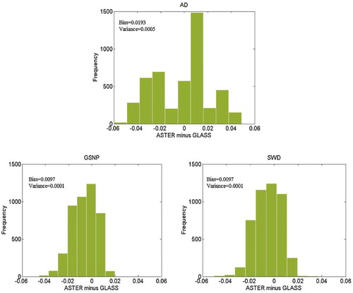
We downloaded the AST_05 and GLASS BBE datasets, which cover the in situ measurement sites, and then fused them using the MKF algorithm. The acquisition times of the ASTER emissivity products over sites Algodones Dunes (AD), Great Sands National Park (GSNP), and Stovepipe Wells Dunes (SWD) were 15 March, 18 March, and 30 April, 2008, respectively. The corresponding Julian days for the GLASS BBEs were 73, 81, and 121. The GLASS and ASTER BBE maps are shown in Figure 4; the purple blocks in the maps are the validation site locations. The BBEs varied from 0.85 to 1 over all the regions. The ASTER BBE contains more detailed information and gives clear textures of the different land cover types. Moreover, there are large differences between the GLASS and ASTER BBEs; the absolute values of the mean biases at sites AD, GSNP, and SWD were 0.0193, 0.0097, and 0.0097, respectively. Histograms for the three sites are shown in Figure 5.

Figure 4. Maps of the GLASS and ASTER BBEs before the MKF was applied.

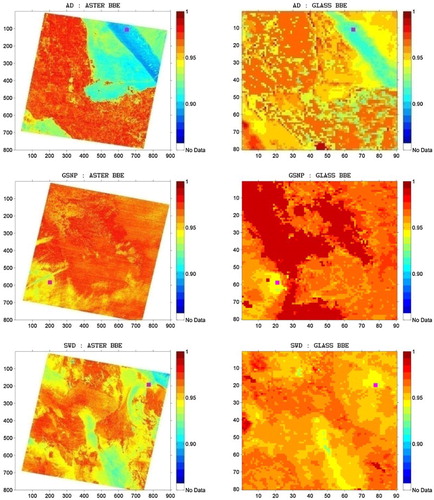
Figure 5. Histograms of the GLASS BBE minus the ASTER BBE for the three validation sites.

The MKF algorithm can provide estimates at different scales and individual results with different spatial resolutions, which is unlike the other data fusion or assimilation methods. The structure of the multi-resolution tree is shown in Table 3. The ASTER BBE was set to Scale 7, and the GLASS BBE was resampled to a 900-m spatial resolution using the nearest neighbour method and set to Scale 5.

Table 3. Multi-resolution tree structure.

Scale	Resolution	Pixels	Datasets
1	81 km × 72 km	1
2	40.5 km × 36 km	2 × 2
3	13.5 km × 18 km	6 × 4
4	4.5 km × 4.5 km	18 × 16
5	900 m × 900 m	90 × 80	GLASS BBE
6	180 m × 180 m	450 × 400
7	90 m × 90 m	900 × 800	ASTER BBE

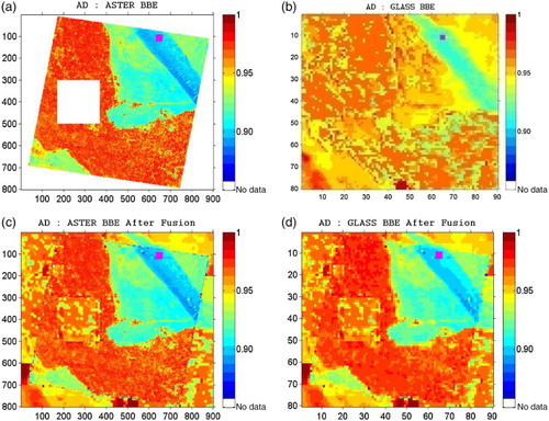
Herein, we will discuss site AD as an example. Figure 6 shows the comparison results before and after the fusion. The land cover mainly contains sand dunes, desert, and cropland, that is, the blue, green, and red coloured areas in the ASTER BBE map. Before the fusion, there were significant differences between the ASTER and GLASS BBEs at site AD, and the differences decreased after the fusion. The fused ASTER and GLASS BBEs had similar spatial patterns. Although the spatial resolution of the ASTER, BBE was higher than that of the GLASS BBE, ASTER cannot achieve global coverage because of its long revisit period (16 days) and narrow swath (60 km) (Cheng and Liang 2014c). Missing values or gaps always appear in composited regional and global BBE maps (Cheng and Liang 2014a). The MKF algorithm can be used to fuse multi-source data as well as for interpolation. As shown in Figure 6, the four corners of the original map contained no data; after fusion, those areas were filled with values, except for the boundary of the invalid data area. Moreover, the fusion also improved the quality of the maps, especially at the 900-m resolution. First, the smoothness of the 900-m resolution data was improved over that of the original map, and second, more detailed information from the 90-m resolution map was added to the 900-m resolution map. Note that there were no missing data in the ASTER images used in this study, but gaps in high-level optical remote sensing products due to clouds, for example, were common. The MKF algorithm can also fill in missing data in ASTER images, as demonstrated by the large block in Figure 7 in which a block of 200 × 200 pixels at site AD was set to zero. The block was filled with new data after the fusion; although the spatial pattern of the filled-in data in the ASTER image was similar to the corresponding area in the GLASS image, the filled-in data were different from those in the GLASS image. The fused value on each pixel was equal to the sum of a trend value and a random process estimate. According to Equations (8) and (9), the trend value was determined by the non-missing data (GLASS BBE) in the blank area, and the random process estimate was small compared to the trend value. Therefore, the trend value was the primary factor that determined the magnitude of the fused values. Therefore, although it seems that the filled data directly comes from the GLASS BBE, the values actually differed.

Figure 6. Maps of BBE at site AD before and after the fusion. (a) AD: ASTER BBE before fusion, (b) AD: GLASS BBE before fusion, (c) AD: ASTER BBE after fusion, and (d) AD: GLASS BBE.

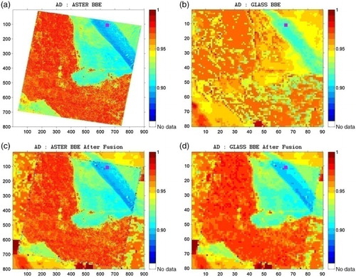
Figure 7. The fused results for site AD with missing data in ASTER images. (a) AD: ASTER BBE with missing data in a block of 200 × 200 pixels, (b) AD: GLASS BBE before fusion, (c) AD: ASTER BBE after fusion, and (d) AD: GLASS BBE after fusion.

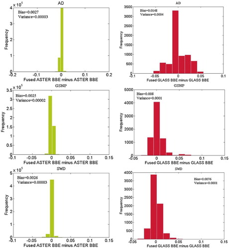
The histograms of the different BBE maps before and after fusion are displayed in Figure 8; the mean biases for the GLASS data were between 0.005 and –0.015 and were approximately three times larger than the mean bias of the ASTER difference. This is because the ASTER data are generally more reliable and the adjustment performed by the fusion process was smaller. Moreover, the biases for site AD with a 900-m resolution were much larger than those of the other two sites. Compared to the other sites, site AD has a more complex land cover of croplands, shrublands, and deserts, but sites SWD and GSNP mainly contain open shrublands.

Figure 8. Histograms of fused BBE minus original BBE.

In situ measurements collected at three sand dunes were used to validate the fusion results. The results are compared in Figure 9 and Table 4. At site AD, the error of the ASTER BBE was −0.0029 and was nearly identical after fusion (−0.0026). The error of the GLASS BBE changed from 0.0171 to 0.0003 after fusion. Clearly, the improvement in the GLASS BBE, which was 0.0168, was highly significant.

Figure 9. Site validation results.

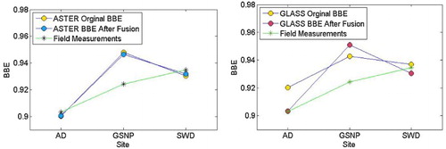
Table 4. Field validation results.

Sites	ASTER BBE before fusion	GLASS BBE before fusion	ASTER BBE after fusion	GLASS BBE after fusion	Field measurements
AD	0.9002	0.92015	0.9005	0.9034	0.9031
GSNP	0.9479	0.9428	0.9465	0.951	0.9242
SWD	0.9304	0.937	0.9296	0.9331	0.9347
Mean error	0.0103	0.01265	0.01	0.0096	−

The MKF improved the accuracy of the coarse data with relative lower accuracy in this case. Regarding site SWD, the ASTER and GLASS BBEs had higher accuracies. The errors were −0.0043 and 0.0023 before the fusion and −0.0051 and −0.0016 after the fusion, respectively. The potential improvement was small and may have even been slightly worse after the fusion.

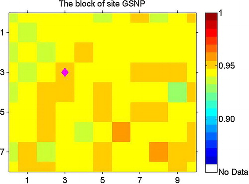
In contrast, the ASTER and GLASS BBEs had larger errors at the GSNP site, with values of 0.0237 and 0.0186, respectively. The errors were 0.0223 and 0.0268 after the fusion, respectively. These results are similar to the results at site SWD. In addition, it can be observed that the BBE after fusion at the GSNP site was 0.951 at the 900-m resolution. This value was larger than the original ASTER and GLASS BBEs, which were 0.9479 and 0.9428, respectively. Generally, the fusion result should be between the two original values. This anomaly was produced by spatial variability and the scale effect. The purple diamond in Figure 10 is the validation site. The pixels around the validation pixel in the 90-m resolution map show a large variability. Thus, all the pixels at 90-m and the BBE at the 900-m resolution were used to calculate the fusion result in the 90-m resolution map. All the child pixels in the same parent node were taken into account, not just the single pixel of the validation sites. Therefore, the scale effect and spatial variability require attention when trying to fuse two types of datasets at different spatial resolutions.

Figure 10. Site GSNP BBEs at the 90-m spatial resolution.

In summary, the MKF was able to improve the accuracy of the GLASS BBE when an accurate ASTER BBE and a relatively inaccurate GLASS BBE were fused. When the BBE datasets are either accurate or inaccurate, the improvement is either very limited or the results may even be slightly worse after fusion. The mean error of the sites at the 90-m resolution decreased from 0.0103 to 0.01, whereas the error of the data at the 900-m resolution was reduced from 0.01265 to 0.0096.

4.2. Comparison with other detrending methods

Because the MKF was designed to address random processes at different scales, the fusion methods using the MKF algorithm can only reduce measurements that include white noise. However, the BBE and other land remote sensing products often contain systematic and random measurement errors. It is very important to choose a proper detrending method to transform the dataset into a process that is suitable for the MKF. We applied two other methods (simple average and moving window) for comparison with the method proposed in this paper.

The simple average method removes the map’s mean value, and the entire map has a zero-mean to fit the state models. The moving window was used in He et al. (2014) and showed good efficiency. It uses a moving window as a filter and takes the filter result as the scale trend. The window size was determined by the multi-resolution tree. Figure 11 shows the fusion results for site AD using the simple average method. Obvious blocks can be observed on the left side of the map. These blocks can also be observed in the results of the other two methods, but they are less conspicuous. This drawback of the MKF has rarely been mentioned in previous studies, but it occurs because of the tree structure of the model. Although the pixels were adjacent, the fusion values of the pixels can have large differences because they belong to different parent nodes. Figure 12 shows the fusion results for the moving window method. The results have better visual continuity than those of the other two methods, but the fusion results at the 900-m resolution used only a small amount of information from the ASTER BBE map. This result is because the fusion results were greatly influenced by the detrending method and only used the moving filter result as the trend, and the trend, therefore, did not contain the ASTER BBE information. Comparative results for these two methods are presented in Table 5. The mean bias of the simple average method for the 900-m resolution was improved from 0.0126 to 0.0104. However, for the moving window method, the results for the 900-m and 90-m resolutions got worse.

Figure 11. Fusion result for the simple average detrending method.

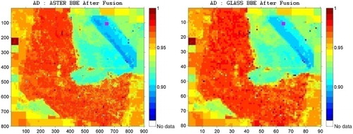
Figure 12. Fusion result for the moving window detrending method.

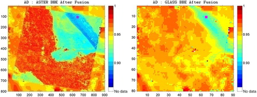
Table 5. Mean biases for the validation of the fusion results using other detrending methods.

Mean bias	ASTER BBE before fusion	GLASS BBE before fusion	ASTER BBE after fusion	GLASS BBE after fusion
Simple average	0.0103	0.01265	0.0104	0.0104
Moving window	0.0103	0.01265	0.0105	0.01445

5. Conclusions

Fusing multi-source information is an effective solution for improving the quality of high-level remote sensing products. The advantages of the MKF framework make it promising in the field of multi-resolution fusion problems, and it also avoids the computational efficiency problem. However, this framework has seldom been used in high-level land surface products.

In this paper, the MKF framework was utilized to fuse the GLASS and ASTER BBEs. An interpolation method to detrend the data was also proposed. The fused results demonstrated that the missing values in the high-resolution map were all filled and could generate spatially coherent BBE maps at different scales. The MKF can improve the accuracy of GLASS BBE when fusing accurate ASTER BBE and relatively inaccurate GLASS BEE. When the ASTER and GLASS BBEs are either accurate or inaccurate, the improvement is very limited or the results even may be slightly worse after fusion. The different detrending methods were also compared. The results showed that the simple average and moving window methods tended to produce more blocks in the results. The validation results indicated that our detrending method was better than the simple average and moving window methods. Moreover, the tests proved that the fusion result could be influenced by the detrending process.

In summary, the MKF method used in this study is capable of providing better estimates efficiently at different scales by fusing GLASS and ASTER BBEs with different spatial resolutions. Given these merits, this framework can be an alternative solution for estimating large land surface products, especially essential global land variables. In practice, special attention should be paid to the assumptions adopted in this framework. The trend and error variance of the trend should be carefully calculated because they are important background values that can influence later estimations. In this paper, we used the original framework to fuse two types of datasets; however, the assumptions in the MKF models are not well suited for land surface products. The framework should be further explored and adjusted to make it more universal, especially with regards to the models between the child and parent nodes. Moreover, attention should be given to the detrending methods because the MKF algorithm can only reduce the random measurement noise. Furthermore, it is very pertinent and important to extend this framework into a time–space multi-scale framework when dealing with assimilation problems and to test it using a large number of other products in various locations.

Acknowledgements

The authors would like to thank the MODIS website for providing the original products (http://reverb.echo.nasa.gov/reverb/). We would also like to thank Professor Paul W. Feiguth for answering some questions and providing the original codes on the website for reference.

Disclosure statement

No potential conflict of interest was reported by the authors.

Additional information

Funding

This work was supported by the National Natural Science Foundation of China [grant number 41371323] and the National High Technology Research and Development Program of China [grant number 2013AA121201].

Appendix 1. Estimator details of the MKF

The MKF procedure contains two sweep processes acting through the tree structure: a Kalman filter sweep and a Kalman smooth sweep. The prior value of the state and its variance are represented by and . The Kalman filter sweep begins at the finest scale to compute the filtered estimates, and is followed by the Kalman smooth sweep, which begins at the root node to compute the smoothed estimates and .

A.1. Kalman filter sweep

An initialization is required before starting the Kalman filter sweep process. For each node s at the finest scale, the initial state (a-priori values) is assigned to and . The following three steps are then executed:

1. Assimilate updating

This step assimilates the observational data to update the prior estimate: (A1) (A2)

where is an estimator gain given by (A3) (A4)

If is equal to zero, the measurements do not contribute additional information about the state. On the contrary, if is equal to unity, the measurement is perfect. If no measurements are available, the state and its variance are not updated.

• (2) Fine-to-coarse node updating

In this step, each node is updated from the fine scale to the coarse scale according to the state model. The children of node s are denoted by (A5) (A6)

• (3) Node blending

After updating all the nodes from the lower scale, all the child nodes must be integrated into the parent nodes. We specify here that each parent node has q child nodes: (A7) (A8)

The integrated estimate is a weighted sum of the estimates of its children. According to Equation (A8), the influence of the estimate in the integrating step decreases as the uncertainty in the estimate increases.

A.2. Kalman smooth sweep

After the Kalman filter sweep moves from the leaf nodes to the root node, the Kalman smooth process from the root node to the leaf nodes is used to obtain the optimal estimate. Using the result of the Kalman filter sweep, that is , with as the initial condition of the Kalman smooth and then combining with the upper scale data and prior variance, the results are given as (A9) (A10) where is a weighting coefficient, which is (A11)

References

- Bocchiola, D. 2007. “Use of Scale Recursive Estimation for Assimilation of Precipitation Data from TRMM (PR and TMI) and NEXRAD.” Advances in Water Resources 30 (11): 2354–2372. doi:10.1016/j.advwatres.2007.05.012.
- Bocchiola, D., and R. Rosso. 2006. “The Use of Scale Recursive Estimation for Short Term Quantitative Precipitation Forecast.” Physics and Chemistry of the Earth 31 (18): 1228–12239. doi:10.1016/j.pce.2006.03.019.
- Cheng, J., and S. Liang. 2013. “Estimating Global Land Surface Broadband Thermal-Infrared Emissivity from the Advanced Very High Resolution Radiometer Optical Data.” International Journal of Digital Earth 6: 34–49. doi: 10.1080/17538947.2013.783129
- Cheng, J., and S. Liang. 2014a. “A Comparative Study of Three Land Surface Broadband Emissivity Datasets from Satellite Data.” Remote Sensing 6: 111–134. doi: 10.3390/rs6010111
- Cheng, J., and S. Liang. 2014b. “Effects of Thermal-Infrared Emissivity Directionality on Surface Broadband Emissivity and Longwave Net Radiation Estimation.” IEEE Geoscience and Remote Sensing Letters 11 (2): 499–503. doi: 10.1109/LGRS.2013.2270293
- Cheng, J., and S. Liang. 2014c. “Estimating the Broadband Longwave Emissivity of Global Bare Soil from the MODIS Shortwave Albedo Product.” Journal of Geophysical Research-Atmosphere 119 (2): 614–634. doi: 10.1002/2013JD020689
- Cheng, J., S. Liang, W. Verhoef, S. Shi, and Q. Liu. 2016. “Estimating the Hemispherical Broadband Longwave Emissivity of Global Vegetated Surfaces Using a Radiative Transfer Model.” IEEE Transactions on Geoscience and Remote Sensing 54 (2): 905–917. doi:10.1109/TGRS.2015.2469535.
- Cheng, J., S. Liang, Y. Yao, and X. Zhang. 2013. “Estimating the Optimal Broadband Emissivity Spectral Range for Calculating Surface Longwave Net Radiation.” IEEE Geoscience and Remote Sensing Letters 10 (2): 401–405. doi: 10.1109/LGRS.2012.2206367
- Chou, K. C., and Massachusetts Institute of Technology Systems. 1991. “A Stochastic Modeling Approach to Multiscale Signal Processing.” Massachusetts Institute of Technology, Dept. of Electrical Engineering and Computer Science, N1 – 2012-04-17 16:08:00.
- Chou, K. C., A. S. Willsky, and A. Benveniste. 1994. “Multiscale Recursive Estimation, Data Fusion, and Regularization.” IEEE Transactions Automatic Control 39 (3): 464–478. doi: 10.1109/9.280746
- Chou, K. C., A. S. Willsk, and R. Nikoukhah. 1994. “Multiscale Systems, Kalman Filters, and Riccati-Equations.” IEEE Transactions Automatic Control 39 (3): 479–492. doi: 10.1109/9.280747
- Christakos, George, Alexander Kolovos, Marc L. Serre, and Fred Vukovich. 2004. “Total Ozone Mapping by Integrating Databases from Remote Sensing Instruments and Empirical Models.” IEEE Transactions on Geoscience and Remote Sensing 42 (5): 991–1008. doi: 10.1109/TGRS.2003.822751
- Dong, L. X., J. Y. Hu, S. H. Tang, and M. Min. 2013. “Field Validation of GLASS Land Surface Broadband Emissivity Database Using Pseudo-Invariant Sand Dunes Sites in Northern China.” International Journal of Digital Earth 6: 96–112. doi: 10.1080/17538947.2013.822573
- Duan, Q. Y., V. K. Gupta, and S. Sorooshian. 1993. “Shuffled Complex Evolution Approach for Effective and Efficient Global Minimization.” Journal of Optimization Theory and Application 3: 501–521. doi: 10.1007/BF00939380
- Fang, Hongliang, Shunlin Liang, Hye-Yun Kim, John R. Townshend, Crystal L. Schaaf, Alan H. Strahler, and Robert E. Dickinson. 2007. “Developing a Spatially Continuous 1 km Surface Albedo Data set Over North America from Terra MODIS Products.” Journal of Geophysical Research: Atmospheres 112 (D20): D20206. doi:10.1029/2006JD008377.
- Fang, H. L., S. L. Liang, J. R. Townshend, and R. E. Dickinson. 2008. “Spatially and Temporally Continuous LAI Data Sets Based on an Integrated Filtering Method: Examples from North America.” Remote Sensing of Environment 112: 75–93. doi: 10.1016/j.rse.2006.07.026
- Fieguth, P. W., W. C. Karl, A. S. Willsky, and C. Wunsch. 1995. “Multiresolution Optimal Interpolation and Statistical Analysis of TOPEX/POSITION Satellite Altimetry.” IEEE Transactions on Geoscience and Remote Sensing 33 (2): 280–292. doi: 10.1109/36.377928
- Fieguth, P. W., D. Menemenlis, T. Ho, A. Willsky, and C. Wunsch. 1998. “Mapping Mediterranean Altimeter Data with a Multiresolution Optimal Interpolation Algorithm.” Journal of Atmospheric and Oceanic Technology 15 (2): 535–546. doi: 10.1175/1520-0426(1998)015<0535:MMADWA>2.0.CO;2
- Gillespie, A. R., E. A. Abbott, L. Gilson, G. Hulley, J.-C. Jimenez-Munoz, and J. A. Sobrino. 2011. “Residual Errors in ASTER Temperature and Emissivity Products AST08 and AST05.” Remote Sensing of Environment 115: 3681–3694. doi: 10.1016/j.rse.2011.09.007
- Gillespie, A. R., S. Rokugawa, T. Matsunaga, J. S. Cothern, S. J. Hook, and A. B. Kahle. 1998. “A Temperature and Emissivity Separation Algorithm for Advanced Spaceborne Thermal Emission and Reflection Radiometer (ASTER) Images.” IEEE Transactions on Geoscience and Remote Sensing 36: 1113–1126. doi: 10.1109/36.700995
- Gottsche, F.-M., and G. C. Hulley. 2012. “Validation of six Satellite-Retrieved Land Surface Emissivity Products Over Two Land Cover Types in a Hyper-arid Region.” Remote Sensing of Environment 124: 149–158. doi: 10.1016/j.rse.2012.05.010
- Gupta, R., V. Venugopal, and E. Foufoula-Georgiou. 2006. “A Methodology for Merging Multisensor Precipitation Estimates Based on Expectation-Maximization and Scale-Recursive Estimation.” Journal of Geophysical Research 111 (D2): 93–108. doi:10.1029/2004JD005568.
- He, T., S. Liang, D. Wang, Y. Shuai, and Y. Yu. 2014. “Fusion of Satellite Land Surface Albedo Products Across Scales Using a Multiresolution Tree Method in the North Central United States.” IEEE Transactions on Geoscience and Remote Sensing 52 (6): 3428–3439. doi: 10.1109/TGRS.2013.2272935
- Huang, H. C., N. Cressie, and J. Gabrosek. 2002. “Fast, Resolution-Consistent Spatial Prediction of Global Processes from Satellite Data.” Journal of Computational and Graphical Statistics 11 (1): 63–68. doi: 10.1198/106186002317375622
- Hulley, G. C., and S. J. Hook. 2009a. “Intercomparison of Versions 4, 4.1 and 5 of the MODIS Land Surface Temperature and Emissivity Products and Validation with Laboratory Measurements of Sand Samples from the Namib Desert, Namibia.” Remote Sensing of Environment 113: 1313–1318. doi: 10.1016/j.rse.2009.02.018
- Hulley, G. C., and S. J. Hook. 2009b. “The North American ASTER Land Surface Emissivity Database (NAALSED) Version 2.0.” Remote Sensing of Environment 113 (9): 1967–1975. doi: 10.1016/j.rse.2009.05.005
- Hulley, G. C., S. J. Hook, and A. M. Baldridge. 2009. “Validation of the North American ASTER Land Surface Emissivity Database (NAALSED) Version 2.0 Using Pseudo-Invariant Sand Dune Sites.” Remote Sensing of Environment 113: 2224–2233. doi: 10.1016/j.rse.2009.06.005
- Jin, M., and S. Liang. 2006. “An Improved Land Surface Emissivity Parameter for Land Surface Models Using Global Remote Sensing Observations.” Journal of Climate 19: 2867–2881. doi: 10.1175/JCLI3720.1
- Kannan, Ashvin, Mari Ostendorf, William C. Karl, David A. Castañon, and Randall K. Fish. 2000. “ML Parameter Estimation of a Multiscale Stochastic Process Using the EM Algorithm.” IEEE Transactions on Signal Processing 48 (6): 1836–1840. doi: 10.1109/78.845950
- Li, A. H., Y. C. Bo, Y. X. Zhu, and P. Guo. 2013a. “Blending Multi-Resolution Satellite sea Surface Temperature (SST) Products Using Bayesian Maximum Entropy Method.” Remote Sensing of Environment 135: 52–63. doi: 10.1016/j.rse.2013.03.021
- Li, Z., B. Tang, H. Wu, H. Ren, G. Yan, Z. Wan, I. F. Trigo, and J. A. Sobrino. 2013b. “Satellite-derived Land Surface Temperature: Current Status and Perspectives.” Remote Sensing of Environment 131: 14–37. doi: 10.1016/j.rse.2012.12.008
- Li, Z.-L., H. Wu, N. Wang, S. Qiu, J. A. Sobrino, Z.-M. Wan, B.-H. Tang, and G.-J. Yan. 2013c. “Land Surface Emissivity Retrieval From Satellite Data.” International Journal of Remote Sensing 5: 1–44.
- Liang, S., K. Wang, X. Zhang, and M. Wild. 2010. “Review of Estimation of Land Surface Radiation and Energy Budgets from Ground Measurements, Remote Sensing and Model Simulation.” IEEE Journal of Selected Topics in Earth Observations and Remote Sensing 3 (3): 225–240. doi: 10.1109/JSTARS.2010.2048556
- Liang, S., X. Zhang, Z. Xiao, J. Cheng, Q. Liu, and X. Zhao. 2013a. Global LAnd Surface Satellite (GLASS) Products: Algorithm, Validation and Analysis. Beijing: Springer.
- Liang, S., X. Zhao, S. Liu, W. Yuan, X. Cheng, Z. Xiao, X. Zhang, et al. 2013b. “A Long-Term Global LAnd Surface Satellite (GLASS) Data-set for Environmental Studies.” International Journal of Digital Earth 6: 5–33. doi: 10.1080/17538947.2013.805262
- Menemenlis, D., P. Fieguth, C. Wunsch, and A. Willsky. 1997. “Adaption of a Fast Optimal Interpolation Algorithm to the Mapping of Oceanographic Data.” Journal of a Geophysical Research – Oceans 102 (C5): 10573–10584. doi: 10.1029/97JC00697
- Momeni, M., and M. R. Saradjian. 2007. “Evaluating NDVI-based Emissivities of MODIS Bands 31 and 32 Using Emissivities Derived by Day/Night LST Algorithm.” Remote Sensing of Environment 106 (2): 190–198. doi: 10.1016/j.rse.2006.08.005
- Ogawa, K., T. Schmugge, F. Jacob, and A. Prench. 2002. “Estimation of Broadband Land Surface Emissivity from Multi-Spectral Thermal Infrared Remote Sensing.” Agronomie 22: 695–696. doi: 10.1051/agro:2002055
- Ogawa, K., T. Schmugge, F. Jacob, and A. French. 2003. “Estimation of Land Surface Window (8–12 µm) Emissivity from Multi-Spectral Thermal Infrared Remote Sensing – a Case Study in a Part of Sahara Desert.” Geophysical Research Letters 30 (2). doi:10.1029/2002gl016354.
- Parada, L. M., and X. Liang. 2004. “Optimal Multiscale Kalman Filter for Assimilation of Near Surface Soil Moisture into Land Surface Models.” Journal of Geophysical Research 109 (D24). doi:10.1029/2004JD004745.
- Primus, I., D. McLaughlin, and D. Entekhabi. 2001. “Scale Rescursive Assimilation of Precipitation Data.” Advances in Water Resources 24: 941–953. doi: 10.1016/S0309-1708(01)00033-1
- Qin, J., S. Liang, X. Li, and J. Wang. 2008. “Development of the Adjoint Model of a Canopy Radiative Transfer Model for Sensitivity Study and Inversion of Leaf Area Index.” IEEE Transactions on Geoscience and Remote Sensing 46: 2028–2037. doi: 10.1109/TGRS.2008.916637
- Sabol, Jr. D. E., A. R. Gillespie, E. Abbott, and G. Yamada. 2009. “Field Validation of the ASTER Temperature-Emissivity Separation Algorithm.” Remote Sensing of Environment 113: 2328–2344. doi: 10.1016/j.rse.2009.06.008
- Salisbury, John W., Dana M. D’Aria, and Andrew Wald. 1994. “Measurements of Thermal Infrared Spectral Reflectance of Frost, Snow, and Ice.” Journal of Geophysical Research 99 (No. B12): 24235–24240. doi: 10.1029/94JB00579
- Simone, Giovanni, Alfonso Farina, Francesco Carlo Morabito, Sebastiano B Serpico, and Lorenzo Bruzzone. 2002. “Image Fusion Techniques for Remote Sensing Applications.” Information Fusion 3 (1): 3–15. doi: 10.1016/S1566-2535(01)00056-2
- Tustison, B., E. Foufoula-Georgiou, and D. Harris. 2002. “Scale-recursive Estimation for Multisensor Quantitative Precipitation Forecast Verification: A Preliminary Assessment.” Journal of Geophysical Research 107 (8377): 44–55. doi:10.1029/2001JD001073.
- de Vyver, H. V., and E. Roulin. 2009. “Scale-recursive Estimation for Merging Precipitation Data From Radar and Microwave Cross-Track Scanners.” Journal of Geophysical Research-Atmospheres 114. doi:10.1029/2008jd010709.
- Wang, D., and S. Liang. 2014. “Improving LAI Mapping by Integrating MODIS and CYCLOPES LAI Products Using Optimal Interpolation.” IEEE Journal of Selected Topics in Applied Earth Observations and Remote Sensing 7 (2): 445–457. doi: 10.1109/JSTARS.2013.2264870
- Zhou, L., R. E. Dickinson, Y. Tian, M. Jin, K. Ogawa, H. Yu, and T. Schmugge. 2003. “A Sensitivity Study of Climate and Energy Balance Simulations with use of Satellite-Based Emissivity Data Over Northern Africa and the Arabian Peninsula.” Journal of Geophysical Research 108 (D24): 4795. doi:10.1029/2003JD004083.
- Zhu, X. L., J. Chen, F. Gao, X. H. Chen, and J. G. Masek. 2010. “An Enhanced Spatial and Temporal Adaptive Reflectance Fusion Model for Complex Heterogeneous Regions.” Remote Sensing of Environment 114: 2610–2623. doi: 10.1016/j.rse.2010.05.032