The topological viewshed: embedding topological pointers into digital terrain models to improve GIS capability for visual landscape analysis

ABSTRACT

The effort to develop a Digital Earth has made dramatic progress in terms of visualisation and visual data integration for use-cases which demand semantically rich analysis. To provide this analysis and ensure legitimate representations of the spatial data from which visualisation are derived, it is necessary to provide more comprehensive analytical capabilities of the view. Questions of aesthetic valuation of landscape require a richer analytical response than simply ‘whether and possibly how much of’ an object or area of land can be seen. It requires interrogation of the scene as it appears and to distinguish between transient visual effects and those locally invariant to view point change. This paper explores a data structure to support scene analytics. As such, it first reviews the existing techniques from the fields of GIS and computer graphics as to their potential and limitations in providing a qualitatively more nuanced visual analysis. It then introduces a new method of encoding visually apparent relationships into terrain models. A prototype implementation is presented based on the Quad-Edge Triangular Irregular Network, though it is believed that raster or vector implementation would be possible. Although developed primarily with landscape analysis in mind, the method could have wider applicability.

KEYWORDS:

• Visibility
• analysis
• landscape
• topology
• viewshed

1. Introduction

Until recently, most GIS-based visual landscape analysis sought only to establish ‘whether  …  and possibly “how much of” [an object] is visible’ (De Floriani and Magillo 2003) not what it looks like, thus simple ray tracing to establish a binary viewshed map has proved largely sufficient. Techniques developed in computer graphics to handle the effects of perspective (e.g., the standard graphic pipeline) and thus provide information on the scene have not been widely adopted as an analytical method (i.e. as distinct from visualisation), because GIS users were not asking visibility questions which necessitated employing these more computationally expensive approaches.

Sang (2011) suggests the use of ‘visual topology’ as a means to address visual query of the scene. Sang, Hagerhall, and Ode (2015) demonstrate the perceptual salience of such visual–topological events. This paper implements a data structure which calculates visual topology and uses it to store a viewshed efficiently.

1.1. Evolving questions

The desirability of scene-specific analysis is not a novel problem in itself, having been previously addressed in theoretical terms (Marr 1982; Gibson 1986; Ervin and Steinitz 2003) and computationally (Bishop, Wherrett, and Miller 2000; Germino et al. 2001; Bishop 2003). However, GeoDesign (Wilson 2015) and digital globes mark a shift in both the technical approach and the user base (Goodchild 2008). Broader questions are being asked of geo-data by a broader range of people (the democratisation [Boulos and Burden 2007] or ‘google-isation’ [Infield 2009] of GIS). For example, inter-visibility might be sufficient for siting radio towers, but more nuanced information is needed for human perception of a viewshed (Ervin and Steinitz 2003; Chamberlain 2011; Nutsford et al. 2015) and the viewshed is only a partial picture of the scene (Ervin and Steinitz 2003; Sang, Ode, and Miller 2008; Sang, Hagerhall, and Ode 2015).

1.2. Evolving technology

While the questions have become more complex, computer graphics have become a mature technology; people can easily access 3D visualisations of their world and fast visibility analyses are available which extend questions beyond simple visibility (see Fisher [1996] for an overview and Sang [2016] for an updated review). It is relatively cheap to provide modelled, visualised images of future scenarios. This can be undertaken in online virtual worlds which (semi) automatically pull relevant data together. Once integrated with other technology, analytical nuance in query design may be lost, and the required expertise for understanding results is less apparent when data are interpreted via intuitive visualisation.

1.3. Evolving methodology?

Methods are needed to ensure that the data itself, as well as the technical and Spatial Data Infrastructure processes through which it is transformed for visualisation are fit for purpose (Sang 2011). For example, the developing field of landscape perception research places scientific demands on visual analysis (Nijhuis, van Lammeren, van der Hoeven, 2011).

The technical potential to handle ‘naïve’ queries which Egenhoffer and Mark called for (Egenhoffer and Mark 1995) needs to be addressed for an immersive ‘virtual world’ (Boulos and Burden 2007) to realise the potential of Digital Earth. For example, an ability to handle topological and spatial order queries (Egenhoffer 1989) in perspective would allow for more efficient handling of questions such as ‘how visually salient will a development be given its backdrop’. This could be important when human resources for Environmental Impact Assessment are limited (Vanderhaegen and Muro 2005).

1.4. Structure of the paper

Section 2 considers the need for a qualitatively nuanced visual analysis in the new Digital Earth and Internet-GIS era (Section 2.1); in particular, to address questions relating to a scene. It then considers the current capabilities and limitations of existing techniques from the fields of GIS and computer graphics with regard to these questions (Section 2.2). Section 3 introduces the key principles for a new method of encoding visually apparent relationships into terrain models. Section 4 sets out one particular approach to implementation. Section 5 then considers some possible areas of application and Section 6 discusses whether the proposed approaches support the visual analysis functions identified before Section 7 draws some brief conclusions.

2. Landscape view-analysis challenges

Sang (2011) set out several kinds of visual analytical processes for which current viewshed analysis provides only limited support:

1. Data integration; visualisation; and dynamic update.

2. Provision of metrics by individual view which may also account for spatial context in occluded areas of the scene.

3. Provision of summary metrics of landscape change.

4. Dynamic calculation of metrics along individual path choices.

5. Determination of representative viewpoints for an area.

6. Provision of information on the robustness of data for representing the view from a particular viewpoint, including issues of visualised scale relative to that of the original map data, and data heterogeneity within partially visible spatial units.

These have three basic technical requirements in common, the ability to establish:

1. How occluding horizons connect together in perspective view.

2. Which parts of the landscape are visible immediately beyond such horizons.

3. How (i) and (ii) change for changes in the model or viewpoint.

Occluding horizon topology (i) in the scene is a property which is absent from orthographically projected data (b, c, d), so summary metrics of this are useful both as landscape perception indicators (Sang, Hagerhall, and Ode 2015) and when determining representative viewpoints (e, f). Cross-horizon topology (ii) allows calculation of scene metrics which may differ from the viewshed (Sang, Ode, and Miller 2008) and thus processes (b, c, e) and is also relevant to path choice (d). The ability to track changes in the view (iii) is critical for dynamic update (a) as well as for viewpoints along a path (d). Lastly, tracking the occluding horizons spatially (i, iii) can also help determine when an update may be visually significant (f) and, as will be argued, whether it is appropriate to integrate multiple data sets within a scene given their different spatial units (a).

2.1. Traditional ray tracing vs. perspective graphics

Viewshed mapping (Figure 1) is the process of delineating on a map the areas which can or cannot be seen from a particular location. Two basic processes are commonly available for determining occluded areas: ray tracing (Watt 2002) and segment comparison (De Floriani and Magillo 2003; Madern et al. 2007). Until recently, the latter has rarely been used in GIS (one example being Madern et al. [2007]), primarily due to the ease of ray tracing on raster DEM.

Figure 1. A computer-generated scene (a) of the corresponding map (b) and viewshed (c) showing two land cover classes, for example, grassland (light green) and heather (dark green), in the viewshed (c) occluded area is blank. Arrows show field of view.

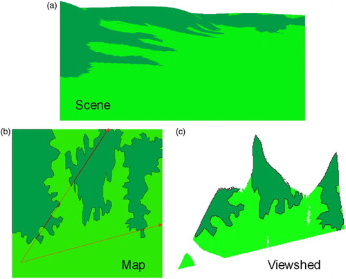
A more fundamental advantage of ray tracing for visibility analysis is the utility of the raster viewshed (Figure 1c) allowing objective measures and analytical summation but the technique has two key limitations. First, it does not provide the view, key details such as apparent landform are missing and the visible area may have holes and islands (Figure 1c). Second, the method is suited to a global approach rather than being built as a landscape is explored, analysing all data with what is a time-linear process at best (Reif and Sen 1988).

While variants of ray tracing can be used to provide qualitatively richer information, such as potential visual impact of buildings (Rød and Van Der Meer 2007), ‘visual dominance’ (Rana, 2003) and ‘visual magnitude’ (Chamberlain 2011), and can, of course, be used to visualise the scene, they do not provide an elegant solution for extracting quantitative metrics as to what the scene looks like (this paper being, perhaps, a first step towards such a solution).

Perspective visualisation is also a standard process. Graphical Projection is now routine (Angell 1981; Mortenson 1989) with efficient hidden surface removal (HSR) and rendering algorithms (Watt 2002). However, several of these efficiencies pose a number of problems for scientific landscape analysis.

Projection:

• Broad viewing angles (e.g., 360°) require a curved ‘screen’ against which to project objects so the benefit of hardware accelerated processing is harder to achieve than were a planar projection fustrum sufficient, though recent advances in Augmented Reality will hopefully reduce this issue.

• A ‘far clip frame’ (Turner 2003) may leave the topology of the remaining objects ambiguous (Leubke et al. 2002), a common solution, atmospheric fogging, may in fact be a variable of interest scientifically, for example, Bishop and Miller (2007).

• Floating point errors (due to there being a maximum resolution of any co-ordinate grid which perspective projections inevitably cut across [Worboys 1995, 188]). These may, in the worst case, be sufficient to create an error as to which object is nearer and which occluded during HSR (Sammet 1990, 267).

HSR:

• Predictable scene change (i.e., for story line efficiencies [Watt 2002, 357]) involves predetermination of what routes are followed, and what changes can be made to the model.

• Scene coherence (Watt 2002, 358) may reduce the number of ray traces needed in some areas but may also be a variable of scientific interest (Gibson 1986; Appleton 1996).

• The ‘painters algorithm’ (Sammet 1990, 271) produces a ‘dumb’ image where each layer painted is entirely unaware of what objects its colours represent and what objects it is painting over. In a ‘z buffer’ (Shirley et al. 2008), the direct link to the data, and thus its spatial topology, is also broken (Weghorst, Coppoer, and Greenberg 1984; see Watt 2002).

The issue of disconnecting perspective objects from the original data is, as far as the authors are aware, a fundamental limitation of all standard HSR methods which might be applied at a landscape scale. Both approaches share the fundamental problem of viewpoint-dependent Level of Detail. Graphical approaches have, perhaps, the advantage since ray-traced viewshed maps tend to assume perfect vision while the graphics pipeline can emulate the perspective-dependent acuity of the human eye. Proximate change in luminance and hue also affect visual salience to humans; thus, the ability to calculate both visual solid angle and perspective arrangement is important (Leubke et al. 2002, 239–278; Ogburn 2006).

2.2. Traditional viewshed mapping compared to the challenges

Before considering the theoretical issues raised by the challenges set out in Section 1.1, it is worth noting to what degree a traditional binary viewshed map and the ray tracing method of producing it meet those challenges:

1. Binary raster viewsheds are convenient for data integration since they provide for map overlay and raster calculations; however, they do not represent directly comparable data to that of the scene in a visualisation; one can expect differences in patch topology, size and shape (Sang, Ode, and Miller 2008).

2. The entire viewshed must be reconstructed for any change in landcover or viewpoint.

3. While landcover in a viewshed can be obtained by spatial overlay, perspective-dependent geometries and topologies, such as horizon intersections, are lost. ‘Screen dump’ visualisations of the scene provide the opposite problem whereby occluded information is lost; reclassification of the visible area from the screen is both slow and error prone.

4. Traditional rasters can provide summaries of landscape change with respect to the limited metrics they can measure, but perspective knowledge is required to provide information on whether that change is likely to be visually salient. Some variants have been proposed to supplement the raster viewshed with measures of visual dominance based on visual angle (Chamberlain 2011; Widjaja et al. 2015) and Bishop, Wherrett, and Miller (2000) use the Z-Buffer to determine visual depth, but this is largely at the pixel level.

5. Most visual metrics commonly calculated in orthographic projection – such as connectivity and shape complexity – are not presently supported for the scene (Ode, Hagerhall, and Sang 2010). Indeed, the lack of computational support could be one reason why few specifically scene-based metrics – such as visual topological complexity (Sang, Hagerhall, and Ode 2015) – have been proposed.

6. Traditional ray tracing analysis is too time consuming to provide a dynamic viewshed along a path though recent improvements such as Carver and Washtell (2012) achieve a binary viewshed in close to real time using the Graphical Processing Unit (GPU), and ESRI City Engine (ESRI 2013) might also be deployed to this end.

7. Determining a ‘representative’ scene requires many options to be considered. While Carver and Washtell’s (2012) approach will provide the necessary speed, scene topology might also play a role in scene perception (Sang, Hagerhall, and Ode 2015).

8. A binary viewshed may be compared with the original landcover by overlay to establish whether a landcover polygon in a visualisation is being partially occluded and thus one must consider if its landcover class remains correct. However, this is a separate operation from that of the visibility analysis itself. For a dynamic situation, it is arguably preferable to achieve both operations simultaneously, for example, when generating a visualisation ‘on the fly’ or designing reporting units for landcover maps which will be used in visualisation (Sang 2011).

9. In respect of dynamic changes in landform, such as when a forest is cleared, or grows substantially, it both changes the binary viewshed and becomes (in the case of growth) a new part of the visual landscape; this cannot be dealt with by overlay, but requires repeating the visibility analysis; yet, the viewshed does not provide the necessary information to identify when and where this might be necessary.

A more general problem is that analysing reporting units for visual factors (i.e., to minimise intra-unit heterogeneity for visual metrics) necessitates the connecting of knowledge of a unit in scene view, with that in orthographic view. At present, this must be achieved graphically, perhaps even requiring manual input (Germino et al. 2001; Sang, Ode, and Miller 2008). This makes it impossible to optimise units for multiple viewpoints, or relative to other landscape data, that is, to create a landcover map which reports relevant planning data along with scene characteristics in the same unit in order to allow planners to weigh visual factors into their decision-making (Grêt-Regamey, Bishop, and Bebi 2007).

3. Graphics-based landscape viewsheds and visual fields

3.1. Viewshed mapping by perspective graphics

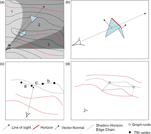
Landscape visual analysis provides one important option for efficiency; for a 2.5D manifold mesh, one can assume¹ that, when scanning from the view point outwards, any object with the same X co-ordinate in screen-space as a previously projected object, and lower Y co-ordinate in screen-space, must be occluded. Most of the cost of visibility analysis is in the intersection testing (Watt 2002, 355). If the geometry is not the cel² of the mesh but rather each cel’s bounding edge, intersect testing can be avoided except for those edges which, after approximate testing via the end nodes, might still intersect the current horizon, for example, line a–b Figure 2a (Madern et al. 2007).

Figure 2. (a) Maintaining a current horizon for HSR (inset shows horizon edge within TIN) and (b) the resulting information in orthographic and perspective views.

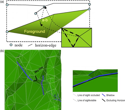
Given that occlusion testing is undertaken only against the current horizon, one should then note that it is the relationship between occluding horizons and the surface they partially occlude which is of interest. A map of the visible horizon edges (Fisher 1996), and the edges on which their shadows fall, completely describes the visibility of the land surface in between. So, rather than holding a viewshed as a separate layer with each object, cel, or raster-cell marked as visible or not, one could incorporate this horizon and shadow information as attributes of the digital terrain model (DTM). To determine visibility at any given point, one simply establishes if the first line intersected between that point and the viewpoint is an occluding horizon, and if so, the point is occluded, else it is visible (Figure 2b, see also De Floriani and Magillo (1996)).

3.2. Visual fields: variance in view analyses

Figure 3a shows the lines of sight for depth of view changes, while Figure 3b provides a side view. From this angle, it is possible to see how the lines of sight form a polygon or ‘visual hull’. This is not the same use of ‘visual hull’ as that defined by Laurentini (1991) in respect of visual object recognition (which is based on the silhouette projection of an entire object) but rather a reference to its similarity to the convex hull as commonly understood in computational geometry (Skiena 1998, 35) and GIS (Wright et al. 1996; Laurini and Thompson 1999, 587). The visual hull in this sense is useful as a special case of a visual field.

Figure 3. (a) Lines of sight to topological events in the scene and (b) the ‘visual hull’ they form spatially.

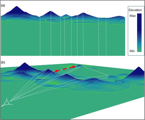
The concept of visual fields was first noted by Cova and Goodchild (2002) as a special case of field objects (Worboys 1995). In particular, Cova and Goodchild (2002) note the use of field objects to provide a greater insight into the range of options, whereby near-optimal solutions (e.g., mostly hidden) are also available rather than only the optimal solution. This means that whereas a viewshed provides one ‘snap shot’ against which the visibility or not of an object may be tested, the field object may be used for more subtle questions such as degree of visual salience. Thus, even if the ‘optimal’ solution would be that something is not visible, we may wish to test how close to that solution the actual case is, for example, ‘barely visible’.

It is this ability to investigate near-optimal solutions which also distinguishes the visibility graph (O’Sullivan and Turner 2001) from a standard viewshed analysis. Since the visibility graph represents all the viewsheds simultaneously as a matrix, variance in visibility within sub-regions of that matrix is also searchable (O’Sullivan and Turner 2001). However, O’Sullivan and Turner (2001) note that a key problem is selecting the objects in the landscape for which to construct the graph. They recognise that ‘the space complexity of this visibility graph data structure is O(kn) where k is the average size of each vertex neighbourhood’ (O’Sullivan and Turner 2001). Significantly, the visibility graph is only a topological field object; it records the inter-visibility between points, but not the geometry of that link in its spatial context. As a result, it has no means by which to ‘reverse the process of visibility graph construction – that is, many sets of locations in many environments could produce the same visibility graph, so that the environment so represented cannot be recovered from the visibility graph’ (O’Sullivan and Turner 2001). This also means that the process cannot be locally updated to take into account changes to a visual field due to altered geometry in the landscape.

Taking the concept of the visual field to that of a full geometrical object in the landscape would allow line-of-sight and apparent adjacency to be queried by traversing the edges of the visual field object as this would connect the landscape along lines-of-sight. Local changes could be detected by establishing if they are within a visual field object’s volume. The visual hull (Figure 3) could provide an object akin to a bounding box (Laurini and Thompson 1999, 126) or as a viewpoint-dependent convex hull (Wright et al. 1996), and be used as a preliminary test geometry to establish if a change requires a new visibility analysis.

3.3. Visual field to visual topology

The core problem is how to encode the perspective arrangement of the scene. How can one algorithmically identify from a DEM, and then map, features which are not in fact present at all, but result from human scene interpretation of a perspective view, for example, that horizons appear to intersect (Sang, Hagerhall, and Ode 2015)?

Two types of visual relationship can be distinguished; inter-visibility (along lines of sight as per a visibility graph) and ‘lateral-adjacency’ (which elements appear to be next to each other from a given perspective). The former was efficiently recorded by O’Sullivan and Turner (2001) but was not updatable. The latter has so far only been generally recognised as a property of the view in the field of Machine Vision (Plantinga and Dyer 1990) and has only been accessible in a landscape context by post hoc image analysis (e.g., via e-Cognition [Definiens 2011] or manually [e.g., Germino et al. 2001; Sang, Ode, and Miller 2005; Sang, Ode, and Miller 2008; Sang, Hagerhall, and Ode 2015]) which is both a slow process and also not easily updated.

Both types of visual relationship are hard to analyse because the visibility information has been removed from its spatial context. The visual field provides that spatial context, but managing this in a vector format would be computationally expensive (Haines 1994). For raster representations, the multiple scales and cross-axial vectors inherent in perspective operations could be problematic also, requiring some form of compression, for example, quadtree (Worboys 1995) to provide the higher resolution needed in some areas. Efficiency of storage and query becomes especially important if fuzzy viewsheds are of interest (Fisher 1994; Ogburn 2006). This work represents such relationships as a topological link between two points in the terrain (as per the dashed-line arrow in Figure 3).

Both inter- and lateral forms of visual topology are mediated by the same elements: horizons and their shadows. The proposed solution, therefore, is that rather than building visibility information in a separate map or matrix, the shadows and their respective horizons may be built into the primary data by setting pointers (memory address references) from one to the other.

4. Implementation in a Delaunay triangulated DEM

The implementation presented here is merely one means of achieving the general objective: to represent the scene as pointers within the DEM. The prototype was implemented in 2.5D for simplicity. After briefly introducing the Quad-Edge Triangular Irregular Network (TIN) data structure, the process will be explained as follows:

1. The TIN is ‘scanned’ from the viewpoint outward, that is, each edge is visited in distance order.

2. Edges are classified as to whether or not they are a potential horizon.

3. HSR is performed to see whether the edge is visible.

4. Pointers are set between horizons and the edges they occlude.

The Quad-Edge TIN has several aspects which recommend it for the purpose. TIN are well suited to represent visual fields as they provide both vector geometry and raster-cell topology at nested levels of complexity (Puppo 1996; Boots 1999; Mostafavi, Gold, and Dakowicz 2003). The resolution-variant properties of TIN are already used in most computer graphics applications where variable scale is important (Neves and Camara 1999).

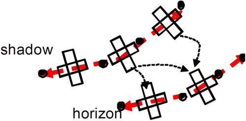
TIN edges are usually constructed by setting pointers between TIN nodes. Quad-Edge TIN also holds pointers to the triangle face. If the triangulation is Delaunay (1934), then these additional pointers describe the Voronoi diagram (the dotted lines in Figure 4a). The Voronoi diagram is useful as it is a fundamental form of natural neighbour spatial interpolation (Gold and Zhou 1990), and the frequent result of many anthropogenic and natural processes (Aurenhammer 1991). The Delaunay–Voronoi dual structure also provides the necessary criterion for various useful spatial operations via a simple set of operators (Guibas and Stolfi 1985; Aurenhammer 1991; Gold 2003; Mioc et al. 2007) in particular, a mesh scan which guarantees a distance ordered scan away from a point (Gold, Nantel, and Yang 1996).

Figure 4. (a) Quad-Edge Delaunay TIN and the Voronoi dual, and (b) embedding line of sight pointers. A ‘Quad-Edge’ (cross shape) is a set of four pairs of ‘Quads’ (squares). A Quad is a set of pointers. One pointer references the next Quad in the Quad-Edge, the other either points to one node at the end of the TIN edge (Green), or to one of the triangle faces either side (Red) – colours are greyed out for visually occluded quads. By following the pointers, it is possible to navigate the TIN.

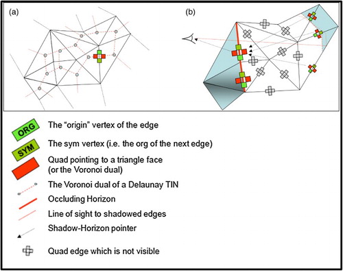
These aspects of the Quad-Edge TIN will be combined in order to identify lists (here after ‘chains’ to indicate their connected nature) of TIN edges which form occluding edges (horizons), or the boundary between occluded and non-occluded areas (shadow edges). In addition to the existing pointers that connect spatially adjacent TIN edges, pointers are added to connect TIN edges that appear adjacent from a particular viewpoint (Figure 4b). In this way, spatially separate ‘chains’ of horizons and shadows become connected together. The chains of pointers may be used to navigate the scene as it projects onto the map.

4.1. Building horizon–shadow chains

4.1.1. Scanning the mesh

Figure 5 illustrates the four stages in computing the pointers in Figure 4b. To identify the potentially relevant horizons, the mesh is scanned in three trees, as per the algorithm described in Gold, Nantel, and Yang (1996). The three-tone areas in Figure 5a (1,2,3) show the area to be scanned in numerical order away from the viewpoint. Thus, the edge between the two neighbouring triangles in Figure 5(a) would be dealt with before the more distant triangle.

Figure 5. (a) Scanning a mesh in three spirals, after Gold et al. (1996), (b) horizon determination, (c) visual intersection points, and (d) the horizon graph (note that shadow–horizon links need only be recorded when the shadowed edge is itself a horizon.

4.1.2. Horizon identification

Each edge forms the boundary between two neighbouring triangles. One is tested for back face culling first (Zhang and Hoff 1997) via vector normal comparison (Figure 5b). If not visible, it is ignored and the scan progresses. If visible, the neighbour is tested for backface culling. If this is not visible, then a horizon must exist between the two, the common Quad-Edge is marked as a potentially visible horizon (red line Figure 5b) but HSR must first be performed to determine if the edge is visible.

4.1.3. Hidden surface removal

Each edge is considered as a point pair. It is assumed that there are no ‘holes’ in the landscape. Figure 5c shows three possible cases for the projected lines a, b, c. If case (a), both points fall below the topmost previously processed edge, it is considered occluded and discarded. If case (b), both are above the top shadow and it is a horizon, it is added to a list of visible horizons along with its projected co-ordinates.

4.1.4. Pointer setting

If case (c), one point of the edge lies either side of the current horizon, the intersect is calculated and the geometry of the visible edge added to the list of horizons. But it is also given a pointer to the horizon which partially occludes it. The result is a ‘t-junction’ of the occluding and occluded horizon (Tarr and Kriegman 2001). This forces the horizon–shadow chain to split in three directions – edges to the left of the intersection, edges to the right and edges forming the intersecting ‘branch’.

As the dotted lines in Figure 5d illustrates, the horizon–shadow chains may form loops, creating a graph of occluding edges – on which visual Euler complexity is calculated by Sang, Hagerhall, and Ode (2015). ‘T-Junctions’ form nodes in the horizon graph (blue dots in Figure 5d). Between these nodes, the visibility or otherwise of edges in the graph is the same as its neighbours. It is not necessary to hold pointers between every shadowed edge in the graph and its occluding horizon that is implicit in the horizon graph. Only when visibility changes (at the nodes) is it necessary to set a pointer to explicitly record this in the TIN.

4.1.5. Pseudo code

The current maximal horizon can be maintained (as per Reif and Sen [1988]), so any point projected below this will not be visible. This HSR method also allows the horizon chain to be built:

//Set up a memory space (HList) to hold the memory address of each visible horizon edge identified (H) and its x,y co-ordinates on the view plane.//

 For each edge with starting node H1 and ending node H2;

    For a TIN segment S with starting node S1 and ending node S2;

    Project S1 and S2;

    If there is an element in HList where S1x or S2x between H1x and H2x

    //for long HList use divide and conquer as per Reif and Sen 1988//

       If S entirely below HList THEN End

        ELSE

          If S above HList THEN

            If horizon add to HList, Sort HList;

          End

          If S must intersect HList Then

            Add pointer to Quad;

            If horizon add to HList, Sort HList;

            If storing geometry calculate linear reference;

          End

       End

    End;

  Next

Next

4.1.6. Example

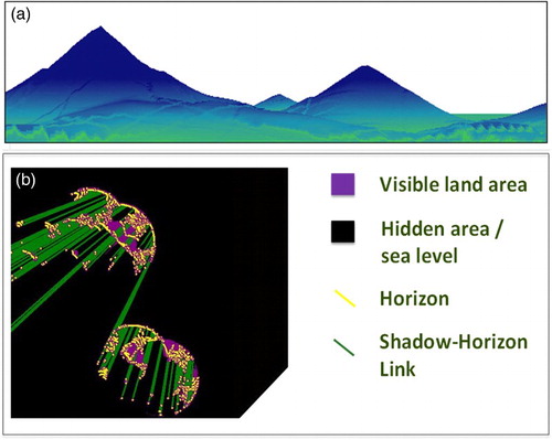
This method was implemented in VoronoiMagic, a Delphi-based software package for handling Quad-Edge Delaunay TIN, as a module ‘Landscape Information Tessellated Environment’ (VM-LITE); the full code can be found in Sang (2011). The scan method requires a Delaunay TIN, but the basic HSR and setting of pointers could in theory be applied to any vector-based data structure, while a raster structure could still deploy pointers but would require alternative HSR. Figure 6 shows the output from this, with a rendering of the data set in ArcGIS (Figure 6a) to give an impression of the terrain and the resulting map in VM-LITE (Figure 6b). The purple and black areas in Figure 6b are the visible and occluded areas of the viewshed respectively. The green lines show topological links between the horizon edges and those edges they shadow. They thus supplement the TIN topology to allow the scene to be traversed via the map, so scene metrics may be calculated directly without the need to reference a ‘screen dump’ image.

Figure 6. (a) Rendering of test data set in ArcGIS and (b) output from VM-LITE showing the viewshed (purple), horizons (yellow), and shadow–horizon links (green).

Using randomised height fields as test subjects, for a field of 100 points (roughly 500 triangles), with a height standard deviation of 18% using a standard laptop PC (Pentium 2 GHz dual core processor with 2 Gigabytes SD RAM), scanning the mesh and identifying horizons and their shadows took 2 seconds. Processing the data for a scene, such as that in Figure 6, with 250,000 points (77,000 of which were >0 heights, height SD 10%) took 28 minutes which compares reasonably to traditional ray tracing approaches (full test results are available in Sang [2011]).

More recent developments (Carver and Washtell 2012) are much faster, but it should be appreciated that this method was a prototype entirely implemented using the CPU to ensure complete control over the graphics pipeline; considerable speed improvements would be expected from involving the GPU. Furthermore, the product is not a simple viewshed but a map of how a scene is constructed. Such a map thus allows direct analysis of the scene but it also efficiently stores the scene such that certain kinds of scene change, for example, colour contrast, can be analysed without repeating the process. It can also be used to expedite subsequent visibility analysis for adjacent locations by ‘walking’ (i.e., iteratively moving) a horizon from its previous position until the correct new position is found (Sang (2011), 121) – this represents a time saving compared to assuming a full rescan is needed.

4.2. Storing horizon–shadow links

Pragmatically, the existing software base in Voronoi Magic provided a means of elegantly managing the quad-edge data structure. That the horizon–shadow chains would also be held using the quad-edge data structure did not necessarily follow. One option would have been a simple vector structure, calculating the intersect points for overlapping horizons and building a separate list. This could have been achieved by image analysis of the output graphics or from simple element-based visibility analysis (Madern et al. 2007). However, it would not provide any link to the original data. The entire process would need to be repeated for any minor change in landcover, viewpoint or landform. By embedding the links, landcover change can be queried in the scene, viewpoint change can be partially handled by the horizon walking process (Sang 2011), and landform change can be pre-tested against the visual hull.

To embed the horizon–shadow pointers into the Quad-Edge TIN, an occluding-horizon attribute is added to each Quad-Edge (Figure 7). As and when a horizon intersect is found, a pointer is set from this (the shadowed edge) to the horizon’s edge forming a line of sight from background to viewpoint. The entire visibility graph can thus be approximately encoded for one byte of memory per shadow–horizon intersection and one byte per horizon or shadow edge.

Figure 7. Embedding shadow–horizon links into a Quad-Edge TIN.

The solution is scalable between storage capacity and accuracy; thus, more accurate geometry can be encoded by providing linear references as to where on the respective edges the intersection falls. For the small overhead of bi-directional shadow–horizon pointers, the graph can be queried towards or away from viewpoints. Although not implemented here, the method can be extended to encode lists of pointers which simultaneously store Multiple-Linked View (sheds) and allow navigation between them, for example, to generate multi- and aggregate-visual impact metrics.

Since the VM-LITE prototype is only concerned with single viewpoints, a list is maintained to reference the shadow edges in the mesh (which in turn reference their respective horizons) and their projected/occluded perspective co-ordinates, to avoid the need for reprocessing this during analyses.

5. Applications

5.1. Attribute topology, landscape analysis, and data accuracy

The effect of perspective on visual characteristics can be established directly through querying the topological shadow–horizon links (yellow arrows in Figure 8). Figure 8 illustrates how patch size (Tveit, Ode, and Fry 2006) metrics in the view may not follow changes in spatial complexity as is often assumed (Sang, Ode, and Miller 2008). The true visual patch size (as viewed in perspective) can be calculated by using the shadow–horizon links to navigate between patches on the map that are adjacent in the view, summing their area if also visually indistinct from one another (Sang, Ode, and Miller 2008).

Figure 8. Landscape change as measured by patch count in viewshed (a, c) and scene (b, d).

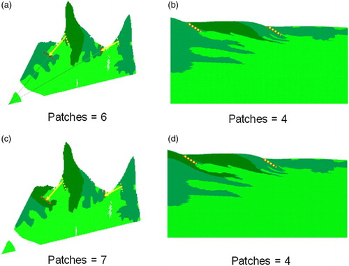
The yellow (upper) and red (lower) dotted lines show where far and near (respectively) landcovers apparently meet in the scene (Figure 8). In the case of Figure 8d, it can be seen that owing to the similarity of the landcover, this appears to be a single patch in the scene, but such is not the case in the viewshed. Of course, other aspects of view such as visual flow (Gibson 1986) may indicate the presence of a horizon between them, but this example demonstrates that the boundary may at best be a vague one. Another aspect of this arises from intra-unit heterogeneity (attributes that vary across a polygon); when only part of that area is also intersected by the visual field, the classification may be incorrect for the visible area. As the horizon–shadow provides pointers directly to the DTM, it is possible to detect when units are only partially visible and that Modifiable Area Unit Problems (Openshaw 1984) may need to be considered or even ecological fallacy (Laurini and Thompson 1999) due to a very unrepresentative ‘sliver’ polygon forming a substantial area on screen.

5.2. Landform analysis and change

The introduction of a structure to the landscape (e.g., a windfarm) may alter the content of the view (Figure 9a). This would be locatable with respect to the visual hull between a horizon and its shadow (Figure 9a) by constructing a plane.

Figure 9. (a) Establishing scene properties via shadow–horizon pointers, (b) scene framing effects, and (c) scene patch complexity.

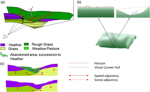
If a wind turbine is visible, the visual hull can be used to limit the area of the viewshed that needs re-calculating. Furthermore, the graph of the horizons provides a context to such changes, meaning visual impact analysis could be made more sensitive to local effects on individual viewpoints. For example, the proportion of a ‘framed view’ altered by the development could be calculated by adding the convex hull to the horizon graph (Figure 9b).

Non-geometric attribute changes are also easily established from the pointer structure. Figure 9c shows the impact in perspective if the rough grassland (the dotted area in Figure 9a) were to be abandoned and eventually succeed to heather. The dashed red lines in Figure 9a and Figure 9c are the same topological links. The solid red lines in Figure 9c are the spatially adjacent topology that would be measured by standard landscape metrics such as ‘contagion’ (McGarigal et al. 2002). Without the shadow–horizon links, the topology in the two images would need to be calculated through two separate analyses: ‘What is the spatial (e.g., ecological) topology’ and ‘what is the apparent scene topology’. In the former, the two landcover patches are separate; in the latter, they appear as a single patch. With the links, the perspective view is effectively ‘wired into’ the data set so the impact of a change in the map data on apparent patch size, contrast, richness and so on could be established almost instantly.

6. Discussion

To assess the proposed method, one may consider whether it holds the potential to meet the three technical requirements and relevant functions identified in Section 2.

Technical requirements:

1. The chain of horizons apparent in perspective view has been computed.

2. The cross-horizon topology of the view has been computed and efficiently stored.

3. The method provides for quickly detecting and analysing changes in the model, and for recording this information, including for multiple viewpoints if needed.

Functions:

1. To support integration; visualisation; and dynamic update.

As with the Quad-Edge TIN itself, more efficient methods may exist, for specific functions. However, the memory overhead seems likely to be acceptable for the added elegance of representation. The link between spatial analysis and visualisations is much stronger, in that the map allows query of the visualised scene in its spatial context and inclusion of dynamic update of the scene metrics with change in the attributes of the spatial land cover data.

1. Provision of metrics by individual view which may also account for spatial context in occluded areas of the scene.

Embedding the visual topology into the TIN provides the functionality of analysing characteristics in cross-horizon contrast or perspective-geometry that are highly specific to the viewpoint. Query of occluded areas adjacent to visible areas is also useful, for example, to consider the effects of uncertainty along the viewshed boundary.

1. Summary metrics of landscape change.

The horizons and shadows contain the topology of the horizon graph, and potentially its geometry also. In addition to visible and non-visible areas as available in standard, raster visibility maps, there is the potential to analyse visual complexity of horizons (Ode, Hagerhall, and Sang 2010; Sang, Hagerhall, and Ode 2015) and effects such as visual framing (Bell 1998), to add nuance to visual impact assessment.

1. Dynamic calculation of metrics along individual path choices

The line of sight pointers provide geometry (a visual hull) by which to test if a landscape change would be visible from previously processed viewpoints.

1. Determination of representative viewpoints for an area.

Section 3.2 makes the argument for the role of the visual field to investigate near-optimal solutions to a visibility query. Sang et al. (2015) also makes the case for the cognitive significance of horizon graph complexity and thus the need to consider them when determining a ‘representative’ viewpoint. The method presented here suggests a data structure that opens the visual field and the horizon boundaries to query from within its underlying spatial data.

1. Provision of information on the robustness of data for representing the view.

Since the shadow boundaries are mapped onto the 2D plane, it is possible to see where they fall in respect of other data sets such as land cover. One may thus automatically detect when, for example, a visualised scene is based on a sliver polygon resulting from the HSR and so identify when visualising this as the wider unit's landcover class would be an ecological fallacy.

The method relies on a geometric object model, and the implementation requires a Quad-Edge Delaunay TIN. While Quad-Edge-TIN hold many advantages, they are not generally supported by GIS. The underlying principle of setting pointers could be applied to any TIN model with some extra processing cost by the addition of a field for shadow–horizon pointers. Additional processing cost does, of course, pose a challenge to dynamic update, at least as regards viewpoint change, though one method to mitigate this through ‘walking horizons’ has been developed (Sang 2011).

The implementation in VM-LIGHT also uses the main Central Processing Unit to undertake the geometric calculations needed to construct the viewshed. This was a necessary compromise to ensure complete control over the graphics pipeline when developing the method; some steps might be far more efficiently achieved via the GPU. As Figure 6 shows, for more detailed DEM, the number of topological links to be managed can be large. For complex surface features, it may thus be of value to consider what kinds of visual topology are of principal interest, for example, only those pertaining to larger terrain features. This could be achieved through post process filtering. However, since only the topological relationships for visual intersections are recorded, the process scales with terrain complexity, not terrain resolution. The two are related, but terrain models with high resolution but large areas of simple morphology, will only generate shadow–horizon links in regions where the morphology is complex. This method is well suited to benefit from the multi-scale properties of TIN and means that much of the processing overhead in perspective intersection testing for locations which can be deduced as occluded may be avoided. Traditional raster viewsheds must calculate visibility for large areas of similarly positioned cells where visibility is impossible.

The final map from this process also represents a fraction of the memory required for a complete binary raster viewshed because the original underlying DTM is maintained with multiple viewsheds embedded as pointers therein. Not only does this avoid creating a complete surface for every view, but by allowing multiple views to be embedded into the DTM simultaneously, it also allows the scene to be reconstructed, some land cover changes incorporated without further recourse to perspective analysis, and common elements in multiple viewsheds to be semantically connected.

The TIN edges which are common to more than one scene represent an implicit link between them. The visual landscape is fundamentally one of different perspectives onto the same data, the cumulative effect of which is not the same as metrics on the terrain and land cover data as a single global entity. Problems of this nature are being increasingly acknowledged by the Digital Earth agenda via Multiple-Linked Views and Coordinated Multiple Views (CMV). Widjaja et al. (2015) deploy CMV to address simultaneous analysis and visualisation of multiple aspects and scales of data (i.e., metaphorical ‘points of view’). The principle is also true of literal viewpoints; indeed, one may not understand a system as perceived by one group without literally being able to see what they see in it, for example, why a development is seen as a visually dominant imposition on their community.

In respect of the choice of implementation in vector, raster, or triangulation, this of course depends on the wider technical and data ecology. DEM may traditionally be held as raster, but GIS is gradually merging with Computer-Aided Design models which are not easily converted to raster. Computer games, dominated by TIN, continue to drive the graphic fields, and are now sufficiently spatially aware to find roles in so-called ‘serious gaming’ (Poplin 2012) applications in participatory planning and citizen science. So, while Quad-Edge Delaunay TIN remains a niche data structure, with few implementations in 3D (see Ledoux (2006) for one), its comprehensive handling of cel and edge topology was an aid to prototyping. Perhaps that ability to replicate the functions of a raster, vector or TIN may yet see the Quad-Edge gain popularity as speed and flexibility take precedence, but if not, it at least provides proof of concept to the underlying idea. It must be acknowledged that the HSR implemented here relies on a 2.5D model of the terrain, while particular benefits of scene analysis over visibility analysis are likely to be found in urban areas, where more complex surface topology is to be expected. The pointer-setting method could still be applied in that circumstance and a full 3D model of Voronoi TIN has been implemented in the same software package used here (Ledoux 2006).

7. Conclusions

Modelling perceived visual relationships as topological relationships marks a substantial conceptual change in how the term topology is generally used in spatial science (and indeed mathematics). While Digital Earth has made great progress in visualisation and 3D visual data overlay (‘mash up’), analytical capabilities were slow to follow (Goodchild 2008) and recent progress (Veenendaal et al. 2014) relates primarily to 3D spatial modelling rather than perspective analysis. Yet, the capability to query data sets as they would be experienced in situ has implications far beyond that of how to handle perspective in landscape perception studies (Germino et al. 2001; Sang 2011; Sang, Hagerhall, and Ode 2015). The International Council for Science (ICSU) states that:

the requirements for Digital Earth are to provide a framework for shared global access to information .. to support scientific research, but also public participation in science.

ICSU: see Craglia et al. (2012)

In particular, to help personalise the ‘Grand Challenges’ ICSU identifies in terms of their relevance to different people, groups, and regions. Craglia et al. (2012) identify the need to develop ‘semantically rich descriptions of key concepts and processes, and underpinning assumptions’ including understanding ‘who wins and who loses’ under different scenarios, monitoring the perception of change, and the critical role of communicating uncertainty. The concept of visual topology is relevant in all of these respects. In natural language, we have a semantically rich set of descriptors for space (Mark and Egenhofer 1994), but visual relationships are not well translated into computational constructs. Lowering barriers to citizen engagement entails providing query functions able to recognise human perspective-based spatial constructs such as ‘what is that building visible just between the hills?’. In spatial planning, ‘who wins and who loses’ may often be line-of-site specific; for example, if one individual might lose their view of water or green space. More generally, the visual image of a change is an important factor in its perceived significance (O’Neill 2013), so obtaining an ‘objective’ or at least repeatable measure of what is seen would be important to calibrate citizen observations or identify when a visualisation is being selective. Identifying the appropriateness of a data set to visualisation is critical to communicating uncertainty and maintaining credibility (Appleton and Lovett 2003, 2005) and could also help generate feedback to improve data collection as part of Spatial Data Infrastructures for supporting visual analysis (Vanderhaegen and Muro 2005; Mohamadi et al. 2009).

The method proposed has considerable potential, allowing any processes which measure, monitor or optimise against scenic parameters to do so on the scene itself. This avoids the current division between rich analytical functions available on map data in orthographic view and the semantically limited information in perspective visualisations. The more comprehensive questions being asked, and the capabilities developed, perhaps demand that a distinction be made between ‘visibility analysis’ and ‘scene analysis’. Implementation in the more commonly used vector and raster formats is likely to be a pragmatic necessity if it is to be widely adopted; however, it is too early to make a cost–benefit comparison with simple visibility analysis because many of the more semantically demanding use-cases are only now beginning to be identified. Ultimately, it is hoped that such an approach would allow SDI to better support quality assurance, naïve query and perspective analytics as visual modelling becomes an increasingly important end use for spatial data.

Acknowledgements

The authors would like to acknowledge the Macaulay Development Trust for funding the PhD (undertaken at the University of South Wales) of which this work formed a part. This work was partly funded by the Rural & Environment Science & Analytical Services Division of the Scottish Government. Special thanks are also due to Dr Maciej Dackowicz and all those who helped to create the Voronoi Magic software upon which VM-LITE was built.

Disclosure statement

No potential conflict of interest was reported by the authors.

ORCID

N. Sang http://orcid.org/0000-0002-7722-9618

Notes

1. Unless the terrain were to contain tunnels or bridges, in which case a simple additional operation can be employed to establish visibility. If the point is found to be below an existing line, one can check whether the area in the view below that horizon is solid by querying the vector normal of the potentially occluding triangle’s neighbour. If it is groundward, the horizon must be the edge of a tunnel or depression. However, for now, the simpler case will be assumed.

2. A ‘cel’ refers to a single projected object once any part which is occluded has been removed, it is not a mis-spelling of the word ‘cell’.

References

- Angell, I. 1981. A Practical Introduction to Computer Graphics. London: Macmillan Press.
- Appleton, J. 1996. The Experience of Landscape, Revised Edition. New York: Wiley and Sons.
- Appleton, K., and A. Lovett. 2003. “GIS based Visualisation of Rural Landscapes: Defining Sufficient Realism for Environmental Decision Making.” Landscape and Urban Planning 65 (3): 13–31. doi: 10.1016/S0169-2046(02)00245-1
- Appleton, K., and A. Lovett. 2005. “GIS-Based Visualisation of Development Proposals: Reactions from Planning and Related Professionals.” Computers, Environments and Urban Systems 29 (3): 321–339. doi: 10.1016/j.compenvurbsys.2004.05.005
- Aurenhammer, F. 1991. “Voronoi Diagrams – A Survey of a Fundamental Geometric Data Structures.” ACM Computing Surveys 23: 345–405. doi: 10.1145/116873.116880
- Bell, S. 1998. Landscape: Pattern, Perception and Process. London: E & FN Spon.
- Bishop, I. 2003. “Assessment of Visual Qualities, Impacts, and Behaviours, in the Landscape, by Using Measures of Visibility.” Environment and Planning B: Planning and Design 30: 677–688. doi: 10.1068/b12956
- Bishop, I., J. Wherrett, and D. Miller. 2000. “Using Image Depth Variables as Predictors of Visual Quality.” Environment and Planning B: Planning and Design 27: 865–875. doi: 10.1068/b26101
- Bishop, Ian D., and D. Miller. 2007. “Visual Assessment of Off-Shore Wind Turbines: The Influence of Distance, Contrast, Movement and Social Variables.” Renewable Energy 32 (5): 814–831. doi:10.1016/j.renene.2006.03.009
- Boots, B. 1999. “Spatial Tesselations.” In Geographic Information Systems, Volume 1, Principles and Applications, edited by P. A. Longley, M. F. Goodchild, D. J. Magiure, and D. W. Rhind, 503–536. New York: Wiley.
- Boulos, M. N. K., and D. Burden. 2007. “Web GIS in Practice V: 3-D Interactive and Real-time Mapping in Second Life.” International Journal of Health Geographics 6: 51. doi:10.1186/1476–072X-6–51. Accessed January 19, 2010. http://www.ij-healthgeographics.com/content/6/1/51. doi: 10.1186/1476-072X-6-51
- Carver, S., and J. Washtell. 2012. “ Real-time Visibility Analysis and Rapid Viewshed Calculation Using a Voxel-based Modelling Approach.” GIS Research UK 2012, April 11–13, Lancaster, UK.
- Chamberlain, B. 2011. Toward Human-Centered Approaches in Landcape Planning; Exploring Geospatial and Visualisation Techniques for the Management of Forest Aesthetics. Vancouver: University of British Colombia.
- Cova, T. J., and M. F. Goodchild. 2002. “Extending Geographical Representation to Include Fields of Spatial Objects.” International Journal of Geographic Information Science 16 (6): 509–532. doi: 10.1080/13658810210137040
- Craglia, Max, Kees de Bie, Davina Jackson, Martino Pesaresi, Gábor Remetey-Fülöpp, Changlin Wang, Alessandro Annoni, et al. 2012. “Digital Earth 2020: Towards the Vision for the Next Decade.” International Journal of Digital Earth 5 (1): 4–21. doi:10.1080/17538947.2011.638500
- Definiens. 2011. “ Definiens XD 1.5.2 Release Notes.” In Definiens AG, Trappentreustraße 1, 80339 München, Germany. Accessed July 26. http://www.definiens.com.
- De Floriani, L., and P. Magillo. 1996. “Representing the Visibility Structure of a Terrain Through a Nested Horizon Map.” International Journal of Geographical Information Systems 10 (5): 541–562. doi: 10.1080/02693799608902096
- De Floriani, P., and P. Magillo. 2003. “Algorithms for Visibility Computation on Terrains: A Survey.” Environment and Planning B – Planning and Design 30 (5): 709–728. doi: 10.1068/b12979
- Delaunay, B. 1934. “Sur la sphère vide. Classe des Sciences Mathématiques et Naturelle.” Bulletin of the Academy of Sciences of the U.S.S.R., 7, 6: 793.
- Egenhoffer, M. 1989. A Formal Definition of Binary Topological Relationships, Lecture Notes in Computer Science. London: Springer-Verlag.
- Egenhoffer, M., and D. Mark. 1995. Naïve Geography, COSIT ‘95, Semmering Austria. Edited by A. W. Kuhn Frank, Vol. 988, Lecture Notes in Computer Science. New York: Springer-Verlag.
- Ervin, S., and Steinitz, C. 2003. “Landscape Visibility Computation: Necessary, but not Sufficient.” Environment and Planning B: Planning and Design 30: 757–766. doi: 10.1068/b2968
- ESRI. 2013. ESRI City Engine – A New Dimension. Redlands, CA: ESRI Press. http://www.esri.com/library/ebooks/a-new-dimension.pdf.
- Fisher, P. 1994. “Probable and Fuzzy Models of the Viewshed Operation.” In Innovations in GIS 1, edited by M. F. Warboys, 161–175. London: Taylor and Francis.
- Fisher, P. 1996. “Extending the Applicability of Viewsheds in Landscape Planning.” Photogrammetric Engineering and Remote Sensing (PE&RS) 62 (11): 1297–1302.
- Germino, M., W. Reiners, B. Benedict, D. McLeod, and C. Bastian. 2001. “Estimating Visual Properties of Rocky Mountain landscapes Using GIS.” Landscape and Urban Planning 53: 71–83. doi: 10.1016/S0169-2046(00)00141-9
- Gibson, J. 1986. The Ecological Approach to Visual Perception. Hillsdale, NJ: Erlbaum Associates.
- Gold, C. 2003. “Primal/Dual Spatial Relationships and Applications.” Proceedings 9th International Symposium on Spatial Data Handling, sec. 4a. http://citeseerx.ist.psu.edu/viewdoc/download?doi=10.1.1.1.4728&rep=rep1&type=pdf.
- Gold, C., J. Nantel, and W. Yang. 1996. “Outside-in: An Alternative Approach to Forest Map Digitizing.” International Journal of Geographical Information Science 10 (3): 291–310. doi: 10.1080/02693799608902080
- Gold, C., and Zhou, F. 1990. Spatial Statistics on Voronoi Polygons. http://www.voronoi.com/wiki/images/6/63/Spatial_statistics_based_on_Voronoi_polygons.pdf.
- Goodchild, M. F. 2008. “The Use Cases of Digital Earth.” International Journal of Digital Earth 1 (1): 31–42. doi:10.1080/17538940701782528
- Grêt-Regamey, A., I. Bishop, and P. Bebi. 2007. “Predicting the Scenic Beauty Value of Mapped Landscape Changes in a Mountainous Region through the Use of GIS.” Environment and Planning B, 34: 50–67. doi: 10.1068/b32051
- Guibas, L., and J. Stolfi. 1985. “Primitives for the Manipulation of General Subdivisions and the Computation of Voronoi.” ACM Transactions on Graphics 4 (2): 74–123. doi: 10.1145/282918.282923
- Haines, E. 1994. “Point in Polygon Strategies.” In Graphics Gems IV, edited by Paul Heckbert, 24–46. San Diego, CA: Academic Press. From Draft. Accessed July 26 2011. http://erich.realtimerendering.com/ptinpoly/.
- Infield, N. 2009. “SLA Europe Event – The Google-isation of [Re]search.” Accessed January 19, 2010. http://britishlibrary.typepad.co.uk/inthroughtheoutfield/2009/10/sla-europe-event-the-googleisation-of-research.html (Permalink).
- Laurentini, A. 1991. “ The Visual Hull: A New Tool for Contourbased image Understanding.” In Proceedings of the 7th Scandinavian Conference on Image Analysis, 993–1002. Aalborg, Denmark.
- Laurini, R., and D. Thompson. 1999. Fundamentals of Spatial Information Systems. London: Academic Press.
- Ledoux, H. 2006. “Modelling Three-dimensional Fields in Geoscience with the Voronoi Diagram and its Dual.” University of Glamorgan, UK.
- Leubke, D., M. Reddy, J. Cohen, A. Varshney, B. Watson, and R. Huebner. 2002. Level of Detail for 3D Graphics. Amsterdam: Morgan Kaufman.
- Madern, N., M. Fort, N. Madern, and J. Sellares. 2007. “Multi-Visibility of Triangulated Terrains.” International Journal of Geographic Information Systems 21 (10): 1115–1134. doi: 10.1080/13658810701300097
- Mark, D. M., and M. J. Egenhofer. 1994. “Calibrating the Meanings of Spatial Predicates from Natural Language: Line-region Relations.” Spatial Data Handling 1: 538–553.
- Marr, D. 1982. Vision: A Computational Investigation into the Human Representation and Processing of Visual Information. San Fransisco, CA: Freeman.
- McGarigal, K., S. Cushman, M. Neel, and E. Ene. 2002. “FRAGSTATS: Spatial Pattern Analysis Program for Categorical Maps. Computer Software Program Produced by the Authors at the University of Massachusetts.” Amherst. Accessed September 26, 2011. www.umass.edu/landeco/research/fragstats/fragstats.html.
- Mioc, D., F. Anton, C. M. Gold, and B. Moulin. 2007. “Voronoi Diagrams in Science and Engineering.” In SVD apos 07 4th International Symposium on Voronoi Diagrams, 135–144, Glamorgan, UK. July 9–11, Permalink. Accessed September 26, 2011. http://ieeexplore.ieee.org/servlet/opac?punumber=4276089.
- Mohamadi, H., A. Rajabifard, A. Binns, and I. Williamson. 2009. “Multi-Source Spatial Data Integration within the Context of SDI Initiatives.” International Journal of Spatial Data Infrastructures Research 4: 18.
- Mortenson, M. 1989. Computer Graphics: An Introduction to the Mathematics and Geometry. New York: Industrial Press.
- Mostafavi, M., C. Gold, and M. Dakowicz. 2003. “Dynamic Voronoi/Delaunay Methods and Applications.” Computers & Geosciences 29 (4): 523–530. doi: 10.1016/S0098-3004(03)00017-7
- Neves, N. J., and A. Camara. 1999. “Virtual Environments and GIS.” In Geographic Information Systems, Volume 1, Principles and Applications, edited by M. F. Goodchild, P. A. Longley, D. J. Magiure, and D. W. Rhind, 557–567. London: Wiley.
- Nijhuis, S., R. van Lammeren, F. van der Hoeven. 2011. “Exploring the Visual Landscape.” Research in Urbanism 2, 978-1-60750-832-8 (print) | 978-1-60750-833-5 (online). http://ebooks.iospress.nl/volume/exploring-the-visual-landscape.
- Nutsford, D., F. Reitsma, A. Pearson, and S. Kingham. 2015. “Personalising the Viewshed: Visibility Analysis from the Human Perspective.” Applied Geography 62: 1–7. doi: 10.1016/j.apgeog.2015.04.004
- Ode, Å., C. Hagerhall, and N. Sang. 2010. “Analysing Visual Landscape Complexity: Theory and Application.” Landscape Research 35: 111–131. doi: 10.1080/01426390903414935
- Ogburn, D. 2006. “Assessing the Level of Visibility of Cultural Objects in past Landscapes.” Journal of Archaeological Science 33: 405–413. doi: 10.1016/j.jas.2005.08.005
- O’Neill, Saffron J. 2013. “Image Matters: Climate Change Imagery in US, UK and Australian Newspapers.” Geoforum 49: 10–19. doi:10.1016/j.geoforum.2013.04.030
- Openshaw, S. 1984. The Modifiable Areal Unit Problem. Vol. 28, Conceptual Techniques in Modern Geography. Norwich: Geo Books.
- O’Sullivan, D., and A. Turner. 2001. “Visibility Graphs and Landscape Visibility Analysis.” International Journal of Geographical Information Science 15: 221–237. doi: 10.1080/13658810151072859
- Plantinga, H., and Dyer, C. 1990. “Visibility Occlusion and the Aspect Graph.” International Journal of Computer Vision 5 (2): 136–160. doi: 10.1007/BF00054919
- Poplin, Alenka. 2012. “Playful Public Participation in Urban Planning: A Case Study for Online Serious Games.” Computers, Environment and Urban Systems 36 (3): 195–206. doi:10.1016/j.compenvurbsys.2011.10.003
- Puppo, E. 1996. “Variable Resolution Triangulations.” In Technical Report n.6/96. Genova: Istituto per la Matermatica Applicata, Consiglio Nazionale delle Ricerche.
- Rana, S. 2003. “Fast Approximation of Visibility Dominance using Topographic Features as Targets and the Associated Uncertainty.” Photogrammetric Engineering and Remote Sensing 69: 881–888.
- Reif, J., and S. Sen. 1988. “An Efficient Output-Sensitive Hidden Surface Removal Algorithm and Its Parallelization.” In Annual Symposium on Computational Geometry, Proceedings of the 4th Annual Symposium on Computational Geometry, 193–200. Champaign, IL: Urbana-Champaign.
- Rød, J. K., and D. Van Der Meer. 2007. “Visibility and Dominance Analysis: Assessing a High Building Project in Trondheim.” ScanGIS 07, Aas, Norway.
- Sammet, H. 1990. Applications of Spatial Data Structures. Vol. Computer Graphics, Image Processing and GIS. Reading, MA: Addison-Wesley.
- Sang, N. 2016. “Wild Vistas: Progress in Computational Approaches to ‘Viewshed’ Analysis.” In Mapping Wilderness: Concepts, Techniques and Applications, edited by J. Stephen Carver and Steffen Fritz, 69–87. Dordrecht: Springer Netherlands.
- Sang, N. 2011. “Visual Topology in SDI: A Data Structure for Modelling Landscape Perception.” University of South Wales, UK.
- Sang, N., C. Hagerhall, and Å. Ode. 2015. “The Euler Character: A New Type of Visual Landscape Metric?” Environment and Planning B: Planning and Design 42 (1): 110–132. doi: 10.1068/b38183
- Sang, N., Å. Ode, and D. Miller. 2005. “Visual Topology for Analysing Landscape Change and Preference.” In Proceedings of the 17th Annual Meeting of ECLAS Landscape Change, Ankara, Turkey, 176–185. September 14–18.
- Sang, N., Å. Ode, and D. Miller. 2008. “Landscape Metrics and Visual Topology in the Analysis of Landscape Preference.” Environment and Planning B 35: 504–520. doi: 10.1068/b33049
- Shirley, P., K. Sung, E. Brunvand, A. Davis, S. Paker, and S. Boulos. 2008. “Education: Fast Ray Tracing and the Potential Effects on Graphics and Gaming Courses.” Computers and Graphics 32: 260–267. doi: 10.1016/j.cag.2008.01.007
- Skiena, S. 1998. The Algorithm Design Manual. New York: Springer-Verlag.
- Tarr, M., and D. Kriegman. 2001. “What Defines a View?” Vision Research 41: 1981–2004. doi: 10.1016/S0042-6989(01)00024-4
- Turner, A. 2003. “Analysing the Visual Dynamics of Spatial Morphology.” Environment and Planning B 30 (5): 641–796. doi: 10.1068/b12962
- Tveit, M., A. Ode, and G. Fry. 2006. “Key Concepts in a Framework for Analysing Visual Landscape Character.” Landscape Research 31 (3): 229–255. doi:10.1080/01426390600783269
- Vanderhaegen, M., and E. Muro. 2005. “Contribution of a European Spatial Data Infrastructure to the Effectiveness of EIA and SEA Studies.” Environmental Impact Assessment Review 25 (2): 123–142. doi: 10.1016/j.eiar.2004.06.011
- Veenendaal, Bert, Songnian Li, Suzana Dragicevic, and Maria Antonia Brovelli. 2014. “Analytical Geospatial Digital Earth.” International Journal of Digital Earth 7 (4): 253–255. doi:10.1080/17538947.2014.896967
- Watt, A. 2002. 3D Computer Graphics. 3rd ed. New York: Addison-Wesley.
- Weghorst, H., G. Coppoer, and D. Greenberg. 1984. “Improved Computational Methods for Ray Tracing.” ACM Transactions on Graphics 11 (2): 214–222.
- Widjaja, Ivo, Patrizia Russo, Chris Pettit, Richard Sinnott, and Martin Tomko. 2015. “Modeling Coordinated Multiple Views of Heterogeneous Data Cubes for Urban Visual Analytics.” International Journal of Digital Earth 8 (7): 558–578. doi:10.1080/17538947.2014.942713
- Wilson, Matthew W. 2015. “On the Criticality of Mapping Practices: Geodesign as Critical GIS?” Landscape and Urban Planning 142: 226–234. doi:10.1016/j.landurbplan.2013.12.017
- Worboys, M. 1995. GIS A Computing Perspective. London: Taylor and Francis.
- Wright, M., A. Fitzgibbon, P. J. Giblin, and R. B. Fisher. 1996. “Convex Hulls, Occluding Contours, Aspect Graphs and the Hough Transform.” Image and Vision Computing 14 (8): 627–634. doi: 10.1016/0262-8856(96)01100-6
- Zhang, H., and K. Hoff. 1997. “Fast Backface Culling Using Normal Masks.” In Symposium on Interactive 3D Graphics Archive, Proceedings of the 1997 Symposium on Interactive 3D Graphics, 103–106. Providence, RI, USA.