A variable precision rough set approach to knowledge discovery in land cover classification

ABSTRACT

This paper presents a granular computing approach to spatial classification and prediction of land cover classes using rough set variable precision methods. In particular, it presents an approach to characterizing large spatially clustered data sets to discover knowledge in multi-source supervised classification. The evidential structure of spatial classification is founded on the notions of equivalence relations of rough set theory. It allows expressing spatial concepts in terms of approximation space wherein a decision class can be approximated through the partition of boundary regions. The paper also identifies how approximate reasoning can be introduced by using variable precision rough sets in the context of land cover characterization. The rough set theory is applied to demonstrate an empirical application and the predictive performance is compared with popular baseline machine learning algorithms. A comparison shows that the predictive performance of the rough set rule induction is slightly higher than the decision tree and significantly outperforms the baseline models such as neural network, naïve Bayesian and support vector machine methods.

KEYWORDS:

• Rough set theory
• soft computing
• granular computing
• remote sensing
• approximate reasoning

1. Introduction

In recent years, there is a growing interest in understanding the uncertainty aspect of spatial data modeling and processing beyond a classical approach (Allard 2013; Beaubouef and Petry 2013; Griffith, Wong, and Chun 2016; Hong et al. 2014; Kinkeldey 2014; Pogson and Smith 2015; Sikder 2008). The representation of space in terms of idealized abstraction of geometric primitives (e.g. polygons, lines and points) offers a limited and inadequate approach to understand the complex spatial distribution of the dynamic process. Underlying in these concepts are the crisp boundary sets that constitute the domain of decision. In practice, the assumption is not well founded that the ‘real’ boundary is an objective entity and that with precise and accurate measurement these boundaries can be represented with certain degree of error. For example, the classification of remote sensing imagery or suitability measures of a land parcel for a given use depends on the process of driving classification schemes or preference schemes in relation to certain spatial properties (such as neighborhood) as well as non-spatial attributes (Aggarwal 2015; Han, Kamber, and Pei 2012; Miller and Han 2009; Sikder 2010). However, a classification scheme has to deal with the notion of the likelihood of the presence or absence of a concept in a given spatial object defined by some boundary definition. Therefore, the question ‘where does a forest begin?’ is not only a topological or geometric question, it is also a question of semantic classification (Morris et al. 2010). Many of these problems related to uncertainty stem from representation of space in terms of idealized abstraction of geometric primitives in crisp boundary sets constituting the domain of decision. Moreover, the classification scheme also depends on a set of evidence from the supporting data set which are very often derived from multiple sources (e.g. from satellites, dispersed hyperspectral sensors or aerial photography) at varying degrees of quality and scale. Therefore, it is necessary to understand how the attributes of spatial objects or evidences suggesting various conceptual or thematic classifications can be understood in a broader approach to allow objective classification by considering the uncertainty intrinsic in the spatial application models and decision processes. Ignoring the intrinsic complexities of spatial properties may result in misinterpretation. There is inadequate support to represent and characterize uncertainty when the resource analysts and managers are required to extract knowledge and induce semantic classification in complex geospatial evidences. Therefore, conventional geographic information systems (GIS) or RS processing and machine learning models need specialized attention when dealing with spatial entities (Banerjee, Carlin, and Gelfand 2014; Shekhar, Kang, and Gandhi 2009; Vinh and Le 2012).

This paper presents a ‘soft computing’ formalism to deal with uncertainty inherent in spatial data in terms of rough set-based toleration relations which can be used to characterize, predict and assess the accuracy of land cover classification. It provides a new methodology to discover empirical knowledge in multi-source supervised land cover classification under uncertainty stemming from imprecision as well as inconsistency within the thematic spatial layers. The methodology provides rich and extensible schema for interpreting semantics in spatial data and classification in terms of quantifiable uncertainty parameters and associated domain rules and corresponding features.

In the following sections, we first provide the role of rough set theory in knowledge induction. We develop a characterization method of classification to approximate within variable precision domain. We also present an empirical validation and prediction methodology using remotely sensed data and ancillary biophysical data set. Finally, we present a comparison of predictive performance with baseline machine learning algorithms such as a decision tree (C4.5), support vector machine (SVM), an artificial neural network and a naïve Bayesian method.

1.1. Related works

The characterization of the spatial relationships between remotely sensed imagery with biophysical parameters is an important aspect of understanding the dynamics of land cover and land use processes (Perez et al. 2016; Serra, Pons, and Saurí 2008; Song et al. 2014). Various studies have identified that spatial integration of social and biophysical factors aid in better understanding of land cover models as well as changes (Brown et al. 2004; Evans and Moran 2002; Straume 2014; Thackway, Lymburner, and Guerschman 2013). A common aspect of these efforts requires multi-source data fusion within varying spatial and temporal resolutions. In remote sensing, multi-source data fusion problems have been well studied (Amarsaikhan et al. 2012; Gamba 2014; Zhang 2010). Despite increasing attention, there still remain many challenges. Most importantly, the issue of the scale effect in the model constructs still remains a significant challenge (Masek et al. 2015; Sheppard and McMaster 2008; Turner et al. 1989; Weng 2014; Wu and Li 2009). The scale effects have been studied with respect to fractals as mathematical model for spatial variation (Feng and Liu 2015; Jiang and Brandt 2015; Riccio and Ruello 2015), geostatistical model for scaling up and down (Atkinson 2001; Wang et al. 2016) and modifiable areal unit problem (MAUP, Lin et al. 2013). In addition to the spatial scale, uncertainty could emerge from classification schemes and classification errors (Lechner et al. 2012). The issues of data quality in spatial prediction due to inaccuracy and imprecision and effects of discrete spatial representation and spatial error propagation have been receiving increasing attention in recent years (Brus and Pechanec 2015; Guptill and Morrison 1995; Harvey and Leung 2015; Robertson et al. 2014; Zandbergen et al. 2012). Uncertainty in spatial databases has been addressed in many different aspects, for example, quality and meaning of data, representation of multiple resolutions, communicating spatial model context, generalization of environmental models, propagation of errors in spatial analysis and multi-source classification and knowledge discovery of geographic features (Hunsaker et al. 2013). Conventionally available GISs offer fusion operations such as maps overlay and weighted linear combination that are essentially based on Boolean logic (Malczewski 2006). The attributes of spatial objects or evidences suggesting various conceptual or thematic classifications need to be understood in a broader context to incorporate the notion of the approximation of classification. In order to overcome the Boolean constraints, fuzzy set theory and rough set theory have been employed to manage spatial objects with uncertain or intermediate boundaries (Beaubouef and Petry 2010; Gao, Wu, and Gao 2007; Petry and Elmore 2015). However, in fuzzy logic the membership function of an object to a given fuzzy concept requires some a priori mathematical function. While in rough set theory, the membership function is directly computed from the given data without requiring any distribution assumption. The feature reduction algorithm offered in rough set theory makes it uniquely attractive to reduce the curse of dimensionality, for example, remote sensing feature selection or band selection in hyperspectral imagery (Patra, Modi, and Bruzzone 2015; Zhao and Pan 2015). Rough set theory has also been used to extract complex spatial relationships (Ge et al. 2011a) and spatio-temporal outlier detection (Albanese, Pal, and Petrosino 2012). As a successor to rough set theory, the VPRS offers further generalization to allow partial or probabilistic classification (Xie, Lin, and Ren 2011). Thus, it provides additional levels of confidence in land cover classification. The application of VPRS is reported to provide a meaningful method to discriminate confusing objects (e.g. to different specific vegetation from water bodies) in remote sensing imagery (Xie, Lin, and Ren 2011). Also, to overcome the sensitive dependence of the spectral variation of between-class and within-class, the VPRS offers tolerance subset operators through the inclusion of error measure (Pan et al. 2010).

2. Research method

This paper uses classical rough set theory and its extension VPRS. It is based on an empirical knowledge discovery and classification scheme that emphasizes the implication of granularity inherent in the data set in handling imprecise and vague information. Since the methodology uses an extended form of rough set theory, the methodology and the algorithm inherit the inherent data-driven and non-invasive nature of rough set theory and its computational efficiency. The research method includes several phases: research analysis and design, data preparation, empirical application of the model, comparison and with baseline model, and interpretation and implication application of the research output. Figure 1 outlines the overall research workflow. Broadly, it includes multi-source data integration within GIS/RS and rough set framework. VPRS is used to characterize the uncertainty parameters by introducing approximation measures in the accuracy parameters of land cover classes. To validate the rough set learning framework, the data set is partitioned into training set (66%) and testing set. The rough set rule induction generates decision rules from the training set which is applied on the testing set to predict.

Figure 1. A general diagram for research procedure. The ovals represent data set (input/output) and rectangles represent processes or algorithm.

Finally, the prediction accuracy is compared with the baseline algorithm (decision tree – C4.5), neural network, naïve Bayesian and SVM methods. The subsequent sections explain the detailed descriptions of the steps.

2.1. Knowledge induction and rough set theory

As a part of the ‘soft computing’ paradigm, rough set is regarded as a ‘non-invasive’ way of formalization of uncertainty (Düntsch and Gediga 1998; Pawlak 2002; Sikder and Munakata 2009). Rough set was introduced to characterize a concept in terms of elementary sets in an approximation space. Information granulation or the concept of indiscernibility or granularity is at the heart of rough set theory. Classical rough theory and it extensions have been widely used in real-world applications machine learning, remote sensing, satellite image processing and many more related disciplines. Modified rough set theory has been used to retrieve land use/land cover from remote sensing imagery (Lei, Wan, and Chou 2008; Leung et al. 2007; Pan et al. 2010; Xie, Lin, and Ren 2011; Yun and Ma 2006). Classical rough set allows one to characterize a decision class in terms of elementary attribute sets in an approximation space. Spatial categories can be represented in the form , where is the decision attribute or the thematic feature such as ‘forest’ in a given location and U is the closed universe which consists of non-empty finite set of objects (a number of spatial categories) and C is a non-empty finite set of attributes that characterizes a spatial category, that is, ‘forest’ such that for every c ∈ C, is a value of attribute c. This is achieved by means of information granulation or indiscernibility is at the heart of rough set theory. A finer granulation means more definable concept. For , the granule of knowledge about a forest with respect to indiscernibility relation can be represented as follows:(1) Thus, the locations x and are indiscernible from each other if and the decision about the presence or absence of ‘forest’ in a given location is approximated by lower and upper approximation of decision concept as follows:(2) (3) Thus, the objects in can be classified with certainty as the ‘forest’ on the basis of knowledge in B, while the objects in can be only classified as the possible occurrence of forest and the boundary region () represents the uncertainty in decisive classification.

Since in real world, it is difficult to identify all possible attributes causing species incidence or propagation, it will be necessary to establish a methodology to identify the critical attributes by eliminating redundant attributes using feature reduction or knowledge compression methods in rough set knowledge systems. This can be achieved by removing the attributes whose removal will not change the indiscernibility relation. A discernibility function is represented as follows:

It represents the prime implicants of candidate attributes () generating the minimal set of attributes also known as reduct. While computing prime implicants is an NP-Hard (Pawlak and Skowron 2007) problem, it is possible to use heuristic algorithm (Li, Mei, and Lv 2011; Yang et al. 2013) (e.g. dynamic reducts – Trabelsi, Elouedi, and Lingras 2011; Xu, Wang, and Zhang 2011), genetic algorithm (Huang 2012; Sarkar, Sana, and Chaudhuri 2012) or particle swarm optimization (Bae et al. 2010; Ding, Wang, and Guan 2012) to generate a computationally efficient set of minimal attributes. Furthermore, it is possible to discover the degree of dependency of the attributes to uncover causal inference of the land cover formation process. The advantage is that the output will provide a mathematically rigorous means to trace or back track the causal links of the land cover dynamics. The rough set knowledge induction process can be implemented within multi-layer GIS to incorporate qualitative knowledge in the knowledge induction process. Thus, the rules induced by the rough set knowledge discovery process can be regarded as a data pattern that represents relationship between multiple thematic layers in GIS and qualitative knowledge. The minimal set of satisfactory rules will provide the means to generate a predictive surface where the risk of invasion can be mapped easily. The rules can also provide new insights about the potential impact of some ecological and human-induced social factors that may have long-term impacts in inter-specific interactions. Table 1 illustrates an example of fictitious readings at different locations or granular units of knowledge set.

Table 1. A decision system in rough set.

Locations	Temp	Moisture	Soil depth	Forest type
S1	Low	Low	High	A
S2	Low	Low	High	A
S3	High	Low	High	D
S4	Low	High	Low	B
S5	Low	High	Low	C

In this case, we can define the following partitions based of the indiscernibility relations: IND ({Temp, Moisture, Soil Depth}) = {S1, S2}, {S3}, {S4, S5}}, as shown in Table 2.

Table 2. Equivalence classes.

	Temp	Moisture	Soil depth
E1: [S1, S2]	Low	Low	High
E2: [S3]	High	Low	High
E3: [S4, S5]	Low	High	Low

A discernibility matrix defines each equivalence class with respect to one row and column. For a set of attributes in (U, A), the discernibility matrix M_T(B) is an n × n matrix such thatwherefor i, j = 1,2,  … , n.

Table 3 shows a symmetric discernibility matrix where each entry in the matrix represents attributes, the value of which renders the equivalence classes different.

Table 3. The discernibility matrix.

	E1	E2	E3
E1	Ø
E2	{Temp}	Ø
E3	{Moisture, SoilDepth}	{Temp, Moisture, SoilDepth}	Ø

2.2. Discernibility function

Using the discernibility matrix, it is possible to calculate the reducts or most important attributes of the information systems. The discernibility function f_A for an information system is a Boolean function defined as follows:

where n = |U/IND(B)|, and a disjunction is taken for all set of Boolean variable corresponding to the element of discernibility matrix. For example, the discernibility function of the above information system is:

The prime implicants of f_A provide the minimal subsets of attributes.

2.3. Reducing attributes: reducts

A reduct represents an attribute subset B ⊆ A of an information system such that after removal of an attribute/s from an equivalence class, it preserves indiscernibility relation. In other words, all attributes in a reduct are indispensable. The set of several such minimal attributes are called reducts. The set of prime implicants of the discernibility function determines the reducts.

Using the discernibility function, we can determine the reducts of previous example. Each function is then minimized in product form:

Therefore, reducts are: Reduct 1 = {Temp, Moisture}, Reduct 2 = {Temp, SoilDepth}

2.4. From reducts to rules

Rules are generated from reducts in the form: α→β, read as ‘if α then β’ where the antecedent (α) represents the set of conditions or set of conjunctive attributes and corresponding values and the consequent (β) represents the decision class or their disjunction. Transforming reducts to rules involves linking the attribute value of the object from which reducts are generated to the correspondent attributes of the reduct. From the previous example, the derived reducts can be used to extract the following rules:

R1: Temp (Low) AND Moisture (Low) ForestType (A)

R2: Temp (High) AND Moisture (Low) ForestType (D)

R3: Temp (Low) AND Moisture (High) ForestType (B) OR ForestType (C)

R3: Temp (Low) AND SoilDepth (High) ForestType (A)

R4: Temp (High) AND SoilDepth (High) ForestType (D)

R5: Temp (Low) AND SoilDepth (Low) ForestType (B) OR ForestType (C)

Using these rules, it is now possible to classify new instances of forest type.

2.5. Approximation evaluation by granularity measures: variable precision rough sets

The partition induced by the equivalence classes can be mapped with a different set of decision classes and to their lower and upper approximations. The set of objects that certainly are members of a class are assigned to the lower approximation region. The upper approximation is a set consisting of objects that are possibly members of a class with respect to the attributes or given knowledge. The difference between the upper and lower approximation is the boundary region or the region of uncertainty. The rough set defined in this sense is based on the concept of total membership function. In a variable precision rough set (Mi, Wu, and Zhang 2004; Ziarko 2012), the definition of lower and upper approximations is referred with respect to a variable precision where the lower and upper approximations are a special case:

By using rough memberships, the lower and upper approximations can be generalized to arbitrary levels of precision . This is based on the concept of the boundary region thinning of the variable precision model where we can look at the distribution of decision values within each equivalence class, and exclude those decisions having a lower frequency threshold of . In this case, the lower frequency decision values can be treated as ‘noise’. Furthermore, the concept of sensitivity and specificity can be used to evaluate the approximation (Komorowski and Øhrn 1999). These evaluation parameters are defined as follows:

Sensitivity indicates the number of objects correctly approximated as members divided by the actual number of members, that is, the proportion of the positives. While specificity is the measures of proportion of negatives, that is, interpreted as the number of object correctly approximated as non-members divided by the actual number of non-members. The overall accuracy is defined as the ratio of total number of correctly approximated object to the total number of objects. The overall accuracy is measured by weighting between sensitivity and specificity:

3. Empirical validation and prediction

The empirical substantiation of the theory is established in a supervised classification of multi-attribute geographic data. We have applied the model in a real-world application where environmental land cover classes are regarded as the response decision class conditioned by attribute structure, for example, environmental and human factors.

3.1. Data description and preprocessing

The study area has been chosen as a subset of the Hindu Kush Himalayan (HKH) region, which includes 231 × 128 pixels with geographic coordinates ranging from 33.22°N to 31.97°N in latitude and 68°E to 70.29°E in longitude. The decision classes are the land cover classes from satellite remote sensing images, and the attributes used are biophysical evidences (see Table 4) suggesting a land cover classes, which are derived from the global land cover data set developed by IGBP (International Geosphere–Biosphere Program) (Loveland et al. 2000). The data set is a product of the initiative of the U.S. Geological Survey's (USGS) Earth Resources Observation System (EROS) Data Center, the University of Nebraska-Lincoln (UNL) and the Joint Research Center of the European Commission. In connection with the land cover characterization effort of the National Aeronautics and Space Administration’s (NASA) Earth Observing System Pathfinder Program, the project generated a 1-km resolution global land cover database suitable for use in environmental research and modeling applications. The data set is derived from 1-km Advanced Very High Resolution Radiometer (AVHRR) data spanning a 12-month period (April 1992–March 1993) and is based on a flexible database structure and seasonal land cover regions concepts. The method used to derive these classes involves a multi-temporal unsupervised classification of NDVI data with post classification refinement using multi-source earth science data (Loveland et al. 2000). Monthly AVHRR NDVI (Normalized Difference Vegetation Index) maximum value composites were used to define seasonal greenness classes which were then translated to seasonal land cover regions by post-classification refinement with the addition of ancillary eco-region data and a collection of other land cover/vegetation reference data. For this study, the original classes of the data set were aggregated and regrouped into some general category to represent board-level classes. These are cropland, forest, grassland and shrub, dry or sparsely vegetated. The land cover classes of the study area show relatively uneven distribution in each class. The class label ‘a’, ‘b’, ‘c’, ‘d’ and ‘e’ represent ‘shrub’, ‘grassland’, ‘forest’, ‘cropland’ and ‘desert’, respectively. Henceforth, the encoded class labels are used in place of their original labels.

Table 4. The summary of conditioning attributes.

Attribute	Description	Value description
Digital elevation model (DEM)	Elevation	Numerical
Length of growing period (LGP)	Indicator of available moisture – when precipitation exceeds half the potential evapotranspiration	Numerical
Mean annual temperature (ATMP)	Mean annual temperature	Numerical
Slope (SLP)	Slope – derivative of DEM	Numerical
Population density (PDEN)	Population density – raster grid surface	Numerical
Distance to nearest road (RDIST)	Euclidean distance function of road network – represents accessibility index	Numerical
Land cover class (CLS)	Derived from multi-seasonal cluster of NDVI image	Categorical
Soil depth	Weighted average of the depth class and partial area covered in each soil mapping unit	Categorical

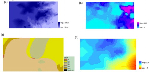
The digital terrain model is derived from the Digital Chart of the World of Environmental Systems Research Institute’s (ESRI) the digital contour map of 1000-ft. intervals. Based on the Delaunay triangulation algorithm, a Triangulated Irregular Network (TIN) was generated from contour data incorporating streamline coverage as break line for interpolation. The TIN was then converted to raster continuous surface. The raster representation of the grid data set of the area has a spatial resolution of 1 km. The experiment considers land cover classes as the decision class, and the combination of biophysical attributes indicates the evidences in support of a set of land cover class for a given pixel. The geographic layers of the attribute data set were resampled and projected to a common coordinate system to spatially register the same land cover class of a given pixel with the corresponding attribute values. The climatic data sets were derived from the Digital Water and Climate Atlas for Asia – a research project output initiated by Utah Climate Center of Utah State University. The data source is based on point interpolation of station data. The algorithm used for interpolation is based on a minimum curvature multi-dimensional splining technique. The precipitation surfaces were derived similarly from the same data source, calculated as the sum of all daily precipitation for each grid node for monthly and annual values. Following a water balance model developed by FAO (1978–1981), the length of growing period is derived by calculating the period (in days) during the year when precipitation exceeds half the potential evapotranspiration. However, where temperature is too low (<5°C of mean annual temperature) for crop growth, the growing period was not taken into account. Socio-economic data, in particular the raster demographic database, is derived from the global population data set, which is an output of a project carried out as a cooperative activity among NCGIA, CGIAR and UNEP/GRID. The procedure used to develop this database is the redistribution of population totals for the administrative unit in proportion to the accessibility index for each grid cell. The basic assumption upon which the construction of population distribution raster grids for Asia is based is that population densities are strongly correlated with accessibility. The population density surface was then resampled to match with the rest of the data set of the study area. Additionally, a cost distance grid surface was developed from the Euclidean distance function of the road network of the area to represent an accessibility index. The data for the location of roads were derived from the vector database contained in the Digital Chart of the World. Figure 2 illustrates sample feature attributes.

Figure 2. Sample feature attributes: (a) elevation derived digital elevation model; (b) population density; (c) soil depth; and (d) mean annual temperature.

3.2. Attribute discretization

Rough set theory usually requires categorical or discrete attributes in a given decision table. Assigning a single attribute class to a spatial element or ‘object’ is necessary when mapping the decision variable with an attribute variable in an information system. Hence, the rasterized elements are to be assigned with discrete attribute classes by means of discretization. The effect of discretization is the alteration of the granularity because of ‘coarsening’ the view of perception of the analysis. The effect of discretization methods on the rough set-based classification shows that classification accuracy varies with the discretization methods (Ge, Cao, and Duan 2011b). We used the supervised multi-interval discretization method that involves an Entropy-MDL (Minimum Description Length Principle)-based discretization algorithm (Fayyad and Irani 1993; Grünwald 2007).

3.3. Rough set equivalence classes (note: be consistent in caps in headings)

Once discretized, the nominal scale data are directly amenable to a rough set approach. The discretized classes generated by the system can be treated as nominal instead of numeric, and the output of the cuts is used as input into the decision table in the form A = (U, A ∪{d}) where the decision element A represents land cover classes and the attributes (A) are the conditioning variables, the value of which is all in the nominal scale. The system can be further used for extracting knowledge or association rules for reasoning and making predictions. Each object in the decision table has discrete two-dimensional spatial references represented in the first two columns of x and y values. The remaining columns are the attributes, and the last column is interpreted as a decision attribute.

The decision attribute D defines the set of land cover classes {a, b, c, d, e}. Each tuple in the decision table (see Table 5) can be uniquely identified by the composite values of the x and y coordinates, although the x and y coordinates are not a part of decision, as such. These two attributes are masked. With the given information systems and the decision table, it is possible to extract the equivalence classes with respect to indiscernibility relations and the related approximation parameters. With the semantics of the boundary region of a rough set, it is easy to understand how decision classes relate with the overall variation with the universe. This is based on the principle of feature extraction where the output feature can be used to make subsequent modeling more interpretable.

Table 5. An example of decision table.

X	Y	A1	A2	A3	A4	A5	A6	A7	D
1	1	1	2	2	2	2	5	2	e
1	2	0	1	1	2	3	1	1	a
1	3	3	1	4	1	1	2	3	b
1	4	1	0	1	1	4	0	4	b
–	–	–	–	–	–	–	–	–	–
–	–	–	–	–	–	–	–	–	–
128	230	2	2	4	0	2	1	2	a
128	231	1	1	1	2	1	2	1	c

The boundary region concept explicates how a certain object or ‘pixel’ relates to the upper and lower approximations of different classes. From the given knowledge system with the total cardinality of |U| = 128 × 231 = 29,568, the number of equivalence classes identified is 136. Given the large number of objects, the number of equivalence classes is relatively small indicating the high degree of granularity of the conditioning attributes. Interestingly, the definition of an equivalence class of an information system is independent of the decision class and entirely depends on the conditioning attribute and the definition of indiscernibility relation. Hence, the final class label assignment would result uncertainty in approximation of the equivalence class with the decision class.

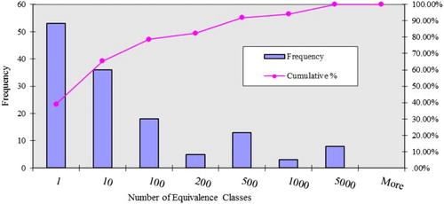
The 136 equivalence classes generated are based on the reflexive, symmetric and transitive relations of an object with respect to the subset of attributes. Of the 136 classes, 53 classes have cardinalities equal to unity and fewer than 124 classes have cardinalities less than 450. Figure 3 illustrates the frequency and cumulative distribution of equivalence classes. The distribution of the frequency of the number of equivalence classes shows a typical skewed characteristic. The larger concentration of objects in a single equivalence class indicates spatial homogeneity or ‘natural clustering’ of pixels with respect to attributes. In this respect, it would be interesting to see how the equivalence classes relate with the land cover classes. The subsequent section describes the approximate mapping of the land cover classes with the equivalence classes.

Figure 3. Frequency and cumulative distribution of equivalence classes.

3.4. Approximation evaluation by variable precision measures

Of all the decision classes (or more precisely, land cover classes), class ‘a’ shows a higher value of total cardinality and the larger number of equivalence classes in the lower approximation. There are 47 equivalence classes in the boundary region of class ‘a’. It means that there is uncertainty in assigning a single class ‘a’ to the objects belonging to these equivalence classes. The set approximation can further be evaluated by varying degrees of precision β. The approximation of the decision classes with respect to the given attribute set for a precision level of β = 0.0 indicates a low level of accuracy for class ‘a’, ‘b’ and ‘d’ (0.014, 0.065 and 0.045, respectively). This could be explained by the large cardinality of associated boundary region with these classes. The accuracy and specificity of class ‘c’ show the highest score for β = 0.0, which can also be explained by lower boundary region of the class. The prevalence of the large size of the boundary region indicates a higher level of uncertainty in the characterization process. As can be noticed from Table 6, by increasing the precision level β, the boundary region can be sliced down to a reasonable limit, thereby improving the measure of sensitivity, specificity and accuracy. For example, by decreasing the size of the boundary region in class ‘a’ from 47 to 0, the sensitivity and accuracy scores are improved from 0.0174 to 0.99 and 0.014407 to 0.7464, respectively. However, the sensitivity score for the remaining classes does not tend to improve with the thinning of boundary region. For classes ‘b’, ‘c’, ‘d’ and ‘e’, the effect of thinning is more significant in improving the specificity and accuracy score than the sensitivity score. This is because decreasing the boundary region does not necessarily increase the cardinality of lower approximation, which actually reflects the sensitivity measure.

Table 6. Approximation evaluations of land cover classes with variable precision level.

	Precision β = 0.0	Precision β = 0.25	Precision β = 0.5
Decision class: a
Sensitivity	0.017446	0.53588	0.99
Specificity	0.006157	0.05591	0.085061
Accuracy	0.014407	0.40669	0.7464
Decision class: b
Sensitivity	0.002059	0.002059	0.002059
Specificity	0.069213	0.992507	1.0
Accuracy	0.0648	0.927422	0.934422
Decision class: c
Sensitivity	0.004975	0.004975	0.004975
Specificity	0.563592	1.0	1.0
Accuracy	0.559794	0.993236	0.993236
Decision class: d
Sensitivity	0.009329	0.100605	0.102622
Specificity	0.051558	0.77568	0.9956
Accuracy	0.045894	0.685133	0.875744
Decision class: e
Sensitivity	0.001622	0.001622	0.001622
Specificity	0.307767	1.0	1.0
Accuracy	0.288623	0.937568	0.937569

Variable precision approximation provides flexible measures; however, often the relaxed precision requirements may not be desirable in subsequent model input. The trade-offs between the expected approximation performance and the precision level need to be compromised. Therefore, the varying degree of precision level needs standards for the evaluation of approximation parameters, which would render different set of approximations comparable.

3.5. Rule induction and prediction

In a rough set, reducts represent the most informative attribute. This involves formation of a discernibility matrix of the information where each tuple in table represents discrete two-dimensional spatial references. The prime implicants of the discernibility function provide the minimal subsets of attributes or reducts. The reducts are then used to generate decision rules from the decision table to generate basic minimal covering rules or a minimal number of possibly smallest rules covering all the cases. We used a rough set algorithm for inducing rule-based classification algorithm MODLEM (Stefanowski 1998; Stefanowski 2007; Stefanowski and Wilk 2007) classifiers. The classification strategy involves using nearest rules and class approximation. The class conditional entropy measure is used to choose the elementary ‘best’ condition of rule (i.e. the first candidate for the condition part). It heuristically generates unordered minimal set of rules for every land cover class (or its rough approximation in case of inconsistent examples) using a sequential covering scheme. The algorithm also allows the generation of certain rules from lower approximation and possible rules from the upper approximation of a rough set. In a land cover map of the real world, it is highly likely that in given sampling frame, the classes may not have equal representation in the model. To account for class imbalance (i.e. a small number of instances of minority classes), we used the Synthetic Minority Over-sampling Technique (SMOTE) (Chawla et al. 2002) algorithm. SMOTE generates random synthetic instances of the representative minority classes. The nearest neighbor method was used to artificially generate new representative samples. The rule induction algorithm generated a total of 2182 rules from the training set. It implies that the rough set rule induction was capable of compressing 78.44% of the training samples into decision rules. Finally, the induced rules are applied to testing instances to predict land cover classes by considering the strength of all completely matching rules. For a given training instance, if no rule fits the antecedent, the partial match is used to predict. Figure 4(a) shows the predicted land cover classes (with 79.74% correctly classified) and the misclassified pixels (Figure 4(b)).

Figure 4. (a) Land cover class prediction using a rough set rule induction method and (b) misclassified pixels.

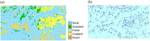
The distribution of misclassified pixels shows a trend of spatial clustering. The statistical significance of the spatial autocorrelation of the misclassified pixels can be tested by estimating the spatial autocorrelation coefficient by a Monte Carlo simulation. The calculated statistic of autocorrelation from the original mapped data can be compared with the n independently generated permutated statistics via randomization or bootstrap method. Davison and Hinkley (1997) provide a formula to determine the Monte Carlo p-values of the observed autocorrelation. A joint count statistic of misclassified pixels shows that the spatial autocorrelation is significant (at α = 0.05) with a p-value of .01 in a one-tailed test. The kappa coefficient (0.49) indicates a robust model performance against chance agreement. The weighted average producer and user accuracy is 78.5% and 80.4%, respectively. Since producer accuracy measures the degree of goodness of classification in a certain area, it fundamentally reflects the effect of omission error (Type I error), which measure the proportion of real-world feature not classified by the map. Similarly, the user accuracy can be used to estimate the commission error (or Type II error), that is, error introduced by assigning classes.

3.6. Comparing predictive performance

Cross-validations were performed to evaluate the quality of learned rough set model and to estimate the accuracy statistics. The result was compared with a baseline machine learning algorithm such as decision tree (C4.5) – an extension of ID3, a multilayered artificial neural network with one hidden layer also called multilayered perceptron (NN-MLP), SVM that uses LibSVM wrapper class and the popular naïve Bayes model. A confusion matrix was generated from the training and testing to evaluate the predictive performance.

The overall accuracy of the rough set rule induction method was found to be 79.74%, which is higher than neural network (NN-MLP) and decision tree and naïve Bayes and SVM (see Table 7). It reflects the model’s overall strong predictive capability. The high score of the overall classification accuracy of the model represents the global level accuracy in predicting the overall classes. In a confusion matrix, the diagonal element represents the count of correctly classified pixels. The overall accuracy indicates the percentage of the sum of correctly classified pixels. The kappa coefficient is a robust measure which indicates a model’s predictive performance beyond random assignment of class labels. The rough set model scored the highest kappa coefficient indicating the robustness of the model against chance agreement. The recall measure of a class indicates the true positive rate or sensitivity of that class, while precision or positive predictive value is a measure of the ratio of true positive and sum of true positive and false positive. The precision and recall measures reported in Table 7 are the weighted average of all the classes. Clearly, the precision and recall measures are highest in a rough set model than any other model which indicates a strong model sensitivity and positive predictive performance. The F-measure combines precision and recall by computing the harmonic mean of both of them. The F-measure of a rough set is clearly higher than those of NN-MLP, SVM, naïve Bayes and C4.5. Although the rough set outperforms other models, it appears that the overall model performance indicators of rough set and C 4.5 are relatively close.

Table 7. The comparison of overall predictive performances.

	Rough set rule induction (MODLEM)	Multi-layer neural network (NN-MLP)	Decision tree (C4.5)	Support vector machine (SVM) (LibSVM)	Naïve Bayes
Overall accuracy	79.74%	76.41%	79.40%	72.87%	67.26%
Kappa coefficient	0.49	0.33	0.44	0.027	0.26
Precision (producer accuracy)	0.785	0.65	0.77	0.66	0.67
Recall (user accuracy)	0.804	0.76	0.79	0.72	0.67
F-Measure	0.781	0.70	0.76	0.62	0.67

Finally, paired t-tests were performed to compare whether the difference between the predictive performance indicators (i.e. percent correct, kappa, F-measure) of the rough set model and that others models are statistically significant. It was found that at the .05 significance level, the differences among the predictive performance indicators of the rough set model and that of NN-MLP, SVM and naïve Bayes are statistically significant, that is, the rough set model outperforms NN-MLP and naïve Bayes. However, the difference between the rough set and the decision tree was not found statistically significant. Despite comparable performance with the decision tree, the computational cost of rough set rule induction could be potentially higher. As the algorithm sequentially generates rules from the positive examples of a given land cover class by discriminating all the negative examples, the decision boundaries in such cases are more complex and therefore the computational complexity may increase when the number of instances increases.

4. Conclusion

In this paper, we present an approach to discover knowledge under uncertainty for land cover classification and prediction. The variable precision approximation provides flexible measures for model performances by including relaxed precision requirements. The trade-offs between the expected approximation performance and the precision level need to be compromised. Therefore, the varying degree of precision level needs standards for evaluation of approximation parameters, which would render different sets of approximations comparable. The comparison of predictive performance shows that rough set rule induction performance scores are slightly higher than those of a baseline decision tree. However, the rough set rule induction method clearly outperforms the neural network (NN-MLP), SVM and naïve Bayesian in terms of all predictive indicators. The differences have been found statistically significant. The higher performance is attributable to the fact that rough set rules are derived based on the context of nearest neighbors as well as approximation space. Moreover, it offers improved semantics for handling imprecision in finite resolution spatial data. It helps identify the minimal subset of thematic layers (i.e. reducts in rough set) to preserve the spatial data integrity without any loss consistency. Additionally, the rough set-based knowledge discovery method could add significant advantage when data exhibit granular or natural clustering, particularly in remote sensing where pixels are spatially clustered. Unlike the neural network model which is essentially a black box model, the proposed approach preserves the underlying data semantics and does not assume any a priori statistical distribution of the data set. In particular, when the data are high dimensional (e.g. in hyperspectral image processing), the concept of reduct may prove to be useful in dimension reduction as well as image fusion. Additionally, the rough set and variable precision rough set formalism do not assume any distribution function or statistical inference and are transparent enough to interpret the outcome from the domain knowledge. Unlike the classical approach where there is the rigorous requirement of classification parameters and conditionings attributes thereby offering limited flexibility to incorporate imprecise or ambiguous evidences for representation of intrinsic uncertainty in data sets, the rough set approach provides flexibility and objective approximation schemes. However, the computational cost should be taken into account because the computation of reducts and rule induction from complex decision boundary may increase with the increase of data instances that needs to be addressed in future research.

Disclosure statement

No potential conflict of interest was reported by the author.

References

- Aggarwal, C. Charu. 2015. “Mining Spatial Data.” In Data Mining: The Textbook, 531–555. Cham: Springer.
- Albanese, A., S. Pal, and A Petrosino. 2012. “Rough Sets, Kernel Set and Spatio-Temporal Outlier Detection.” IEEE Transactions on Knowledge and Data Engineering (99): 1. doi:10.1109/tkde.2012.234.
- Allard, Denis. 2013. “J.-P. Chilès, P. Delfiner: Geostatistics: Modeling Spatial Uncertainty.” Mathematical Geosciences 45 (3): 377–380.
- Amarsaikhan, D., M. Saandar, M. Ganzorig, H. H. Blotevogel, E. Egshiglen, R. Gantuyal, B. Nergui, and D. Enkhjargal. 2012. “Comparison of Multisource Image Fusion Methods and Land Cover Classification.” International Journal of Remote Sensing 33 (8): 2532–2550.
- Atkinson, Peter M. 2001. “Geostatistical Regularization in Remote Sensing.” In Modelling Scale in Geographical Information Science, edited by N. Tate and P. M. Atkinson, 237–260. Chichester: John Wiley and Sons.
- Bae, Changseok, Wei-Chang Yeh, Yuk Ying Chung, and Sin-Long Liu. 2010. “Feature Selection with Intelligent Dynamic Swarm and Rough set.” Expert Systems with Applications 37 (10): 7026–7032.
- Banerjee, Sudipto, Bradley P. Carlin, and Alan E. Gelfand. 2014. Hierarchical Modeling and Analysis for Spatial Data. Boca Raton, FL: CRC Press.
- Beaubouef, Theresa, and Frederick E. Petry. 2010. Fuzzy and Rough Set Approaches for Uncertainty in Spatial Data. In Methods for Handling Imperfect Spatial Information, edited by Robert Jeansoulin, Odile Papini, Henri Prade, and Steven Schockaert, 1–11. Berlin, Heidelberg: Springer-Verlag.
- Beaubouef, Theresa, and Frederick Petry. 2013. “Uncertainty in Concept Hierarchies for Generalization in Data Mining.” In Efficiency and Scalability Methods for Computational Intellect, edited by Boris Igelnik and Jacek M. Zurada, 55–74. Hershey, PA: IGI Global.
- Brown, Daniel G., Robert Walker, Steven Manson, and Karen Seto. 2004. “Modeling Land use and Land Cover Change.” In Land Change Science: Observing, Monitoring, and Understanding Trajectories of Change on the Earth's Surface, edited by G. Gutman, A. Janetos, C. Justice, E. Moran, J. Mustard, R. Rindfuss, D. Skole, and B. L. Turner II, 395–409. Dordrecht: Kluwer Academic Publishers.
- Brus, Jan, and Vilém Pechanec. 2015. “The User Centered Framework for Visualization of Spatial Data Quality.” In Modern Trends in Cartography, edited by Jan Brus, Alena Vondrakova, and Vit Vozenilek, 325–338. Cham: Springer.
- Chawla, Nitesh V., Kevin W. Bowyer, Lawrence O. Hall, and W. Philip Kegelmeyer. 2002. “SMOTE: Synthetic Minority Over-Sampling Technique.” Journal of Artificial Intelligence Research, 16: 321–357.
- Davison, Anthony Christopher, and David Victor Hinkley. 1997. Bootstrap Methods and Their Application, Vol. 1. Cambridge, NY: Cambridge University Press.
- Ding, Weiping, Jiandong Wang, and Zhijin Guan. 2012. “Cooperative Extended Rough Attribute Reduction Algorithm Based on Improved PSO.” Journal of Systems Engineering and Electronics 23 (1): 160–166.
- Düntsch, I., and G. Gediga. 1998. “Uncertainty Measures of Rough set Prediction.” Artificial Intelligence 106 (1): 109–137.
- Evans, Tom P., and Emilio F. Moran. 2002. “Spatial Integration of Social and Biophysical Factors Related to Landcover Change.” Population and Development Review 28: 165–186.
- Fayyad, U. M., and K. B. Irani. 1993. “Multi-interval Discretization of Continuous-Valued Attributes for Classification Learning.” Artificial Intelligence 13: 1022–1027.
- Feng, Yongjiu, and Yan Liu. 2015. “Fractal Dimension as an Indicator for Quantifying the Effects of Changing Spatial Scales on Landscape Metrics.” Ecological Indicators 53: 18–27.
- Gamba, Paolo. 2014. “Image and Data Fusion in Remote Sensing of Urban Areas: Status Issues and Research Trends.” International Journal of Image and Data Fusion 5 (1): 2–12. doi:10.1080/19479832.2013.848477.
- Gao, Zhenji, Lun, Wu, and Yong Gao. 2007. “Topological Relations Between Vague Objects in Discrete Space Based on Rough Model.” In Fuzzy Information and Engineering, edited by Bing-Yuan Ca, 852–861. Berlin, Heidelberg: Springer.
- Ge, Yong, Feng Cao, Yunyan Du, V. Chris Lakhan, Yingjie Wang, and Deyu Li. 2011. “Application of Rough set-Based Analysis to Extract Spatial Relationship Indicator Rules: An Example of Land use in Pearl River Delta.” Journal of Geographical Sciences 21 (1): 101–117. doi:10.1007/s11442-011-0832-y.
- Ge, Y., F. Cao, and R. F. Duan. 2011. “Impact of Discretization Methods on the Rough set-Based Classification of Remotely Sensed Images.” International Journal of Digital Earth 4 (4): 330–346. doi:10.1080/17538947.2010.494738.
- Griffith, Daniel A., David W. Wong, and Yongwan Chun. 2016. “Uncertainty-Related Research Issues in Spatial Analysis.” Uncertainty Modelling and Quality Control for Spatial Data, edited by W. Shi, B. Wu, and A. Stein, 1. Boca Raton: CRC Press.
- Grünwald, Peter D. 2007. The Minimum Description Length Principle. London: MIT Press.
- Guptill, Stephen C., and Joel L. Morrison. 1995. Elements of Spatial Data Quality. Oxford: Elsevier.
- Han, Jiawei, Micheline Kamber, and Jian Pei. 2012. Data Mining: Concepts and Techniques: Concepts and Techniques. New York: Elsevier.
- Harvey, Francis, and Yee Leung. 2015. Advances in Spatial Data Handling and Analysis. Cham: Springer International Publishing.
- Hong, T., K. Hart, L.-K. Soh, and Ashok Samal. 2014. “Using Spatial Data Support for Reducing Uncertainty in Geospatial Applications.” GeoInformatica 18 (1): 63–92.
- Huang, Kuang Yu. 2012. “An Enhanced Classification Method Comprising a Genetic Algorithm, Rough Set Theory and a Modified PBMF-Index Function.” Applied Soft Computing 12 (1): 46–63.
- Hunsaker, Carolyn T., Michael F. Goodchild, Mark A. Friedl, and Ted J. Case. 2013. Spatial Uncertainty in Ecology: Implications for Remote Sensing and GIS Applications. New York: Springer.
- Jiang, Bin, and S. Anders Brandt. 2015. A Fractal Perspective on Scale in Geography. arXiv preprint arXiv:1509.08419.
- Kinkeldey, Christoph. 2014. “A Concept for Uncertainty-Aware Analysis of Land Cover Change Using Geovisual Analytics.” ISPRS International Journal of Geo-Information 3 (3): 1122–1138.
- Komorowski, Jan, and Aleksander Øhrn. 1999. “Modelling Prognostic Power of Cardiac Tests Using Rough Sets.” Artificial Intelligence in Medicine 15: 167–191.
- Lechner, Alex M., William T. Langford, Sarah A. Bekessy, and Simon D. Jones. 2012. “Are Landscape Ecologists Addressing Uncertainty in Their Remote Sensing Data?” Landscape Ecology 27 (9): 1249–1261.
- Lei, T. C., S. Wan, and T. Y. Chou. 2008. “The Comparison of PCA and Discrete Rough Set for Feature Extraction of Remote Sensing Image Classification – A Case Study on Rice Classification, Taiwan.” Computational Geosciences 12 (1): 1–14.
- Leung, Yee, Tung Fung, Ju-Sheng Mi, and Wei-Zhi Wu. 2007. “A Rough set Approach to the Discovery of Classification Rules in Spatial Data.” International Journal of Geographical Information Science 21 (9): 1033–1058.
- Li, Jinhai, Changlin Mei, and Yuejin Lv. 2011. “A Heuristic Knowledge-Reduction Method for Decision Formal Contexts.” Computers & Mathematics with Applications 61 (4): 1096–1106.
- Lin, Jie, Robert G. Cromley, Daniel L. Civco, Dean M. Hanink, and Chuanrong Zhang. 2013. “Evaluating the Use of Publicly Available Remotely Sensed Land Cover Data for Areal Interpolation.” GIScience & Remote Sensing 50 (2): 212–230. doi:10.1080/15481603.2013.795304.
- Loveland, T. R., B. C. Reed, J. F. Brown, D. O. Ohlen, Z. Zhu, L. W. M. J. Yang, and J. W. Merchant. 2000. “Development of A Global Land Cover Characteristics Database and IGBP DISCover from 1 km AVHRR Data.” International Journal of Remote Sensing 21 (6–7): 1303–1330.
- Malczewski, Jacek. 2006. “GIS-Based Multicriteria Decision Analysis: A Survey of the Literature.” International Journal of Geographical Information Science 20 (7): 703–726.
- Masek, Jeffrey G., Daniel J. Hayes, M. Joseph Hughes, Sean P. Healey, and David P. Turner. 2015. “The Role of Remote Sensing in Process-Scaling Studies of Managed Forest Ecosystems.” Forest Ecology and Management 355: 109–123.
- Mi, Ju-Sheng, Wei-Zhi Wu, and Wen-Xiu Zhang. 2004. “Approaches to Knowledge Reduction Based on Variable Precision Rough set Model.” Information sciences 159 (3): 255–272.
- Miller, Harvey J., and Jiawei Han. 2009. Geographic Data Mining and Knowledge Discovery. Boca Raton: CRC Press.
- Morris, Ashley, Piotr Jankowski, Brian S. Bourgeois, and Frederick E Petry. 2010. “Decision Support Classification of Geospatial and Regular Objects Using Rough and Fuzzy Sets.” In Uncertainty Approaches for Spatial Data Modeling and Processing: A Decision Support Perspective, edited by J. Kacprzyk, F. E. Petry, and A. Yazici, 3–8. Berlin, Heidelberg: Springer.
- Pan, Xin, Shuqing Zhang, Huaiqing Zhang, Xiaodong Na, and Xiaofeng Li. 2010. “A Variable Precision Rough set Approach to the Remote Sensing Land use/Cover Classification.” Computers & Geosciences 36 (12): 1466–1473.
- Patra, Swarnajyoti, Prahlad Modi, and Lorenzo Bruzzone. 2015. “Hyperspectral Band Selection Based on Rough set.” IEEE Transactions on Geoscience and Remote Sensing 53 (10): 5495–5503.
- Pawlak, Zdzisław. 2002. “Rough Sets and Intelligent Data Analysis.” Information Sciences 147 (1): 1–12.
- Pawlak, Zdzisław, and Andrzej Skowron. 2007. “Rudiments of Rough Sets.” Information Sciences 177 (1): 3–27.
- Perez, Liliana, Trisalyn Nelson, Nicholas C. Coops, Fabio Fontana, and C. Ronnie Drever. 2016. “Characterization of Spatial Relationships Between Three Remotely Sensed Indirect Indicators of Biodiversity and Climate: A 21years’ Data Series Review Across the Canadian Boreal Forest.” International Journal of Digital Earth, 1–21. doi:10.1080/17538947.2015.1116623.
- Petry, Frederick, and Paul Elmore. 2015. “Geospatial Uncertainty Representation: Fuzzy and Rough Set Approaches.” In Fifty Years of Fuzzy Logic and its Applications, 483–497. Cham: Springer International Publishing.
- Pogson, Mark, and Pete Smith. 2015. “Effect of Spatial Data Resolution on Uncertainty.” Environmental Modelling & Software 63: 87–96.
- Riccio, Daniele, and Giuseppe Ruello. 2015. “Synthesis of Fractal Surfaces for Remote-Sensing Applications.” IEEE Transactions on Geoscience and Remote Sensing 53 (7): 3803–3814.
- Robertson, Colin, Jed A. Long, Farouk S. Nathoo, Trisalyn A. Nelson, and Cameron C. F. Plouffe. 2014. “Assessing Quality of Spatial Models Using the Structural Similarity Index and Posterior Predictive Checks.” Geographical Analysis 46 (1): 53–74.
- Sarkar, Bikash Kanti, Shib Sankar Sana, and Kripasindhu Chaudhuri. 2012. “A Genetic Algorithm-Based Rule Extraction System.” Applied Soft Computing 12 (1): 238–254.
- Serra, Pere, Xavier Pons, and David Saurí. 2008. “Land-cover and Land-use Change in A Mediterranean Landscape: A Spatial Analysis of Driving Forces Integrating Biophysical and Human Factors.” Applied Geography 28 (3): 189–209.
- Shekhar, Shashi, James Kang, and Vijay Gandhi. 2009. “Spatial Data Mining.” In Encyclopedia of Database Systems, edited by L. Liu and M. T. Zsu, 2695–2698. New York: Springer.
- Sheppard, Eric, and Robert B. McMaster. 2008. Scale and Geographic Inquiry: Nature, Society, and Method. Malden, MA: Wiley.
- Sikder, I. 2008. “Modeling Predictive Uncertainty in Spatial Data.” In Handbook of Research on Geoinformatics, edited by H. A. Karimi, 1–5. Dhaka: Information Science Reference.
- Sikder, I. 2010, January 9–10. “Rough Set Theory and Decision Analysis.” Paper presented at the International Conference on Industrial Engineering and Operations Management (IEOM) Dhaka, Bangladesh.
- Sikder, Iftikhar U., and Toshinori Munakata. 2009. “Application of Rough set and Decision Tree for Characterization of Premonitory Factors of low Seismic Activity.” Expert Systems with Applications 36 (1): 102–110.
- Song, Xiao-Peng, Chengquan Huang, Min Feng, Joseph O. Sexton, Saurabh Channan, and John R. Townshend. 2014. “Integrating Global Land Cover Products for Improved Forest Cover Characterization: an Application in North America.” International Journal of Digital Earth 7 (9): 709–724. doi:10.1080/17538947.2013.856959.
- Stefanowski, J. 1998. “The rough set based rule induction technique for classification problems.” Paper presented at the Proceedings of 6th European Conference on Intelligent Techniques and Soft Computing EUFIT, Aachen.
- Stefanowski, Jerzy. 2007. “On Combined Classifiers, Rule Induction and Rough Sets.” In Transactions on Rough Sets VI, 329–350. Warsaw: Springer.
- Stefanowski, Jerzy, and Szymon Wilk. 2007. “Improving Rule Based Classifiers Induced by MODLEM by Selective Pre-Processing of Imbalanced Data.” Paper presented at the Proceedings of the RSKD Workshop at ECML/PKDD, Warsaw.
- Straume, Kjersti. 2014. “The Social Construction of a Land Cover map and its Implications for Geographical Information Systems (GIS) as a Management Tool.” Land Use Policy 39: 44–53.
- Thackway, Richard, Leo Lymburner, and Juan Pablo Guerschman. 2013. “Dynamic Land Cover Information: Bridging the gap Between Remote Sensing and Natural Resource Management.” Ecology and Society 18 (1): 2.
- Trabelsi, Salsabil, Zied Elouedi, and Pawan Lingras. 2011. “Classification with Dynamic Reducts and Belief Functions.” In Transactions on Rough Sets XIV, 202–233. Berlin, Heidelberg: Springer.
- Turner, Monica G., Robert V. O’Neill, Robert H. Gardner, and Bruce T. Milne. 1989. “Effects of Changing Spatial Scale on the Analysis of Landscape Pattern.” Landscape Ecology 3 (3–4): 153–162.
- Vinh, Nam Nguyen, and Bac Le. 2012. “Incremental Spatial Clustering in Data Mining Using Genetic Algorithm and R-Tree.” In Simulated Evolution and Learning, 270–279. Berlin, Heidelberg: Springer.
- Wang, Qunming, Wenzhong Shi, Peter M Atkinson, and Eulogio Pardo-Igúzquiza. 2016. “A New Geostatistical Solution to Remote Sensing Image Downscaling.” IEEE Transactions on Geoscience and Remote Sensing 54 (1): 386–396.
- Weng, Qihao. 2014. Scale Issues in Remote Sensing. Hoboken, NJ: Wiley.
- Wu, Hua, and Zhao-Liang Li. 2009. “Scale Issues in Remote Sensing: A Review on Analysis, Processing and Modeling.” Sensors 9 (3): 1768–1793.
- Xie, Feng, Yi Lin, and Wenwei Ren. 2011. “Optimizing Model for Land use/Land Cover Retrieval From Remote Sensing Imagery Based on Variable Precision Rough Sets.” Ecological Modelling 222 (2): 232–240. doi:10.1016/j.ecolmodel.2010.08.011.
- Xu, Yitian, Laisheng Wang, and Ruiyan Zhang. 2011. “A Dynamic Attribute Reduction Algorithm Based on 0–1 Integer Programming.” Knowledge-Based Systems 24 (8): 1341–1347.
- Yang, Xibei, Yunsong Qi, Xiaoning Song, and Jingyu Yang. 2013. “Test Cost Sensitive Multigranulation Rough set: Model and Minimal Cost Selection.” Information Sciences 250: 184–199.
- Yun, Ouyang, and Jianwen Ma. 2006. “Land Cover Classification Based on Tolerant Rough set.” International Journal of Remote Sensing 27 (14): 3041–3047.
- Zandbergen, P. A., T. C. Hart, K. E. Lenzer, and M. E. Camponovo. 2012. “Error Propagation Models to Examine the Effects of Geocoding Quality on Spatial Analysis of Individual-Level Datasets.” Spatial and spatio-temporal epidemiology 3 (1): 69–82.
- Zhang, Jixian. 2010. “Multi-source Remote Sensing Data Fusion: Status and Trends.” International Journal of Image and Data Fusion 1 (1): 5–24. doi:10.1080/19479830903561035.
- Zhao, Jian, and Xin Pan. 2015. “Remote Sensing Image Feature Selection Based on Rough Set Theory and Multi-Agent System.” Paper presented at the 12th International Conference on Fuzzy Systems and Knowledge Discovery (FSKD), 2015.
- Ziarko, Wojciech P. 2012. Rough Sets, Fuzzy Sets and Knowledge Discovery: Proceedings of the International Workshop on Rough Sets and Knowledge Discovery (RSKD’93), Banff, Alberta, Canada, 12–15 October 1993: Springer Science & Business Media.