Monitoring the built-up environment of Shanghai on the street-block level using SAR and volunteered geographic information

ABSTRACT

In this geo-statistical analysis of change detection, we illustrate the evolution of the built-up environment in Shanghai at the street-block level. Based on two TerraSAR-X image stacks with 36 and 15 images, covering the city centre of Shanghai for the time period from 2008 to 2015, a set of coherence images was created using a small baseline approach. The road network from Open Street Map, a volunteered geographic information product, serves as the input dataset to create street-blocks. A street-block is surrounded by roads and resembles a ground parcel, a real estate property – a cadastral unit. The coherence information is aggregated to these street-blocks for each observation and the variation is analysed over time. An analysis of spatial autocorrelation reveals clusters of similar behaviours. The result is a detailed map of Shanghai highlighting areas of change. We argue that the aggregation and grouping of synthetic aperture radar coherence image information to real-world entities (street-blocks) is comprehensible and relevant to the urban planning process. Therefore, this research is a contribution to the community of urban planners, designers, and government agencies who want to monitor the development of the urban landscape.

KEYWORDS:

• SAR
• change detection
• urban area
• volunteered geographic information

1. Introduction

Shanghai is the largest city in China with over 24 million inhabitants, but the entire metropolitan area is estimated to even have residents, around 34 million people (OECD 2015). Since the opening and reform in China, but especially since the 1990s, Shanghai has undergone a rapid increase in population from around 13 million in 1990 to approximately 23 million in 2010. The inflow of around 10 million people over just 20 years has led to a tremendous increase in the size and the density of the urban area.

Considering such fast growth rates, close monitoring of urbanization is crucial to ensure sufficient infrastructural development as well as to guarantee the safety and security of buildings and development while suppressing illegal building activities. Considering the sheer size of the city, this is not an easy task, but remote sensing offers a means for effective monitoring of urbanization in large, dynamic metropolitan areas such as Shanghai. Considering the speed of urbanization, update up-to-date information is elusive. synthetic aperture radar (SAR) fills this void, providing timely observations based on fast revisit rates, a good update speed and almost complete weather independency, SAR avoids seasonal observation gaps that can hinder optical observations in Shanghai.

SAR offers several possible approaches for urban area detection. Using polarimetric data, polarimetric signatures caused by double-bouncing reflections typically indicate the presence of urban settlement patterns. However, in the trade-off between spatial resolution to polarimetric image acquisition, data providers as well as end-users often go with the higher spatial resolution, making polarimetric images less accessible. Alternatively, high amplitudes indicate man-made objects and a proxy indicator of urban settlement areas, especially if clustered. Another widespread method of measuring urbanization is based on the interferometric coherence of the SAR data. Urban areas keep phase signals coherent over long periods, while vegetated areas lose coherence rapidly, depending on the type of vegetation, the wavelength of the SAR system, and the temporal distance between the acquisitions.

Although coherence delivers high-quality measurement of phase stability and therefore is a powerful indicator of man-made objects, nevertheless a single resolution cell with high coherence is by itself not a meaningful indicator of urbanity. Only the appearance of several resolution cells showing high coherence in a spatial cluster can be considered a reliable indicator. Typically, this is guaranteed by filtering the image; for example, by down-sampling the coherence image or by morphological operators.

A more effective approach, however, groups pixels by natural and meaningful features. In our approach, we use volunteered geographic information (VGI) to group the pixels to meaningful entities and then use spatial autocorrelation measures for spatio-temporal analysis of dynamic urbanization processes. VGI allow the creation and sharing of spatial data, making possible the production of user-generated geographical content (Goodchild 2007; Elwood 2008; Elwood, Goodchild, and Sui 2012). Everyday user-creators bypass traditional producers of geographic knowledge such as government agencies or commercial enterprises and create resources such as Open Street Map (OSM) that reflect local knowledge of specific areas. Lacking clearly defined authorship, these data come as is, and must be treated carefully as it might be of questionable quality and credibility (Brown et al. 2013).

Despite these limitations, OSM provides timely and perhaps the only publically available detailed street network information for Shanghai. Vector GIS data are not readily available from official sources and what is available is often out of date and at too coarse a scale for meaningful analysis. We therefore used OSM data to generate street-block area units, aggregated coherence information to these street-blocks for each observation, and analysed the variation over time. The urban dynamics of Shanghai become transparent and understandable when the rich spatial–temporal information from SAR imagery is combined with street-blocks derived from OSM, filling a gap in our understanding of this changing metropolis.

The presented study has to be viewed from the perspective of data availability in China. Often official datasets are not easily accessible due to the socio-political circumstances, and alternative data sources have to be consulted. Also, foreigners are not allowed to collect geo-spatial data themselves (Hvistendahl 2013).

In the next section, we will describe the test site and the data used for our experiment. In Section 3, we will describe the methods used in detail and then present and discuss our results. Finally, conclusions are drawn.

2. Data and test site description

Shanghai is a fast growing metropolitan area of global importance. Monitoring and understanding Shanghai’s urbanization process is crucial for predicting the future development of Shanghai that can give us insights into the overall urbanization process in China.

For our experiments in Shanghai, we processed two TerraSAR-X stripmap image stacks with 36 and 15 images. Both image stacks are acquired in vertical vertical (VV) polarization, at a wavelength of around 3.1 cm, and from descending orbits. The differences between the stacks are the time of recording (first stack covers the time period from April 2008 to October 2012 and the second from April 2013 to May 2015), and the spatial coverage. The second stack is slightly shifted to the south of Shanghai, but still covers the city centre. The incidence angle of the first stack is ∼24°, while the second stack is taken at 42°. The coherence results are two time-series image stacks.

A set of 51 SAR images leads to a high temporal resolution, which allows us to pinpoint urban change on the structural level (buildings and infrastructure) very accurately, for example, the destruction of a street-block. However, a reduced number of images would be sufficient for the observation of urban developments as well. In our case, the dataset was available to us and demonstrates that SAR is capable of acquiring images stacks on demand, with high temporal resolution, ignoring (most) weather conditions. An optical system would have a significant drawback in that regard.

A survey (at http://landsatlook.usgs.gov) of available optical image data from Landsat 7 ETM (SLC off) between 2010 and 2015 revealed 12 images over the city centre of Shanghai with 0% cloud coverage, and 20 images when accepting a cloud coverage 10%. Landsat 8 OLI delivered one image without cloud coverage and 22 with 10%. Consistently getting images is an advantage of microwave remote sensing.

This consistency allows us to generate stacks of coherence images to perform a coherence change detection (CCD) analysis. A CCD to identify stable objects and changes, especially over urban areas, is a validated and proven method in microwave remote sensing. In Esch et al. (2012, 2013), Taubenböck and Wiesner (2015), and Taubenböck et al. (2012), the authors show how SAR data are used to derive a global map of urban settlements using coherence imagery from the TanDEM-X mission.

To derive street-blocks, we used VGI data from OSM (2014). On this platform, users create and control the content of spatial data themselves and anybody can contribute. OSM is globally available, but the accuracy and completeness depends on the local user activity and the quality can vary widely. In Zhou, Huang, and Jang (2014) and mainly in Zheng and Zheng (2014), the authors have assessed the completeness and positional accuracy of OSM data in China by comparing it to Baidu Map data and the Chinese Statistical Yearbook (both are not available to us). Their conclusion is that Shanghai, Beijing, Nanjing, and Hong Kong are ‘most complete’, while cities in western China are underdeveloped in OSM; however, the general trend is towards more contributions and increased completeness for entire China This makes OSM the most comprehensive and publically available dataset for Shanghai at this time.

3. Method

In our work, we combine SAR coherence data derived from small-baseline-like time-series data. SAR coherence is a measure of similarity between interferometric SAR scenes (see, e.g. Wang, Liao, and Perissin 2010). Temporal decorrelation caused by changes of the backscattering object over time is a major cause of coherence loss, making coherence a good measurement of local stability in the wavelength dimension of the SAR system.

Aggregating the pixels to street-blocks derived from VGI data guarantees the clustering of the coherence data into clusters with real-world meaning and importance, such as street-blocks. After the aggregation of coherence data to street-blocks, spatial autocorrelation analysis provides an empirical means to identify meaningful clusters of change in the built environment of the Shanghai central area.

3.1. SAR coherence time series from a small baseline approach

Coherence analysis is based on two TerraSAR-X stripmap data stacks. For each stack, the images are co-registered and resampled to a single master image. After co-registration and resampling, all possible combinations for the 36 and 15 images are calculated with regard to the temporal and perpendicular baseline information. If we consider all possible combinations, we have 630 for the first stack and 105 for the second stack. However, for our time-series analysis, it is not necessary to include all possible interferograms. Instead, we are forming interferograms that guarantee coherence and a sufficient coverage over time. We therefore follow a small-baseline approach and chose only those combinations that satisfy the criteria of a temporal baseline (B_temp) ≤90 days and a perpendicular baseline (B_perp) ≤150 m. These thresholds ensure a minimization of temporal and geometrical decorrelation and therefore avoid an unwanted loss in coherence estimation accuracy.

The resolution of the TerraSAR-X stripmap images is approximately 3 m, which is very detailed when analysing urban areas on a street-block level. For processing the data on a street-block level, this is not necessary and we therefore decrease the resolution by multi-looking the coherence image. Afterwards, we use an anisotropic diffusion (AD) filter, as it is used in medical imaging and suggested by Perona and Malik (1990) and Gerig et al. (1992), to reduce the speckle effect (Figure 1).

Figure 1. SAR coherence image filtered by AD (iterations = 5, K = 50 and Δ = 1/7) created from two TerraSAR-X strip map images (28 March and 9 April 2009), showing the northern part of the city centre.

3.2. Aggregating coherence into clusters

Spatial coherence is typically based on a window function where the quality of the estimation depends on the size of the window (see, e.g. Bamler and Hartl 1998). A larger window guarantees better coherence estimation, but this also reduces the spatial resolution of the estimated coherence.

The problem of this approach is that with large window sizes, the estimated coherence improves if the pixels in the window are homogenous; however, the larger the window, the less likely that it is homogenous. An effective coherence estimation includes a large number of homogenous pixels. Alternatively, adaptive window functions therefore are often better suited than a fixed window-based function. This is even more true for heterogeneous areas like the complex urban areas of Shanghai.

Our alternative, however, is the aggregation of pixels for the coherence estimation based on additional information. In our work, we follow this strategy by using street-blocks derived from OSM (see Section 3.3) as basis for our pixel aggregation. But, a street-block includes a large amount of heterogeneity and is by itself not a perfect basis for the coherence estimation. Therefore, we first estimate a coherence based on a small window of 5 × 5 pixels. These coherence estimations are then aggregated to the street-block level. In this way, the coherence estimations are aggregated to ‘natural’ (rather man-made) features with a clear ‘real-world’ meaning.

3.3. Retrieving street-blocks from OSM

On OSM, users create and control the content of spatial data themselves. Anybody can contribute roads, points of interests, and place names by uploading geographic data in the form of global positioning system (GPS) tracks or positions. OSM also allows users to classify roads into different categories. This can, and does, lead to inconsistencies in the road network classification. We therefore treat all road lines equally to form the street-blocks. An example is shown in Figure 2. Roads that cross each other will be converted to polygons; lines representing dead end roads or roads with an end that does not touch the boundary of another road will simply disappear.

Figure 2. An example of a street-block (marked in read, other roads in grey), without (left) and with (right) optical satellite image.

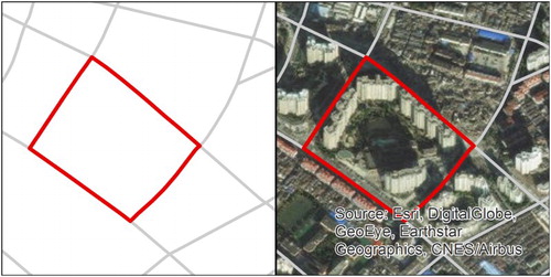
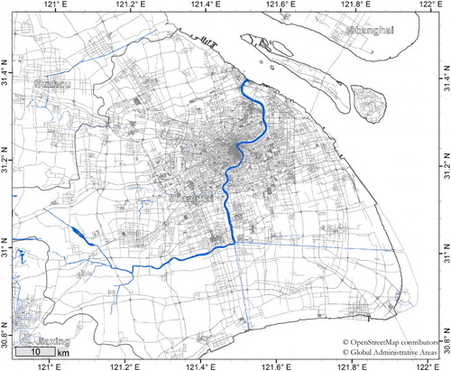
We selected roads and major rivers and canals as well as the administrative boundary of Shanghai according to Global Administrative Areas dataset (GADM) to create the street-blocks for the coherence data clustering. The road network as it appears on OSM with major rivers and the administrative boundary according to the GADM (Hijmans 2009) are illustrated in Figure 3.

Figure 3. Road network and major rivers in Shanghai according to OpenStreetMap (2014) and administrative boundaries from Hijmans (2009).

An area encircled by a road is an entity – a unit of measurement – in our approach. Roads can be dividers between different usages such as the contrast of a construction-side next to a park or shopping mall. Street-blocks also resemble visual elements or components in the urban landscape that are identifiable by the people that live within that space. Therefore, a street-block entity can be considered meaningful and with a clear real-world relation.

However, there are points that need to be considered. A unit may have multiple usages within and may develop differently over time in a single street-block. Also, OSM data are of varying quality and completeness. That may differ over the Shanghai metropolitan area, with probably a better quality in the centre where many people contribute to the data, but with probably less accurate information on the outskirts with lesser contributors. However, we have no reliable way of guaranteeing the overall consistency of the data over the test area.

3.4. Spatial autocorrelation of the coherence clusters

Spatial autocorrelation follows Tobler’s first law of geography (see Tobler 1970, 236): ‘everything is related to everything else, but near things are more related than distant things’. With spatial statistics that consider the value of each object, clusters of similar values can be identified. This procedure is also called local measurement of spatial autocorrelation (LISA) in the GeoDA (Anselin 2005; Anselin, Syabri, and Kho 2006) software package. Moran’s I value that is also produced during that procedure is a single value that gives evidence whether values of a spatial dataset are clustered or not. This value ranges between −1 and 1, where −1 refers to no clustering (totally dispersed values) and 1 refers to a high degree of clustering of similar values.

In this analysis, we are interested in the street-blocks that experienced change – expressed through the coherence value – over time. To find clusters of street-blocks (larger development projects), we use the standard deviation of the average coherence value of a street-block. Blocks of high variability (a high standard deviation) are probably undergoing changes in the built-up environment. LISA analysis allows us to detect these clusters.

4. Results and discussion

The results of the aggregation of coherence values to street-blocks is explained based on four figures and a time series of optical images that outline the results from basic visualization to individual street-blocks, the evolution of a street-block over time to clustering of street-blocks of high variability over the entire observation period.

4.1. Aggregated raster data to street-blocks

In Figure 4, the data from coherence images are represented in two ways. In Figure 4(a), the images are shown as raster data, the common way in remote sensing. The coherence images of both stacks are visualized with a red outline that depicts the footprints of the images. Only the overlapping area along the Huangpu river, running from the southwest to the northeast, is covered by both stacks. Figure 4(b) – after converting image pixels to vector points and aggregating them to street-blocks – shows a representation of average coherence values per parcel. As can be seen, the same area is covered, but split up and sectored by street-block units.

Figure 4. Raster representation of coherence images from stack 1 and 2 (a), and on the right side (b) the same data aggregated to street-blocks according to the road network.

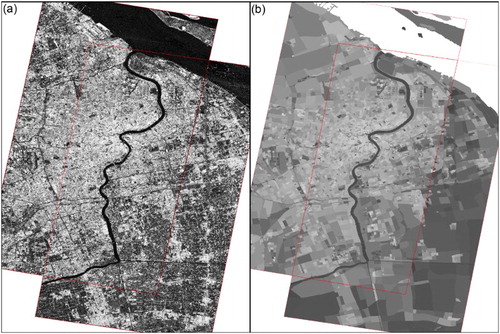
From Figure 4, we see the convoluted and noisy ‘salt-and-pepper’ effect of SAR coherence raster images collapsed into homogenous units that correspond to real-world entities/objects. An image filter on the other hand aggregates coherence based on its kernel and is not necessarily associated with a real-world entity that is identifiable on the ground – a street-block. The river – even though not a ‘street’ – is distinguishable and so are blocks within the city and around the city. A high contrast block can be recognized in comparison with its surrounding blocks. The assumption is that urban development happens on a block-by-block basis, and therefore the aggregation of coherence information to the street-block level is reasonable.

Going into more details, Figure 5 showcases three areas in the urban landscape of Shanghai. Each street-block in (a,c,e) represents its average coherence for one instance of a coherence observation. In the second row of Figure 5(b,d,f) is a corresponding subset of an optical image of the same area. In (a,b) a dense urban environment is depicted. The street-blocks in (a) show high coherence values, indicating a strong influence of man-made infrastructure and architecture. From the optical image (the actual date of this image is unknown), no indications of change are visible.

Figure 5. The representation of street-block coherence of three different areas within the urban area of Shanghai.

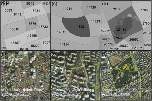
In group (c,d), the street-block with the ID 14302 shows a decreased coherence value compared to its surroundings. This indicates that change occurred between the acquisitions of the two SAR images. Evidence for this development is visible from (d) of the same figure. Six (completed) buildings can be identified in the same street-block and an area that appears to be still under development (brownish colour) is seen in the northeast section of the same street-block. Since the surrounding blocks do not show change in the coherence (their values are high), the assumption of change on a block-by-block basis is further solidified.

Change, however, is not necessarily caused by construction. The group (e,f) of Figure 5 illustrates the case of a city park. Here, the coherence values of street-blocks 27430 and 27636 are comparatively low due to the vegetation, and the lake within the park. The point that should be made is that a different usage of urban entities (parcels) and land-cover types can be inferred from the data.

4.2. Time series of coherence change

The detection of change and the variability of coherence over time are illustrated in Figure 6. This figure is divided into three columns with: (1) the standard deviation of the average coherence value over the observation time of the first image stack, where black indicates a strong variability and white a rather stable unchanging environment, (2) a representation of a filtered and resampled SAR coherence image as in Figure 1 or Figure 4(a), and (3) graphs that show the evolution of the coherence value over the entire observation time of both image stacks. Each scene has markings (green, red, and blue) for three nearby street-blocks of different standard deviation/variability values – a black (marked in green), a medium grey (red), and a white (blue), the same colour code is also used in the graphs.

Figure 6. Three groups of three different street-blocks are illustrated. Divided into three rows: the first column shows the standard deviation of the average coherence value of the first stack (black indicates high variability, white stability), the second column is a filtered and resampled coherence image of the same extent, and the third column is graphs showing the coherence values, for each of the street-blocks, for all coherence observations (the line is a linear interpolation).

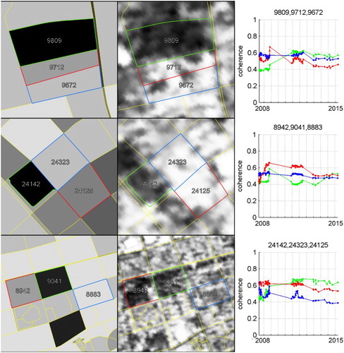
In the first row, parcel 9809 (green) is depicted in black, indicating high coherence variability and therefore change over time. The medium grey parcel, 9712 (red), should have less variability and 9672 (blue) is stable. This can be seen from the green graph that starts around a coherence value of 0.4 in 2008 before it increases to over 0.6 and then slightly decreases towards 2015. The red parcel (medium grey) is of a lower standard deviation, supported by the graphs. Even with the outliers in 2010, the coherence stays lower than 0.6 and higher than 0.4 throughout the observation time. The blue line in parcel 9672 is the most constant, only slightly diverging from a 0.6 coherence value and slightly dropping to around 0.5 during the acquisition time of the second stack. This development cannot be identified from the coherence image in the centre of the first row. External Google Earth optical imagery verifies this change.

The parcels in the second and third rows can be analysed in the same manner as the first row. Block 24142 (green) shows the highest variability, while 24125 (red) and 24323 (blue) experienced less change over time. The street-block represented in blue has a rather constant line with minimal variation, while the curves of the other two blocks are more unsteady. This time-series pattern reveals for each parcel, if it is experiencing development and/or change or not.

In the last row of Figure 6, block 9041 (green) shows a drastic change in coherence from 0.4 to over 0.6 in 2012 until the end of the observation in 2015. This means that the street-block has undergone development from barren land/vegetation to a built-up environment with man-made structures.

4.3. Clustering of high variability street-blocks

After establishing that change of coherence can be linked to street-blocks and the evolution can be followed over time, we can now uncover clusters of similar coherence behaviour. Figure 7 is the representation of spatial autocorrelation clusters, grouping the standard deviation of the coherence value. This LISA analysis gives clusters of similar standard deviation values per street-block, or variability (change). The calculated Moran’s I value for the standard deviation is at ∼0.5 that means that the data are clustered.

Figure 7. Clusters of similar coherence characteristics: red are clusters of high variability and blue are clusters of particularly low variability.

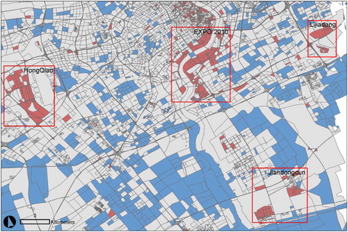
Focusing on the clusters of high variability; there are four main groups of street-blocks that show an increased standard deviation and that have faced changed in the built-up environment. To the west of the city centre is Hongqiao, a transportation hub with a train station and an attached airport. The construction and completion of this hub falls exactly within the observation phase of the first image stack, and appears as a cluster of street-blocks with high variability. The second area is in the centre of the frame, the (ex) World Exhibition area EXPO from 2010. This area has experienced a change from an old industrial complex, to the construction of pavilions of the EXPO, to a reuse of the same area for residential and commercial buildings. To the east, Lijiadang, and towards the outskirts of Shanghai, Jiandongcun, are two additional clusters of change. Here, industry and general buildings have changed the urban landscape during the observation period.

Areas marked in blue indicate the case where change has not occurred; relatively, stable street-blocks are clustered as well. A group of blue parcels tells us that – during the observation time – no change has happened and the coherence has remained moderately stable (low standard deviation).

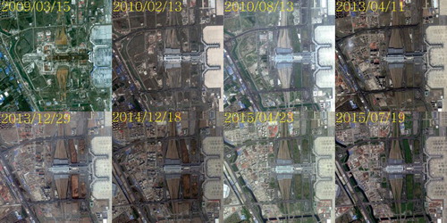
Figure 8 illustrates the changes that have occurred at the Hongqiao transportation hub using a time series of optical images from various satellites. The images are taken from Google Earth to demonstrate the change that has occurred at this location between 2009 and 2015. It is clearly visible in the first image of 2009/03/15 that the construction of the train station has just begun. The rail road tracks have not been constructed and the surrounding areas are mostly covered with green vegetation. Progressing through the time series shows a continuous development of the area along the rail road and to the west of the main building (centre of the image frame). This cluster of developing blocks is identifiable from our SAR coherence analysis as well, see Figure 7.

Figure 8. Time series from optical imagery (Google Earth).

5. Conclusion

In conclusion, we have demonstrated that the aggregation of coherence estimation to average coherence values per street-block makes sense, because change/development as well as land cover seem to be related to the entities/cadastral units. Aggregation to artificial objects that cannot be found in the real world will not yield the same results.

We have shown that the coherence of a street-block can be observed over time and that it follows the development pattern on a block-by-block basis. Even though the road network that has been employed here, from OSM, does not reflect the official data or the cadastral map of Shanghai, it is still a reasonable approximation as mentioned in Section 2, and Zheng and Zheng (2014), who have identified Shanghai’s OSM dataset as ‘most complete’.

The use of this type of voluntarily shared geographic information is very valuable in the production of the presented results. People have contributed GPS tracks to deliver the units of measurement, the real-world resemblance of urban objects. These VGI data in conjunction with remotely sensed imagery are an example for digitally representing and analysing the surface of the Earth.

Using these street-blocks as the unit of measurement (each street-block gets an average coherence value for each observation) allows the calculation of the standard deviation. This indicates the variability over time. Clustering these variability measurements reveals groups/sets of street-blocks with similar behaviour as the final result in Figure 7 demonstrates.

We argue that the processing and examination of CCD on a street-block/parcel level is vital for urban planners/designers, the real estate and property markets, and developers and investors who must understand change at a level that is relevant and recognizable in a real-world context. A coherence image alone shows a rather noisy picture, users must identify buildings and street-blocks by other means.

Disclosure statement

No potential conflict of interest was reported by the authors.

ORCiD

Timo Balz http://orcid.org/0000-0002-1624-4697

Additional information

Funding

This work was supported in part by the National Natural Science Foundation of China [grant numbers 61331016 and 41174120].

References

- Anselin, L. 2005. Exploring Spatial Data with GeoDa: A Workbook. Urbana, IL: Center for Spatially Integrated Social Science (CSISS). http://www.csiss.org/.
- Anselin, L., I. Syabri, and Y. Kho. 2006. “GeoDa: An Introduction to Spatial Data Analysis.” Geographical Analysis 38 (1): 5–22. doi:10.1111/j.0016-7363.2005.00671.x.
- Bamler, R., and P. Hartl. 1998. “Synthetic Aperture Radar Interferometry.” Inverse Problems 14 (4): R1–R54. doi: 10.1088/0266-5611/14/4/001
- Brown, M., S. Sharples, J. Harding, C. J. Parker, N. Bearman, M. Maguire, D. Forrest, M. Haklay, and M. Jackson. 2013. “Usability of Geographic Information: Current Challenges and Future Directions.” Applied Ergonomics 44 (6): 855–865. doi: 10.1016/j.apergo.2012.10.013
- Elwood, S. 2008. “Volunteered Geographic Information: Future Research Directions Motivated by Critical, Participatory, and Feminist GIS.” GeoJournal 72 (3&4): 173–183. doi: 10.1007/s10708-008-9186-0
- Elwood, S., M. F. Goodchild, and D. Z. Sui. 2012. “Researching Volunteered Geographic Information: Spatial Data, Geographic Research, and New Social Practice.” Annals of the Association of American Geographers 102 (3): 571–590. doi: 10.1080/00045608.2011.595657
- Esch, T., M. Marconcini, A. Felbier, A. Roth, W. Heldens, M. Huber, M. Schwinger, H. Taubenbock, A. Muller, and S. Dech. 2013. “Urban Footprint Processor-fully Automated Processing Chain Generating Settlement Masks from Global Data of the TanDEM-X Mission.” IEEE Geoscience and Remote Sensing Letters 10 (6): 1617–1621. doi:10.1109/LGRS.2013.2272953.
- Esch, T., H. Taubenböck, A. Roth, W. Heldens, A. Felbier, M. Thiel, M. Schmidt, A. Müller, and S. Dech. 2012. “TanDEM-X Mission—New Perspectives for the Inventory and Monitoring of Global Settlement Patterns.” Journal of Applied Remote Sensing 6 (1): 61701–61702. doi:10.1117/1.JRS.6.061702.
- Gerig, G., O. Kubler, R. Kikinis, and F. A. Jolesz. 1992. “Nonlinear Anisotrophic Filtering of MRI Data.” IEEE Transactions on Medical Imaging 11 (2): 221–232. doi: 10.1109/42.141646
- Goodchild, M. F. 2007. “Citizens as Sensors: The World of Volunteered Geography.” GeoJournal 69 (4): 211–221. doi: 10.1007/s10708-007-9111-y
- Hijmans, R. 2009. “Global Administrative Areas.” Accessed December 22, 2015. http://gadm.org/.
- Hvistendahl, M. 2013. “Foreigners Run Afoul of China’s Tightening Secrecy Rules.” Science 339 (6118): 384–385. doi:10.1126/science.339.6118.384.
- OECD. 2015. OECD Urban Policy Reviews: China 2015. Paris: OECD.
- OpenStreetMap. 2014. “Open Street Map.” Accessed December 22, 2015. http://www.openstreetmap.org/copyright.
- Perona, P., and Malik, J. (1990). “Scale-space and Edge Detection Using Anisotropic Diffusion.” IEEE Transactions on Pattern Analysis and Machine Intelligence 12 (7): 629–639. doi:10.1109/34.56205.
- Taubenböck, H., T. Esch, A. Felbier, M. Wiesner, A. Roth, and S. Dech. 2012. “Monitoring Urbanization in Mega Cities from Space.” Remote Sensing of Environment 117: 162–176. doi:10.1016/j.rse.2011.09.015.
- Taubenböck, H., and M. Wiesner. 2015. “The Spatial Network of Megaregions – Types of Connectivity between Cities Based on Settlement Patterns Derived from EO-data.” Computers, Environment and Urban Systems 54: 165–180. doi:10.1016/j.compenvurbsys.2015.07.001.
- Tobler, W. R. 1970. “A Computer Movie Simulating Urban Growth in the Detroit Region.” Economic Geography 46: 234–240. doi:10.1126/science.11.277.620.
- Wang, T., M. Liao, and D. Perissin. 2010. “InSAR Coherence-Decomposition Analysis.” IEEE Geoscience Remote Sensing Letters 7 (1): 156–160. doi: 10.1109/LGRS.2009.2029126
- Zheng, S., and J. Zheng. 2014. “Assessing the Completeness and Positional Accuracy of OpenStreetMap in China, (41361084).” doi:10.1007/978-3-319-08180-9.
- Zhou, P., W. Huang, and J. Jang. 2014. “Validation Analysis of OpenStreetMap Data in Some Areas of China.” The International Archives of the Photogrammetry, Remote Sensing and Spatial Information Sciences XL-4: 383–391. doi:10.5194/isprsarchives-XL-4-383-2014.