Mapping frequent spatio-temporal wind profile patterns using multi-dimensional sequential pattern mining

ABSTRACT

Holistic understanding of wind behaviour over space, time and height is essential for harvesting wind energy application. This study presents a novel approach for mapping frequent wind profile patterns using multi-dimensional sequential pattern mining (MDSPM). This study is illustrated with a time series of 24 years of European Centre for Medium-Range Weather Forecasts European Reanalysis-Interim gridded (0.125° × 0.125°) wind data for the Netherlands every 6 h and at six height levels. The wind data were first transformed into two spatio-temporal sequence databases (for speed and direction, respectively). Then, the Linear time Closed Itemset Miner Sequence algorithm was used to extract the multi-dimensional sequential patterns, which were then visualized using a 3D wind rose, a circular histogram and a geographical map. These patterns were further analysed to determine their wind shear coefficients and turbulence intensities as well as their spatial overlap with current areas with wind turbines. Our analysis identified four frequent wind profile patterns. One of them highly suitable to harvest wind energy at a height of 128 m and 68.97% of the geographical area covered by this pattern already contains wind turbines. This study shows that the proposed approach is capable of efficiently extracting meaningful patterns from complex spatio-temporal datasets.

KEYWORDS:

• Spatio-temporal data mining
• multi-dimensional sequential pattern mining
• wind shear coefficient
• turbulence intensity
• wind energy

1. Introduction

Wind is one of the most important renewable and ‘green’ energy sources and, as such, it is widely used for generating electricity all over the world. The global growth of wind energy production will continue in the future because the use of this renewable source of energy is actively promoted by various institutions and associations (EWEA 2014). However, there are three main contentious issues associated with the development of wind energy: (1) discovering the trend of wind patterns (Tchinda et al. 2000; Tchinda and Kaptouom 2003), (2) minimizing negative environmental impact by developing appropriate wind farm site selection criteria (Hwang et al. 2011; Kaldellis et al. 2013; Gimpel et al. 2015; Latinopoulos and Kechagia 2015) and (3) identifying the environment impact of wind farms (Dai et al. 2015).

Most wind energy studies concentrate on investigating suitable farm sites since finding viable land is a key constraint (Grassi, Chokani, and Abhari 2012; Sánchez-Lozano, García-Cascales, and Lamata 2016). Other studies have focused on the negative effects of wind farms (Sovacool 2009; Zhou et al. 2012; Chias and Abad 2013; Landscape Institute 2013).

However, erratic production of wind energy still remains as one of the main issues due to the variability of wind speed and direction over time (Fadare 2010; Jung and Tam 2013;Ozelkan, Chen, and Ustundag 2016). Hence, accurate estimation of wind energy potential is also directly involved with the wind patterns which explain the variability of wind behaviour. For a given location, the temporal trend of wind speed and direction across multiple heights is captured through a typical wind profile pattern. The identification of such profiles is essential for several applications (Tamura et al. 2001). For instance, these profiles are used to understand typical wind conditions at a single hub-height or within the swept rotor area of a wind turbines (Wagner et al. 2009). Several studies (often related to wind energy production) have been conducted to describe the characteristics of frequent wind distributions patterns (Damousis et al. 2004; Apt 2007; Carta, Ramírez, and Velázquez 2009; Krishna 2009). However, an efficient procedure to understand wind properties in these three dimensions (spatial, temporal and height) is still lacking due to the complexity of characterizing changeable and intermittent wind flows (Wagner et al. 2010).

Earlier studies of wind profile patterns included shape-dependent characteristics (Clobes, Willecke, and Peil 2011), and parameterization approaches that modelled wind profiles using logarithmic law functions (Pérez et al. 2005) or the local maxima (Kettle 2014). However, these studies are location specific (i.e. based on a single tall-tower meteorological weather station) and, hence, the revealed information is not representative for large areas (Ayotte, Davy, and Coppin 2001; Sempreviva, Barthelmie, and Pryor 2008; Newman and Klein 2014). A possible way to discover wind profile patterns with large coverage of spatial representation is using spatio-temporal pattern mining to capture frequent wind patterns continuously over time.

Spatio-temporal pattern mining offers computationally efficient approaches to identify frequent spatial and temporal patterns from large databases (Aggarwal 2014; Akbari, Samadzadegan, and Weibel 2015). In particular, sequential pattern mining (SPM) can be used to detect frequent sequential patterns. SPM has been used for a wide range of applications such as in wireless sensor, tourism science and movement patterns (Azhar et al. 2013; Bermingham and Lee 2014; Shaw and Gopalan 2014), but the usage of this technique for wind studies is still limited. Yusof et al. (2016) used SPM for detecting spatio-temporal frequent patterns in time series of wind measurements collected at a given height. However, this approach cannot deal with three-dimensional (wind) time series. To do so, multi-dimensional sequential pattern mining (MDSPM) is required. Several MDSPM techniques have been utilized in previous studies. For instance, Yu and Chen (2005) mined sequential patterns from a multi-dimensional dataset. These datasets were transformed into a simplified sequence format that belongs to a single hierarchized dimension. However, this work only extracted frequent sequential patterns that take only a single dimension into consideration. Pinto et al. (2001) used the dimensional partitioning method and the extracted sequential patterns by this technique do not retain all the dimensions. However, generating a complete set of multi-dimensional sequential patterns is important which provide specialized details about the underlying structure patterns in the data rather than too general patterns (Cai et al. 2014). Peng and Liao (2009) extracted multi-dimensional sequential patterns from the combination of multiple-dimensional information. This combination may generate large sequences. However, mining sequential patterns is inefficient with long sequences and often may not find exact matching of long patterns in the database (Kum et al. 2003). Due to these shortcomings, an improved MDSPM technique is required to mine patterns without loosing important information carried by the dimensions. This is particularly important for domains, such as wind energy studies, where reasoning about the structure of the multiple dimensions of the data and the relations between them are inherently required.

In this study, we present a novel technique for identifying wind profile patterns utilizing an MDSPM that considers changes in wind speed and direction across the three dimensions of the data (space, time and height). To the best of our knowledge, this is the first study that mines multi-dimensional geographical data by explicitly and holistically considering their spatial and temporal dimensions. This allows us to discover more complex wind behaviour associated to these dimensions. Moreover, the selected application demonstrates the value of multi-dimensional data mining in the field of renewable energies. More precisely, the proposed technique able to support the early stages of planning to develop new wind farms. Additionally, the mined frequent wind profile patterns from the proposed MDSPM are visualized using a 3D wind rose and circular histogram. After evaluating energy-relevant wind characteristics, the best patterns are used to create a map that highlights optimal areas and heights to harvest wind energy. Finally, we compare these maps with the existing location of wind turbines in the study area to verify the mined patterns.

2. Materials and methods

2.1. Study area and wind data

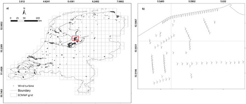
The study area comprises the whole of the Netherlands, a western European country that lies between latitudes 50° and 53°N, and longitudes 3° and 8°E (Figure 1). In 2014, the installed wind capacity in the Netherlands reached nearly 2700 MW. This means that about 5% of the energy used in the country comes from wind turbines (IEA 2014). However, wind energy is expected to steadily increase in the coming years because the national energy policy target aims at reaching 6000 MW of wind capacity on land by 2020 to meet European Union agreements (14% of renewable energy) (IEA 2014). This means that additional research is needed to understand wind patterns in the Netherlands. For this study, wind data comprising wind speed and direction were used as they are the main parameters for determining efficient wind energy production. The wind dataset used in this study was freely obtained from the European Reanalysis (ERA)-Interim reanalysis database (http://apps.ecmwf.int/datasets/data/interim-full-daily/?levtype=ml) that covers the period from 1990 to 2013. This gridded database is produced by the European Centre for Medium-Range Weather Forecasts (ECMWF) since 1 January 1989 and it contains global weather data at multiple altitudes and at various time stamps (Dee et al. 2011). The ECMWF wind dataset has been widely used as an alternative to surface-based observations such as in wind resources estimation studies (Kiss, Varga, and Janosi 2009; Cannon et al. 2015), and previous works (Landberg et al. 2003; Brower et al. 2013) have confirmed that the wind values are highly correlated with high-quality wind measurement from tall towers. In particular, we obtained the u (eastward) and v (northward) orthogonal wind components at six different pressure levels (1012, 1009, 1004, 998, 989 and 980 hPa; selected according to the range of wind turbine heights), at the four available daily instantaneous values (00:00, 06:00, 12:00 and 18:00 Universal Time Coordinated), and at the finest possible spatial resolution (0.125°). Additionally, we obtained data on the current wind turbines installed in the Netherlands from http://www.windstats.nl/. This website lists all wind turbines and categorized them according to their power rate capacities; small ( < 100 kW), medium (100 kW–1 MW) and large (1–10 MW) (Tong 2010). Each power category has a typical height of wind turbine that ranges from 34 to 198 m.

Figure 1. (a) The boundary of The Netherlands overlaid with ECMWF ERA-Interim gridded dataset and the existing location of wind turbines and (b) the close-up view of the locations of wind turbines in the selected grid cells (red box in Figure 1(a)).

2.2. Methods

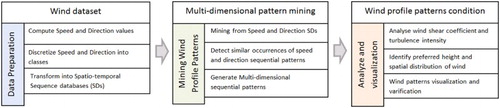
Figure 2 shows the three main steps of the proposed MDSPM approach used in this study. First, the wind dataset is transformed into spatio-temporal sequence databases. Then, these databases are mined to extract frequent wind profile patterns. Finally, the mined patterns are evaluated to identify optimal heights and locations for harvesting wind energy. The following sub-sections present the details of each of these steps.

Figure 2. Overall analytical workflow for extracting multi-dimensional wind profile patterns.

2.2.1. Data preparation

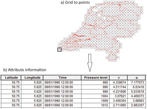
The ERA-interim dataset was clipped to extract the grid cells over the Netherlands (Figure 3(a)). The information associated to each of the grid cells (i.e. u, v, time, pressure level, latitude and longitude) were put into a tabular form (Figure 3(b)).

Figure 3. (a) Gridded ERA-Interim for the whole study area and point features representing the centre of grid cells and (b) the dimensional information which comprise latitude, longitude, time, pressure levels, u and v for a single point (point in the grey box in (a)).

The u and v orthogonal vectors were converted into wind speed (Equation (1)) and direction (Equation (2)) as these variables are more readily interpretable than the original vectors. Then, the wind speed and direction were discretized into 10 and 12 classes, respectively (Table 1). These (numbers of) classes are deemed appropriate to characterize wind distribution as confirmed by previous studies that use the exact same wind direction classes (Rijkoort 1983; Verkaik, Smits, and Ettema 2003). However, for wind speed classes were discretized according to the distribution ranges found in the wind dataset. The discretization makes the variation values of wind speed and direction more tractable by characterizing them into discrete values and allowing more patterns to be extracted which cover all the wind distributions. The pressure levels were converted into pressure altitudes in metres (Equation (3); (Brince and Hall 2009)) as this height unit is also more readily interpretable than the original unit.(1) (2) (3) where P_sta is the given pressure level in millibars.

Table 1. Wind speed and direction classes.

Speed class	Wind speed range (m/s)	Direction class	Wind direction range (°)
1	1–4	0/360°	345–14°
2	5–8	30°	15–44°
3	9–12	60°	45–74°
4	13–16	90°	75–104°
5	17–20	120°	105–134°
6	21–24	150°	135–164°
7	25–28	180°	165–194°
8	29–32	210°	195–224°
9	33–36	240°	225–254°
10	37–40	270°	255–284°
		300°	285–314°
		330°	315–344°

The new assigned values of speed and direction along with other dimensional information were stored into sequence databases. An sequence database (SD) contains a set of multi-dimensional sequences (M-DSeqs), where each of the M-DSeq is an ordered non-empty list of itemsets. These sequences were stored as rows in an SD and, therefore, they get assigned with a unique ID (ID) for each sequence which is defined as:

We have produced two SDs which consist of M-DSeqs of wind speed and direction, respectively. The multi-dimensional information for each SD consists of (a) latitude and longitude (lat, long) that contain the locations of the wind event that takes place, (b) the time holds the occurrences’ time (date and hour) and (c) the heights indicate the wind speed/direction values arranged according to their corresponding height levels. For instance, the first M-DSeq for speed and direction SDs are as follows:

Once the generated SDs are ready, they were used as the input in the mining process for extracting wind profile patterns.

2.2.2. Mining wind profile patterns

The wind speed and direction SDs were mined using a multi-dimensional frequent SPM technique that consists of three main steps: (1) mine frequent sequential patterns from wind speed and direction SDs independently, (2) Find patterns that occur at the same place and time and (3) mine and visualize frequent wind profiles patterns. Figure 4 illustrates the inputs, outputs and parameters required at each step.

Figure 4. The MDSPM workflow.

Step 1 Mining sequential patterns

Frequent sequential patterns were mined from the speed and direction of SDs (SSD and DSD, respectively) using the Linear time Closed Itemset Miner Sequence (LCMSeq) algorithm.

This algorithm was chosen because it provides fast frequency counting and requires less memory usage than other sequence pattern algorithms when mining large SDs. This is achieved by combining three computational techniques, namely prefix tree, array list and bitmaps (Uno, Kiyomi, and Arimura 2005). As a result, the time required to generate the sequential patterns is linearly proportional to the size of the input database. This reduces the computation time compared to other sequential mining algorithms (Nakahara, Uno, and Yada 2010). Moreover, the LCMSeq algorithm performs a closed search of frequent patterns. This means that it only returns patterns that are not included in longer patterns (i.e. it avoids generating redundant patterns). From a practical point of view, running this data mining algorithm only requires the definition of three parameters: the minimum support threshold (min_sup), the sequence length (SeqL) and the sequence gap (SeqG). The min_sup determines if a pattern is frequent enough to be mined. After several trials, we set the min_sup to 40% of the total data. This value generated frequent patterns that are compact and carry representative set of wind patterns that can be found in the wind dataset. The SeqL parameter defines the length of the pattern to be mined. Here, the SeqL value was fixed to six because that is the number of heights in the wind data and we are interested in mining full wind profiles. Finally, the SeqG parameter allows the user to specify the length of possible gaps or discontinuities in the patterns. This parameter was made equal to zero because, again, we are interested in mining full wind profile patterns.

Step 2 Detect similar spatio-temporal occurrences

The mined frequent sequential patterns from SSD and DSD were ‘intersected’ to identify patterns that occur at the same location together with the time of their occurrences. All the wind speed and direction patterns that intersected were combined into a set of candidate multi-dimensional sequential patterns. Figure 4 shows two examples of candidate patterns (N₁ and N₂).

Step 3 Generate multi-dimensional sequential pattern

The frequencies of all the candidate multi-dimensional sequential patterns were calculated and compared against a new min_sup threshold to identify frequent wind profiles. This new threshold was set to 20% by dividing the current min_sup (40%) by the number of sequence databases (2 SDs) created in step 1. This selection was used as a basic rule for providing min_sup to endure with the loosing (unmatched) patterns that occurred during the sequential combination between SSeq and DSeq. Finally, the mined wind profile patterns were visualized using a 3D wind rose and a circular histogram to illustrate their speed and direction and to highlight their occurrences over time.

2.2.3. Wind patterns analysis and visualization

The mined wind profiles were analysed to assess their potential for harnessing wind energy. For this, we computed two well-known wind characteristics from hourly and monthly wind values: the wind shear coefficient (WSC) and the turbulence intensity (TI) (Rehman and Al-Abbadi 2008; Fırtın, Güler, and Akdağ 2011). The hourly and monthly evaluations were performed in order to identify the influence of diurnal and seasonal changes in wind data.

The WSC measures changes in wind speed over a short distance that occur vertically in heights. WSC is mostly dependent on the stability of the atmosphere and surface obstruction (Elkinton, Rogers, and McGowan 2006; Istchenko and Turner 2008). The WSC value describes the atmospheric stability where at strongly stable atmospheric condition it corresponds to high wind shear. Meanwhile, at strongly unstable atmospheric condition it is relatively the result of lowest wind shear (Smith et al. 2002; Newman and Klein 2014). Knowing this value is essential for evaluating the wind condition at various heights which is associated to different turbine hubs. The WSC (α) can be measured as follows (Equation (4)) (Gualtieri and Secci 2011):(4) where V₁ and V₂ are the wind speed records at heights Z₁ and Z₂, respectively. To obtain the values of WSC, we have divided into six pairs of height interval comprised of α1:195–280 m, α2:128–195 m, α3:77–128 m, α4:35–77 m, α5:10–35 m and α6:10–280 m.

The TI measures irregular wind flows in which the wind whirls rapidly because of uneven terrain surface or obstacles such as buildings (Wagner and Mathur 2013). These whirls can be different between the wind flows at different heights (Carpman 2011). A maximum TI indicates lowest wind speed when the wind flow is encountered by surface obstructions. This effect decreases with increasing height above the surface. Consequently, as TI minimizes, wind speed increases (Gipe 2004; Sørensen 2007). Measuring TI is important because larger amount of turbulence will generate a larger amount of fatigue that, in turn, increases the rate at which wind turbines break down (Wharton and Lundquist 2012). The following equation was used to assess wind turbulence (Equation (5)) (Rehman 2014; Gualtieri 2015b):(5)

where (σ_i) is the standard deviation of the wind speed within time step i and V_i is the mean wind speed in time step i .

Once the WSC (α) and TI values of the wind profile patterns are known, these values were classified according to the wind stability and speed condition. For this, we used the criteria developed by Wharton and Lundquist (2012) shown in Table 2. From these classifications, we are able to evaluate the vertical wind condition for each wind pattern and identify their preferred height wind speed that is suitable to harvest wind energy. Afterwards, the wind patterns were mapped into the geographic space to indicate their spatial distribution, while the total numbers of pattern occurrences in each cell (Figure 3(a)) were computed in percentage to represent the wind patterns over time. For the verification, these maps were overlapped with the existing locations of wind turbines and presented in a bar chart to illustrate the percentage of overlapping areas.

Table 2. Threshold values of WSC (α) and TI for major wind condition classification.

Wind shear (α)	Stability class	Turbulence intensity (TI)	Wind speed condition
Highest : α > 0.3	Strongly stable	Lowest : TI < 4%	Strongest
High : 0.2 < α < 0.3	Stable	Low : 4% < TI < 6%	Strong
Moderate : 0.1 < α < 0.2	Near-neutral	Moderate : 6% < TI < 9%	Generally Calm
Low : 0.0 < α < 0.1	Convective	High : 9% < TI < 17%	Low
Lowest : α < 0.0	Strongly convective	Highest : TI > 17%	Lowest

3. Results and discussion

3.1. Data analysis

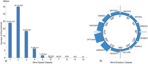
The extracted ECMWF gridded values that were saved into tabular form consists of 85,836,672 records (on average of 3,576,528 records per year). Figure 5(a) and (b) illustrates the frequency distribution of wind speeds and direction after discretizing them into 10 and 12 classes, respectively. From this figure, we observed that wind speed in class 2 (5–8 m/s) is the dominant speed followed by class 1 (1–4 m/s) and 3 (9–12 m/s) for the whole time period. However, the wind rose plot indicates that the prevailing wind direction mostly comes from the westerly wind, while the easterly wind direction shows a somewhat similar number of occurrences.

Figure 5. Total occurrences for (a) wind speed classes and (b) wind direction classes.

The discretized wind speed and direction data were stored in separate sequence databases following the format described in Section 2.2.1, which is { < ID > , < lat, long > , < time > , < heights of wind speed/direction > }. Hence, each SD contains a total of 14,306,112 sequences (i.e. the total records divided by six height levels).

3.2. Mining wind profile patterns

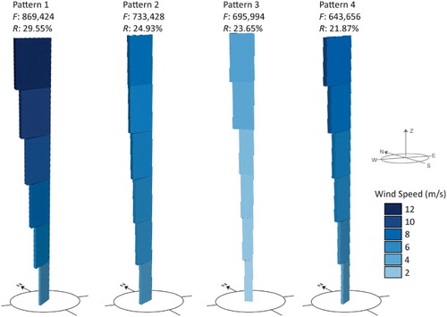
The application of LCMSeq to the speed and direction SDs resulted in five unique sequential patterns for each of the sequence databases (SSeq and DSeq, respectively). These unique patterns represent a total of 48% (SSeq) and 41% (DSeq) of occurrences. The spatio-temporal intersection of the SSeq and DSeq patterns identified a total of 25 candidates of multi-dimensional sequential patterns. Only four of these patterns have a frequency larger than 20%. Hence, these selected patterns are used to represent the wind profile patterns. Figure 6 shows the corresponding wind profiles and their corresponding absolute and relative frequencies.

Figure 6. The extracted wind profile patterns and their number of occurrences (absolute (F) and relative (R) frequencies) obtained from the MDSPM process.

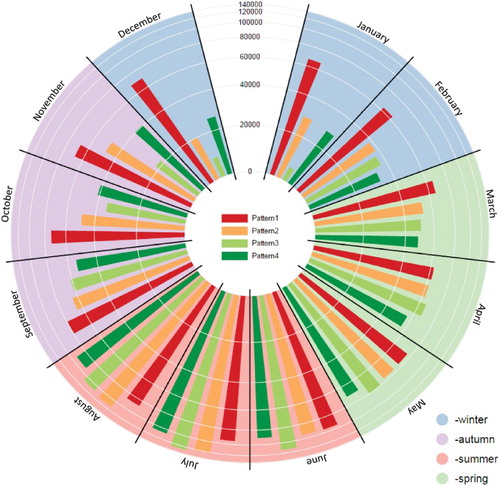
Figure 7 shows the absolute frequency of these four wind profile patterns in each month of the year and highlights the seasonality of the patterns. Pattern 1 dominates the number of occurrences in January to March (winter–spring) and from September to December (autumn–winter). During summer, there are increased numbers of occurrences for all wind profile patterns compared to other seasons. However, pattern 3 depicts the dominant pattern in this season. Overall, pattern 1 shows more consistency based on the occurrences over time compared to other patterns.

Figure 7. Circular histogram of the wind profile patterns for each month of the year and season.

3.3. Analysis of wind profile patterns and visualization

The mined wind profile patterns were analysed in hourly and monthly wind values. Figures 8 and 9 show the results of the WSC and TI of the mined wind patterns. The results for pattern 1 at the hourly (Figure 8(a)) and monthly (Figure 8(b)) temporal resolutions show very slight differences of WSCs at various height intervals. The WSC shows larger values in the early morning (0 and 6 h) and evening (18 h). However, the WSCs in the afternoon (12 h) are moderate. During the warm seasons (June, July and August) pattern 1 has moderate wind shear while it depicts high wind shear for the rest of the months in all height intervals. The decreased wind shear is due to unstable atmosphere stability that is affected by heating and cooling cycles of air above the ground (van den Berg 2008). These results are confirmed by the meteorological mass tower at Cabauw (Netherlands) studied by Gualtieri (2015a). Pattern 2 depicts nearly constant WSC values over time. In general, higher values of WSC were noticed at lower heights as shown in Figure 8(a) and (b). For pattern 3, the fluctuation of WSC values can be observed in hourly temporal resolution. However, in the monthly resolution the WSC values appear to be slightly stable. Higher values of WSC were observed at upper heights intervals (Figure 8(a) and (b)). The overall trend for pattern 4 is similar to pattern 1 for hourly resolution of WSCs (Figure 8(a)). However, the monthly resolution shows slightly constant WSC values throughout the year and fall in the moderate wind shear category.

Figure 8. (a) Wind shear coefficient at four instantaneous hours (0, 6, 12 and 18 h) for each wind profile pattern at six different height intervals and (b) Wind shear coefficient for each wind profile pattern at six different height intervals for every month of the year.

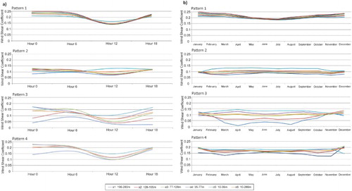
Figure 9. (a) Turbulence intensity at four instantaneous hours (0, 6, 12 and 18 h) for each wind profile pattern at six different heights and (b) Turbulence intensity for each wind profile pattern at six different heights for every month of the year.

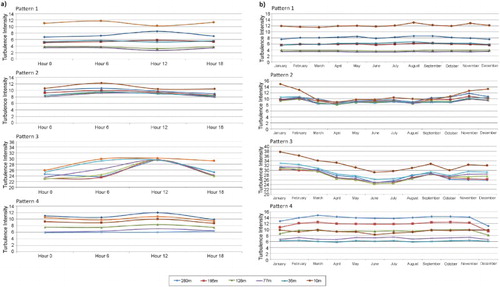
The observed TI values remained stable in both hourly (Figure 9(a)) and monthly (Figure 9(b)) temporal resolutions in pattern 1. As shown, the TI is smoother at upper heights (TI₇₇ and TI₁₂₈) and consists of lower values. Pattern 2 shows higher TI values for hourly resolution at all heights. If compared to the corresponding WSC one (Figure 8(a)), the following features affect the hourly TI trend: (i) a quite constant behaviour in daytime and night-time and (ii) slight differences among TI at various heights vs. WSCs at various height intervals. The TI by monthly resolution (Figure 8(b)) also depicts high values and its shape does not appreciably vary with heights. Pattern 3 depicts the highest TI values at all height levels throughout the time resolutions (Figure 9(a) and 9(b)). High TI indicates a good mixture of atmospheric stability conditions at each height. For pattern 4, a similar trend can be observed in both hourly and monthly resolution at all consecutive heights. Lower TI values were observed at lower heights (increase of TI as height increases which spans from 6% (TI₃₅) to 15% (TI₂₈₀)). This trend is formed as turbulence eddies (Burton et al. 2001).

Table 3 summarizes the main findings of the evaluation of the mined wind profile patterns in terms of WSC and TI. This table lists the most suitable conditions for every wind pattern.

Table 3. Selected mean of WSC and TI for wind patterns.

Pattern	Category: WSC and TI	Height
Hourly
Pattern 1	High (0.24) and Lowest (3.67)	128 m
Pattern 2	Moderate (0.11) and Moderate (8.56)	77 m
Pattern 3	Moderate (0.12) and Highest (25.15)	128 m
Pattern 4	High (0.20) and Moderate (6.05)	35 m
Monthly
Pattern 1	High (0.23) and Lowest (3.84)	128 m
Pattern 2	Moderate (0.10) and Moderate (8.63)	77 m
Pattern 3	Moderate (0.11) and Highest (28.09)	128 m
Pattern 4	Moderate (0.18) and Moderate (6.13)	35 m

From Table 3 summarization, we can identify that pattern 1 shows the best results of WSC and TI compared with the rest of the wind patterns. The wind behaviour for this pattern is considered as a strong wind and has a stable atmospheric stability condition at the selected 128 m height. Additionally, pattern 1 also exhibited high frequency of occurrences over time which may indicate a regular wind behaviour that occurred in the study area. This finding indicates that wind speed at the selected height is the preferred height for wind resources potential. For pattern 2, the selected wind condition was identified at 77 m height, which consists of calm wind flow and near to neutral stability condition. However, for pattern 3 the selected height at 128 m shows that the wind behaviour is in a near to neutral stability condition with low wind velocity. Additionally, the selected height at 35 m that corresponded to pattern 4 consists of stable and calm wind flow condition.

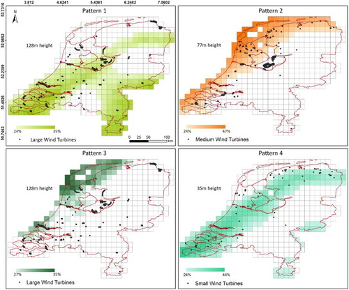
Moreover, the analysed wind patterns, based on the assessment of WSC and TI (Table 3), were mapped into their geographical space and overlapped with the existing locations of wind turbines according to the turbine categories. Figure 10 illustrates the distribution of wind patterns that correspond to their height. The figure also depicts the percentage of wind pattern occurrences in each cell over time. The highest percentage of occurrences for pattern 1 is concentrated in the south and southwest of the Netherlands. The wind occurrences for pattern 2 are mostly distributed adjacent to the coastal area of the Netherlands which also can be observed in pattern 3; however, both of these patterns are located at different heights. For pattern 4, there are several minor parts of the wind occurrences located in the eastern and southern area, whereas the rest of the occurrences are distributed in the north and southwest of the Netherlands.

Figure 10. The wind patterns distribution based on their height and the percentage of occurrences over time in each grid cell overlaid on top of wind turbine locations.

Figure 11 illustrates the percentage of overlapping areas between the wind patterns and the locations of wind turbines for verifying the geographical distribution of the mined patterns. The generated maps for pattern 1 show the highest percentage of overlapping with 68.97%, followed by pattern 4 (59.18%) and 2 (43.87%). However, pattern 3 resulted in the lowest percentage (22.25%). The small overlapping areas can be affected by other factors such as the geographical features, social condition and land use activities, which influence the positioning of the wind turbines. From these verifications, this study indicates that pattern 1 distribution was prone to most of the wind turbine locations in the study area.

Figure 11. The percentage of overlap between current wind turbine locations and the geographic distribution of the mined wind profile patterns.

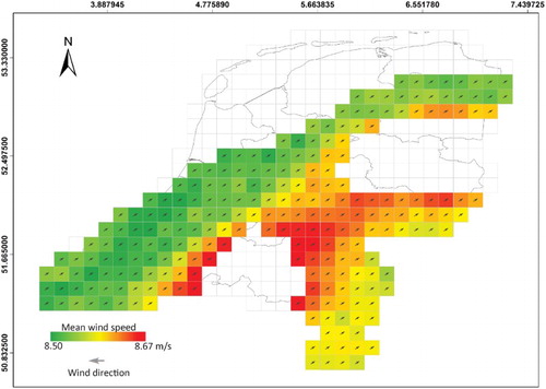
The geographical distribution of wind speed and direction associated to pattern 1 is illustrated in Figure 12. This preferred pattern contains mean wind speed that range from 8.50 to 8.67 m/s and the highest (red colour) wind speeds are mostly found in the middle part of the Netherlands. The predominant wind direction indicates that wind mainly blows from the southwest direction.

Figure 12. The geographical distribution of mean wind speed and wind direction for pattern 1 at a 128 m height from the surface.

4. Conclusion

The exploration of wind profile patterns in the early stage of wind farm planning is one of the key elements for gaining a better understanding of the wind condition. Besides, the generated wind pattern yields users useful qualitative information about wind behaviour which in turn can provide knowledge to experts. This study demonstrates a novel approach to mine and map frequent wind profile patterns. This approach, based on the use of sequential data mining, was illustrated with a time series of 24-year of ECMWF ERA-Interim wind data for the Netherlands. Results show that there are four main wind profile patterns in the study area. The WSC and TI of these patterns were analysed to evaluate their suitability to harvest wind energy. From this analysis we concluded that only wind profile pattern 1 at 128 m of height is sufficiently strong and stable for generating sufficient wind energy. Fortunately, this pattern is the most dominant one (i.e. has the highest occurrences and it is consistently found over time). Moreover, the spatial coverage of pattern 1 largely overlaps (∼69%) with the actual location of wind turbines.

This work represents a first attempt at implementing MDSPM for assessing wind profile patterns over large areas. The mined wind profiles are particularly useful to quantify wind resource potential at various heights, and this information is essential for early stage planning of wind farms. The proposed MDSPM approach is generic: it can be applied to other locations and even to other spatio-temporal problems thanks to its two main hallmarks: (1) it can mine patterns from n-dimensional datasets (i.e. it can be can be applied to spatio-temporal data with more than 3 dimensions) and (2) it allows a quick and deep understanding of the mined patterns by combining data mining and a suite of visualizations, namely the 3D wind rose, the circular histogram and geographical maps.

Regarding the applicability to other locations, the proposed approach can potentially be applied globally because it only requires gridded wind data at various heights. Yet, areas with complex relief might require finer spatial resolutions than the ones currently provided by the ECMWF and the application of MDSPM to large areas might be computationally challenging.

Acknowledgements

The authors would like to acknowledge the European Centre for Medium-Range Weather Forecasts (ECMWF) for providing the wind dataset.

Disclosure statement

No potential conflict of interest was reported by the authors.

Additional information

Funding

This work was supported by the Malaysian Ministry of Education (SLAI) and Universiti Teknologi Malaysia (UTM).

References

- Aggarwal, Charu C. 2014. “An Introduction to Frequent Pattern Mining.” In Frequent Pattern Mining, edited by Charu C. Aggarwal and Jiawei Han, 1–17. Basel: Springer International.
- Akbari, M., F. Samadzadegan, and R. Weibel. 2015. “A Generic Regional Spatio-Temporal co-Occurrence Pattern Mining Model: A Case Study for air Pollution.” Journal of Geographical Systems 17 (3): 249–274. doi:10.1007/s10109-015-0216-4.
- Apt, Jay. 2007. “The Spectrum of Power from Wind Turbines.” Journal of Power Sources 169 (2): 369–374. doi:10.1016/j.jpowsour.2007.02.077.
- Ayotte, KeithW, Robert J. Davy, and Peter A. Coppin. 2001. “A Simple Temporal and Spatial Analysis of Flow in Complex Terrain in the Context of Wind Energy Modelling.” Boundary-Layer Meteorology 98 (2): 275–295. doi:10.1023/A:1026583021740.
- Azhar, Mahmood, Shi Ke, Khatoon Shaheen, and Xiao Mi. 2013. “Data Mining Techniques for Wireless Sensor Networks: A Survey.” International Journal of Distributed Sensor Networks 9 (7): 1–24.
- van den Berg, G. P. 2008. “Wind Turbine Power and Sound in Relation to Atmospheric Stability.” Wind Energy 11 (2): 151–169. doi:10.1002/we.240.
- Bermingham, Luke, and Ickjai Lee. 2014. “Spatio-temporal Sequential Pattern Mining for Tourism Sciences.” Procedia Computer Science 29: 379–389. doi:10.1016/j.procs.2014.05.034.
- Brince, Tim, and Todd Hall. 2009. “Pressure Altitude.” Accessed January 2015. http://www.srh.noaa.gov/epz/?n=wxcalc_pressurealtitude.
- Brower, M. C. , M. S. Barton, L. Lledó, and J. Dubois. 2013. “ A Study of Wind Speed Variability Using Global Reanalysis Data.” AWS Truepower technical report.
- Burton, T., D. Scarpe, N. Jenkins, and E. Bossanyi. 2001. Wind Energy Handbook. Chichester: John Wiley.
- Cai, Guochen, Chihiro Hio, Luke Bermingham, Kyungmi Lee, and Ickjai Lee. 2014. “Sequential Pattern Mining of geo-Tagged Photos with an Arbitrary Regions-of-Interest Detection Method.” Expert Systems with Applications 41 (7): 3514–3526. doi:10.1016/j.eswa.2013.10.057.
- Cannon, D. J., D. J. Brayshaw, J. Methven, P. J. Coker, and D. Lenaghan. 2015. “Using Reanalysis Data to Quantify Extreme Wind Power Generation Statistics: A 33 Year Case Study in Great Britain.” Renewable Energy 75 (0): 767–778. doi:10.1016/j.renene.2014.10.024.
- Carpman, N. 2011. Turbulence Intensity in Complex Environments and its Influence on Small Wind Turbines. Department of Earth Sciences Geotryckeriet, Uppsala University. Uppsala: Uppsala University.
- Carta, J. A., P. Ramírez, and S. Velázquez. 2009. “A Review of Wind Speed Probability Distributions Used in Wind Energy Analysis: Case Studies in the Canary Islands.” Renewable and Sustainable Energy Reviews 13 (5): 933–955. doi:10.1016/j.rser.2008.05.005.
- Chias, Pilar, and Tomás Abad. 2013. “Wind Farms: GIS-Based Visual Impact Assessment and Visualization Tools.” Cartography and Geographic Information Science 40 (3): 229–237. doi:10.1080/15230406.2013.809231.
- Clobes, Mathias, Andreas Willecke, and Udo Peil. 2011. “Shape-dependent Characteristics of Full-Scale Wind Profiles.” Journal of Wind Engineering and Industrial Aerodynamics 99 (9): 919–930. doi:10.1016/j.jweia.2011.05.005.
- Dai, Kaoshan, Anthony Bergot, Chao Liang, Wei-Ning Xiang, and Zhenhua Huang. 2015. “Environmental Issues Associated with Wind Energy – A Review.” Renewable Energy 75: 911–921. doi:10.1016/j.renene.2014.10.074.
- Damousis, I. G., M. C. Alexiadis, J. B. Theocharis, and P. S. Dokopoulos. 2004. “A Fuzzy Model for Wind Speed Prediction and Power Generation in Wind Parks using Spatial Correlation.” IEEE Transactions on Energy Conversion 19 (2): 352–361. doi:10.1109/TEC.2003.821865.
- Dee, D. P., S. M. Uppala, A. J. Simmons, P. Berrisford, P. Poli, S. Kobayashi, U. Andrae, et al. 2011. “The ERA-Interim Reanalysis: Configuration and Performance of the Data Assimilation System.” Quarterly Journal of the Royal Meteorological Society 137 (656): 553–597. doi:10.1002/qj.828.
- Elkinton, M. R., A. L. Rogers, and J. G. McGowan. 2006. “An Investigation of Wind-Shear Models and Experimental Data Trends for Different Terrains.” Wind Engineering 30 (4): 341–350. doi:10.1260/030952406779295417.
- EWEA (European Wind Energy Association). 2014. Wind Power 2014 European Statistics. Brussels: The European Wind Energy Association.
- Fadare, D. A. 2010. “The Application of Artificial Neural Networks to Mapping of Wind Speed Profile for Energy Application in Nigeria.” Applied Energy 87 (3): 934–942. doi:10.1016/j.apenergy.2009.09.005.
- Fırtın, Ebubekir, Önder Güler, and Seyit Ahmet Akdağ. 2011. “Investigation of Wind Shear Coefficients and Their Effect on Electrical Energy Generation.” Applied Energy 88 (11): 4097–4105. doi:10.1016/j.apenergy.2011.05.025.
- Gimpel, Antje, Vanessa Stelzenmüller, Britta Grote, Bela H. Buck, Jens Floeter, Ismael Núñez-Riboni, Bernadette Pogoda, and Axel Temming. 2015. “A GIS Modelling Framework to Evaluate Marine Spatial Planning Scenarios: Co-Location of Offshore Wind Farms and Aquaculture in the German EEZ.” Marine Policy 55: 102–115. doi:10.1016/j.marpol.2015.01.012.
- Gipe, Paul. 2004. Wind Power: Renewable Energy for Home, Farm, and Business, 2nd Edition. 2nd ed., Measuring the Wind. White River Junction: Chelsea Green
- Grassi, Stefano, Ndaona Chokani, and Reza S. Abhari. 2012. “Large Scale Technical and Economical Assessment of Wind Energy Potential with a GIS Tool: Case Study Iowa.” Energy Policy 45: 73–85. doi:10.1016/j.enpol.2012.01.061.
- Gualtieri, Giovanni. 2015a. “The Strict Relationship between Surface Turbulence Intensity and Wind Shear Coefficient Daily Courses: A Novel Method to Extrapolate Wind Resource to the Turbine Hub Height.” International Journal of Renewable Energy Research 5 (1): 183–200.
- Gualtieri, Giovanni. 2015b. “Surface Turbulence Intensity as a Predictor of Extrapolated Wind Resource to the Turbine hub Height.” Renewable Energy 78 (0): 68–81. doi:10.1016/j.renene.2015.01.011.
- Gualtieri, Giovanni, and Sauro Secci. 2011. “Comparing Methods to Calculate Atmospheric Stability-Dependent Wind Speed Profiles: A Case Study on Coastal Location.” Renewable Energy 36 (8): 2189–2204. doi:10.1016/j.renene.2011.01.023.
- Hwang, G. H., L. S. Wei, K. B. Ching, and N. S. Lin. 2011. “Wind Farm Allocation in Malaysia Based on Multi-Criteria Decision Making Method.” Paper presented at the National Postgraduate Conference (NPC), Universiti Teknologi PETRONAS, Perak, Malaysia, September 19–20.
- IEA (International Energy Agency). 2014. IEA Wind Annual Report 2014. The Netherlands. The International Energy Agency.
- Istchenko, Rob, and Barry Turner. 2008. “Extrapolation of Wind Profiles using Indirect Measures of Stability.” Wind Engineering 32 (5): 433–438. doi:10.1260/030952408786411967.
- Jung, Jaesung, and Kwa-Sur Tam. 2013. “A Frequency Domain Approach to Characterize and Analyze Wind Speed Patterns.” Applied Energy 103: 435–443. doi:10.1016/j.apenergy.2012.10.006.
- Kaldellis, J. K., M. Kapsali, El Kaldelli, and Ev Katsanou. 2013. “Comparing Recent Views of Public Attitude on Wind Energy, Photovoltaic and Small Hydro Applications.” Renewable Energy 52: 197–208. doi:10.1016/j.renene.2012.10.045.
- Kettle, Anthony J. 2014. “Unexpected Vertical Wind Speed Profiles in the Boundary Layer Over the Southern North Sea.” Journal of Wind Engineering and Industrial Aerodynamics 134: 149–162. doi:10.1016/j.jweia.2014.07.012.
- Kiss, P., L. Varga, and I. M. Janosi. 2009. “Comparison of Wind Power Estimates from the ECMWF Reanalyses with Direct Turbine Measurements.” Journal of Renewable and Sustainable Energy 1 (3): 033105, 1–11. doi:10.1063/1.3153903.
- Krishna, Kailasam Muni. 2009. “On the Benefits of using a High-Resolution Mesoscale Model to Improve Wind Field for the Study of Upwelling off the Indian Coasts.” International Journal of Digital Earth 2 (2): 122–133. doi:10.1080/17538940802657702.
- Kum, H.-C., J. Pei, W. Wang, and D. Duncan. 2003. “ApproxMAP: Approximate Mining of Consensus Sequential Patterns.” Paper presented at the 2003 SIAM International Conference on Data Mining (SDM ‘03), Cathedral Hill Hotel, San Francisco, CA, May 1–3.
- Landberg, L., L. Myllerup, O. Rathmann, E. L. Petersen, B. H. Jorgensen, J. Badger, and N. G. Mortensen. 2003. “Wind Resource Estimation – An Overview.” Wind Energy 6 (3): 261–271. doi:10.1002/we.94.
- Landscape Institute. 2013. Guidelines for Landscape and Visual Impact Assessment. 3rd ed. Abingdon: Routledge Taylor & Francis.
- Latinopoulos, D., and K. Kechagia. 2015. “A GIS-Based Multi-Criteria Evaluation for Wind Farm Site Selection. A Regional Scale Application in Greece.” Renewable Energy 78: 550–560. doi:10.1016/j.renene.2015.01.041.
- Nakahara, Takanobu, Takeaki Uno, and Katsutoshi Yada. 2010. “Extracting Promising Sequential Patterns from RFID Data Using the LCM Sequence.” In Knowledge-Based and Intelligent Information and Engineering Systems, edited by Rossitza Setchi, Ivan Jordanov, Robert J. Howlett and Lakhmi C. Jain, 244–253. Berlin: Springer.
- Newman, Jennifer, and Petra Klein. 2014. “The Impacts of Atmospheric Stability on the Accuracy of Wind Speed Extrapolation Methods.” Resources 3 (1): 81–105. doi: 10.3390/resources3010081
- Ozelkan, Emre, Gang Chen, and Burak Berk Ustundag. 2016. “Spatial Estimation of Wind Speed: A new Integrative Model using Inverse Distance Weighting and Power law.” International Journal of Digital Earth 9 (8): 733–747. doi:10.1080/17538947.2015.1127437.
- Peng, Wen-Chih, and Zhung-Xun Liao. 2009. “Mining Sequential Patterns Across Multiple Sequence Databases.” Data & Knowledge Engineering 68 (10): 1014–1033. doi:10.1016/j.datak.2009.04.009.
- Pérez, I. A., M. A. García, M. L. Sánchez, and B. de Torre. 2005. “Analysis and Parameterisation of Wind Profiles in the low Atmosphere.” Solar Energy 78 (6): 809–821. doi:10.1016/j.solener.2004.08.024.
- Pinto, Helen, Jiawei Han, Jian Pei, Ke Wang, Qiming Chen, and Umeshwar Dayal. 2001. “Multi-dimensional Sequential Pattern Mining.” Paper presented at the tenth international conference on Information and knowledge management, Atlanta, Georgia, November 5–10.
- Rehman, Shafiqur. 2014. “Tower Distortion and Scatter Factors of co-Located Wind Speed Sensors and Turbulence Intensity Behavior.” Renewable and Sustainable Energy Reviews 34 (0): 20–29. doi:10.1016/j.rser.2014.03.007.
- Rehman, Shafiqur, and Naif M. Al-Abbadi. 2008. “Wind Shear Coefficient, Turbulence Intensity and Wind Power Potential Assessment for Dhulom, Saudi Arabia.” Renewable Energy 33 (12): 2653–2660. doi:10.1016/j.renene.2008.02.012.
- Rijkoort, P. J. 1983. “ A compound Weibull model for the description of surface wind velocity distributions.” Royal Netherlands Meteorological Institute (KNMI).
- Sánchez-Lozano, J. M., M. S. García-Cascales, and M. T. Lamata. 2016. “GIS-based Onshore Wind Farm Site Selection using Fuzzy Multi-Criteria Decision Making Methods. Evaluating the Case of Southeastern Spain.” Applied Energy 171: 86–102. doi:10.1016/j.apenergy.2016.03.030.
- Sempreviva, A. M., R. J. Barthelmie, and S. C. Pryor. 2008. “Review of Methodologies for Offshore Wind Resource Assessment in European Seas.” Surveys in Geophysics 29 (6): 471–497. doi:10.1007/s10712-008-9050-2.
- Shaw, Arthur A., and N. P. Gopalan. 2014. “Finding Frequent Trajectories by Clustering and Sequential Pattern Mining.” Journal of Traffic and Transportation Engineering (English Edition) 1 (6): 393–403. doi:10.1016/S2095-7564(15)30289-0.
- Smith, K., G. Randall, D. Malcolm, N. Kelley, and B. Smith. 2002. “Evaluation of Wind Shear Patterns at Midwest Wind Energy Facilities.” Conference Paper Association (AWEA) WINDPOWER 2002 Conference, Portland, Oregon, June 2–5, 2002.
- Sørensen, John Dalsgaard. 2007. Reliability and Optimization of Structural Systems: Assessment, Design and Life-Cycle Performance. London: CRS Press, Taylor & Francis Group.
- Sovacool, Benjamin K. 2009. “Contextualizing Avian Mortality: A Preliminary Appraisal of Bird and Bat Fatalities from Wind, Fossil-Fuel, and Nuclear Electricity.” Energy Policy 37 (6): 2241–2248. doi:10.1016/j.enpol.2009.02.011.
- Tamura, Yukio, Kenichi Suda, Atsushi Sasaki, Yoshiharu Iwatani, Kunio Fujii, Ryukichi Ishibashi, and Kazuki Hibi. 2001. “Simultaneous Measurements of Wind Speed Profiles at two Sites using Doppler Sodars.” Journal of Wind Engineering and Industrial Aerodynamics 89 (3–4): 325–335. doi:10.1016/S0167-6105(00)00085-4.
- Tchinda, Réné, and Ernest Kaptouom. 2003. “Wind Energy in Adamaoua and North Cameroon Provinces.” Energy Conversion and Management 44 (6): 845–857. doi:10.1016/S0196-8904(02)00092-4.
- Tchinda, Réné, Joseph Kendjio, Ernest Kaptouom, and Donation Njomo. 2000. “Estimation of Mean Wind Energy available in far North Cameroon.” Energy Conversion and Management 41 (17): 1917–1929. doi:10.1016/S0196-8904(00)00017-0.
- Tong, Wei. 2010. Wind Power Generation and Wind Turbine Design, WIT Transactions on State-of-the-art in Science and Engineering. Southampton: WITPress.
- Uno, Takeaki, Masashi Kiyomi, and Hiroki Arimura. 2005. “LCM ver.3: Collaboration of Array, Bitmap and Prefix Tree for Frequent Itemset Mining.” Paper presented at the 1st international workshop on open source data mining: frequent pattern mining implementations, Chicago, IL, August 21–24.
- Verkaik, J. W., A. Smits, and J. Ettema. 2003. “Extreme Value Analysis and Spatial Interpolation Methods for the Determination of Extreme Return Levels of Wind Speed.” KNMI-HYDRA Project: Wind Climate Assessment of the Netherlands 2003. De Bilt, Royal Netherlands Meteorological Institute (KNMI) Phase Report 9: 1–202.
- Wagner, Rozenn, Ioannis Antoniou, Søren M. Pedersen, Michael S. Courtney, and Hans E. Jørgensen. 2009. “The Influence of the Wind Speed Profile on Wind Turbine Performance Measurements.” Wind Energy 12 (4): 348–362. doi:10.1002/we.297.
- Wagner, Rozenn, Michael Courtney, Torben J. Larsen, and Uwe SchmidtPaulsen. 2010. “Simulation of Shear and Turbulence Impact on Wind Turbine Performance.” In Risø-R-Report. National Laboratory for Sustainable Enegy Risø DTU.
- Wagner, Hermann-Josef, and Jyotirmay Mathur. 2013. “Wind: Origin and Local Effects.” Chapter 2 in Introduction to Wind Energy Systems. Heidelberg: Springer.
- Wharton, S., and J. K. Lundquist. 2012. “Atmospheric Stability Affects Wind Turbine Power Collection.” Environmental Research Letters 7 (1): 014005, 1–9. doi:10.1088/1748-9326/7/1/014005.
- Yu, Chung-Ching, and Yen-Liang Chen. 2005. “Mining Sequential Patterns from Multidimensional Sequence Data.” IEEE Transaction on Knowledge and Data Engineering 17 (1): 136–140. doi:10.1109/tkde.2005.13.
- Yusof, Norhakim, Raul Zurita-Milla, Menno-Jan Kraak, and Bas Retsios. 2016. “Interactive Discovery of Sequential Patterns in Time Series of Wind Data.” International Journal of Geographical Information Science 30 (8): 1486–1506. doi:10.1080/13658816.2015.1135928.
- Zhou, Liming, Yuhong Tian, Somnath Baidya Roy, Chris Thorncroft, Lance F. Bosart, and Yuanlong Hu. 2012. “Impacts of Wind Farms on Land Surface Temperature.” Nature Climate Change 2 (7): 539–543. http://www.nature.com/nclimate/journal/v2/n7/abs/nclimate1505.html#supplementary-information.