Fine-resolution forest tree height estimation across the Sierra Nevada through the integration of spaceborne LiDAR, airborne LiDAR, and optical imagery

ABSTRACT

Forests of the Sierra Nevada (SN) mountain range are valuable natural heritages for the region and the country, and tree height is an important forest structure parameter for understanding the SN forest ecosystem. There is still a need in the accurate estimation of wall-to-wall SN tree height distribution at fine spatial resolution. In this study, we presented a method to map wall-to-wall forest tree height (defined as Lorey’s height) across the SN at 70-m resolution by fusing multi-source datasets, including over 1600 in situ tree height measurements and over 1600 km² airborne light detection and ranging (LiDAR) data. Accurate tree height estimates within these airborne LiDAR boundaries were first computed based on in situ measurements, and then these airborne LiDAR-derived tree heights were used as reference data to estimate tree heights at Geoscience Laser Altimeter System (GLAS) footprints. Finally, the random forest algorithm was used to model the SN tree height from these GLAS tree heights, optical imagery, topographic data, and climate data. The results show that our fine-resolution SN tree height product has a good correspondence with field measurements. The coefficient of determination between them is 0.60, and the root-mean-squared error is 5.45 m.

KEYWORDS:

• Tree height
• Sierra Nevada
• LiDAR
• integration
• fine resolution

1. Introduction

Forests of the Sierra Nevada (SN) mountain range, covering an area of 63,100 km², are valuable natural heritages for the region and the country. As one of the most diverse temperate conifer forests on Earth, the SN serves a series of ecosystem functions for the region and even the United States (US), for example, regulating functions by maintaining essential ecological processes and life support systems, supporting functions by providing habitats for wild plants and animals in the region, provisioning functions by supplying provisions of natural resources, and cultural functions by offering life fulfilment opportunities and cognitive developments (Bales et al. 2011). In recent decades, forests of the SN have been extensively exploited and managed to deal with the increasing wildfire risk induced by fire suppression, fuel build up, and climate change (Stephens, Millar, and Collins 2010). These forest management activities have brought growing concerns that they may destroy wildlife habitats, especially the habitats of endangered species (Berigan, Gutiérrez, and Tempel 2012; Matthews et al. 2013). Tree height, an important forest structure parameter, plays a crucial role in understanding the ecosystem of a forest and therefore modelling the wildlife habitat within the forest (Martinuzzi et al. 2009; Vierling et al. 2008).

Traditionally, forest tree heights are randomly sampled by taking accurate in situ measurements (Naesset 1997; Næsset and Økland 2002). Numerous efforts from US Forest Service (USFS) have been devoted to obtaining ground measured tree height in the SN forests, for example, the Forest Inventory and Analysis (FIA) Program and the Sierra Nevada Adaptive Managements Program (SNAMP). However, these ground inventories are usually taken at the plot scale, and therefore cannot be used to estimate wall-to-wall tree height distribution alone. Moreover, taking ground measurements is highly time-consuming, labour-intensive and costly, and may be impossible for certain forested areas due to the inaccessibility. Optical remote sensing can obtain spatially continuous land surface observations at reasonable costs and feasible efforts, which provides an indirect way to map tree height (Donoghue and Watt 2006; Hall et al. 2006; Kellndorfer et al. 2012; Lu et al. 2004; Zhang et al. 2014). Nevertheless, due to the limited penetration ability through the forest canopy, optical sensors have strong saturation effects in dense forested areas, which makes the retrieved tree height estimations from optical sensors usually fraught with uncertainty issues (Donoghue and Watt 2006; McCombs, Roberts, and Evans 2003; Su et al. 2015).

Light detection and ranging (LiDAR), an active remote sensing technique, can penetrate the forest canopy effectively due to the use of a focused wavelength laser pulse (Coops et al. 2007; Popescu, Wynne, and Nelson 2002; Su and Guo 2014). It has been proven that can be used to obtain three-dimensional structure information of forests (Morsdorf et al. 2006; Nelson, Krabill, and MacLean 1984; Popescu et al. 2011; Zhao, Guo, and Kelly 2012; Zhao and Popescu 2009). The airborne LiDAR system, one of the most frequently used LiDAR platforms, has been widely used to estimate tree height in various forest types with high accuracy (Andersen, Reutebuch, and McGaughey 2006; Clark, Clark, and Roberts 2004; Naesset 1997; Nilsson 1996; Wing et al. 2015). However, currently, there is no spatial wall-to-wall coverage of airborne LiDAR data across the SN because of the high cost of flight missions to acquire airborne LiDAR data. The Geoscience Laser Altimeter System (GLAS) onboard the Ice, Cloud, and land Elevation Satellite (ICESat), the only available spaceborne LiDAR data in global scale, provides an alternative data source for estimating forest tree height. For example, Duncanson, Niemann, and Wulder (2010), Lefsky et al. (2005), and Lefsky et al. (2007) demonstrated the feasibility of using GLAS full-waveform LiDAR metrics to calculate forest tree heights. However, the footprints of GLAS data are spaced at 170 m along tracks and tens of kilometres across tracks, which are too sparse to be used to generate spatial continuous fine-resolution tree height products.

Recently, by taking advantages of GLAS data, airborne LiDAR data and optical imagery, there have been studies focusing on estimating forest tree heights through the integration of these data. For example, Leckie et al. (2003) and Suárez et al. (2005) developed methods to estimate tree heights from optical imagery and airborne LiDAR data in a Douglas-fir (Pseudotsuga menziesii) forest and spruce (Picea) forest, respectively; Lefsky (2010) segmented the global forests into over 4.4 million patches using Moderate Resolution Imaging Spectroradiometer (MODIS) data, and estimated the forest tree height for each forest patch using GLAS data; Simard et al. (2011) estimated the forest canopy height (RH100) values from GLAS full-waveform records, and extrapolated the GLAS RH100 estimations to global scale based on forest types, tree cover data, elevation data, and climate data. However, current forest tree height products covering the SN forests (e.g. tree height products from Lefsky 2010; Simard et al. 2011) are still too coarse to be used for evaluating the influence of forest management on wildlife behaviours.

This study aims to develop a method to estimate the tree height distribution across the SN at fine resolution through the combination of ICESat/GLAS data, airborne LiDAR, optical imagery, and other ancillary datasets (e.g. vegetation map, climate data, and topographic data). To address this objective, we collected over 1600 in situ plot measurements and over 1500 km² airborne LiDAR data across the SN forests. A procedure integrating the step-wise regression, multiple linear regression, and regression tree methods was developed to calculate tree heights within airborne LiDAR footprints, compute tree heights at the GLAS footprints, and extrapolate tree height estimations from GLAS footprints to the whole SN forests. The resulting SN tree height product can be downloaded from the web (http://guolablidar.com/SNtreeheight).

2. Data and methodology

2.1. Study area

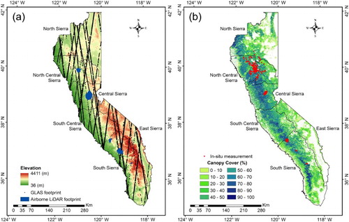
The SN is a mountain range located in the western US, which runs ∼640 km from north to south and ∼110 km from west to east (Figure 1(a)). The elevation increases gradually from the northwest to the southeast, and the mean elevation is over 1500 m; the slope, with a mean of 12°, can reach up to 81°, and is generally higher in the southern SN than in the northern SN. The lower elevation western SN foothills are covered by Mediterranean forests, woodlands and shrub woodlands, and higher elevation mountainous areas are temperate coniferous forests. The region is composed of six sub-regions, namely North Sierra, North Central Sierra, Central Sierra, South Central Sierra, South Sierra, and East Sierra (Figure 1).

Figure 1. (a) The location and elevation of the Sierra Nevada (SN), and the distributions of Geoscience Laser Altimeter System (GLAS) footprints and airborne light detection and ranging (LiDAR) data within the SN. (b) The distributions of canopy cover and in situ measurements within the SN.

2.2. In situ measurements

Field observed tree heights are fundamental for calculating and validating tree height estimations from remotely sensed data. In this study, we collected 1671 plot measurements from SNAMP, Critical Zone Observatory (CZO), and USFS, covering an area of over 6000 km² (Figure 1(b)). All plot measurements from SNAMP and CZO were taken under the same protocol in the growing season of 2012 and 2013. Each plot, 12.62 m in radius (∼500 m² in area), was randomly selected in the corresponding sites of these projects. The height and diameter at breast height (DBH) for each individual tree with a DBH >5 cm were collected in the field. The plot measurements from USFS were taken under the national FIA protocol during the growing season between 2004 and 2009 (Woodall, Monleon-Moscardo, and Forest Inventory 2008). These plots were originally set to study the behaviour of the California spotted owl (Strix occidentalis occidentalis), an endangered wildlife species in the SN. Each plot location was randomly selected and had to be potentially suitable for the owl to nest or forage (Su et al. 2015). Overall, there were 1008 FIA subplot-level plots (7.32 m in radius) collected in this study, and 596 of those plots were within the airborne LiDAR footprint (Table 1). The tree height and DBH for each individual tree with a DBH lager than 12.7 cm were recorded in the field.

Table 1. Collected field tree height measurements and airborne light detection and ranging (LiDAR) data in this study.

	Airborne LiDAR		Field measurements
Data source	Year	Coverage (km^2)	Year	Number of plots within LiDAR footprint	Number of plots outside of LiDAR footprint	Plot size*(m)
SNAMP	2012 and 2013	850	2013	606	0	12.62
CZO	2009	58	2009	57	0	12.62
USFS	2009–2012	676	2004–2009	596	412	7.32

* The size of circular plot is presented by the length of radius.

2.3. Spaceborne LiDAR data and pre-processing

GLAS on-board the NASA ICESat, which was first launched in January 2003 and retired in February 2010, provided global-scale full-waveform LiDAR measurements. Its footprints, in a nominal diameter of 65 m, were spaced at 170 m along tracks and tens of kilometres across tracks (Schutz et al. 2005). In this study, we collected all available GLA01 and GLA06 products between 2003 and 2009 within the SN from the ICESat/GLAS data pool (http://nsidc.org/data/icesat/order.html). The GLA01 product provided the full-waveform measurements, and the GLA06 product provided the geolocation and data quality for each full-waveform record. The GLAS footprint samples within the SN were further filtered to ensure that (1) they were taken under cloud-free conditions; (2) they had no saturation effect; (3) they had high signal to noise ratio (i.e. >50); and (4) they were not significantly higher (i.e. 100 m) than the land surface presented by the Shuttle Radar Topography Mission (SRTM) digital elevation model (DEM). Overall, there are 27,214 GLAS full-waveform samples retained within the SN (Figure 1). For each GLAS sample, we calculated three parameters from the full-waveform information, namely waveform extent, leading edge extent, and trailing edge extent. These three parameters have been proved to be highly correlated to canopy height, canopy height variability, and terrain slope, respectively (Baghdadi et al. 2014; Bourgine and Baghdadi 2005; Lefsky 2010; Lefsky et al. 2007). Definitions of these three parameters can be found in Lefsky et al. (2007), and will not be discussed in detail here.

2.4. Airborne LiDAR data and pre-processing

In this study, the airborne LiDAR data, covering around 1600 km², were collected from the SNAMP, CZO, and USFS (Figure 1). These airborne LiDAR data were all acquired in the growing season during the years of 2009–2013 (Table 1). The average point density for each airborne LiDAR footprint ranges from 4 to 12 pts/m². Within each airborne LiDAR footprint, a 1-m resolution DEM was first interpolated from the LiDAR ground returns using ordinary kriging, since it outperformed other interpolation schemes (e.g. inverse distance weighted and spline) for generating DEM from LiDAR-derived elevation points (Clark, Clark, and Roberts 2004; Guo et al. 2010). Then, the elevation of each LiDAR point was normalised by the obtained DEMs. Finally, canopy quantile metrics, representing the height below X% of the LiDAR point cloud, were generated from these normalised LiDAR point clouds. Canopy quantile metrics are frequently used to compute forest structure parameters that cannot be measured directly from LiDAR point cloud (Lim and Treitz 2004; Thomas et al. 2006). In this study, 11 canopy quantile metrics, including 0%, 1%, 5%, 25%, 50%, 75%, 90%, 95%, 99%, and 100%, were generated for each LiDAR footprint at 20-m resolution, which is roughly correspondent to the plot size.

2.5. Wall-to-wall tree height estimation method

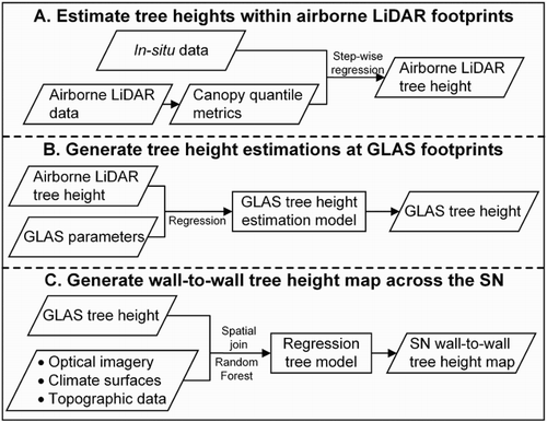
As can be seen in Figure 2, a three-step procedure was used to estimate the wall-to-wall tree height across the SN: (1) estimate tree height within the airborne LiDAR footprint using the step-wise regression method; (2) build regression model to estimate tree heights at GLAS footprints; and (3) extrapolate the tree height estimations from GLAS footprints to the whole SN forests using a regression tree method. It should be noted that tree height mentioned hereafter refers to Lorey’s height (H_L), which can be calculated from in situ individual tree height (H) and basal area (B) measurements,(1) where i is the ith tree within each plot, and n is the total number of tree recorded for each plot.

Figure 2. Flow chart of the proposed SN tree height estimation procedure.

Since the in situ measurements can hardly be spatially coincident with GLAS footprints directly, the airborne LiDAR-derived tree heights were used as the media to link ground measurements with GLAS data (Tang et al. 2014). Previous studies have shown that multiple linear step-wise regression method is an effective method to estimate Lorey’s height from airborne LiDAR canopy quantile metrics and inventory data (Andersen, McGaughey, and Reutebuch 2005; Hall et al. 2005). In this study, within each airborne LiDAR footprint, two-thirds of the corresponding plot measurements were randomly selected, and used as training data to build the regression model for estimating tree height at the airborne LiDAR footprints. These airborne LiDAR-derived tree height estimations were then used to spatially link GLAS measurements, and therefore built a multiple linear regression model to estimate tree height from GLAS parameters (Lefsky et al. 2007). This regression model was applied to all GLAS data to calculate tree heights at GLAS footprints. It should be noted that all airborne LiDAR-derived tree heights were resampled from 20 to 70 m resolution using the weighted mean value method in this step (Jakubowksi et al. 2013) so that they can roughly match the footprint size of GLAS measurements.

The regression tree method random forest (RF) was employed to extrapolate the tree height estimations from GLAS footprints to the whole SN forests. Saatchi et al. (2011) suggested that the normality of co-variables used in the forest parameter prediction models is often violated when complex environmental and ecological parameters are introduced. RF is a formalised non-parametric machine learning algorithm, which does not require the assumption to be made regarding the normality of covariables (Breiman 2001). Moreover, previous studies have shown that the RF algorithm is robust in modelling forest parameters (e.g. tree height and aboveground biomass) from GLAS data and other remotely sensed imagery (Baccini et al. 2008; Simard et al. 2011; Su, Guo, Xue et al. 2016; Wilkes et al. 2015).

In this study, 14 ancillary datasets were included in the RF regression tree model, primarily representing vegetation, climate, and topographic conditions (Table 2). All available Landsat TM Land Surface Reflectance images covering the SN from the growing season of 2009 were collected. These images were further visually examined to make sure the cloud and snow coverage was lower than 10%. The maximum value composite (MVC) was then calculated from those retained Landsat TM images, and the six spectral bands of the MVC (the thermal band was excluded) were used in the RF regression model. In addition, we also computed the normalised vegetation difference index (NDVI) from the MVC and included it in the RF regression tree model. All covariables were interpolated into 70-m resolution using bilinear interpolation method to match the GLAS footprint size. Note that the slope product was generated from the interpolated SRTM DEM product using ESRI^TM ArcMap software.

Table 2. Ancillary datasets used in the random forest regression tree procedure to map forest tree height across the Sierra Nevada.

Dataset	Year	Resolution (m)	Data source
Landsat TM land surface reflectance product	2009	30	US Geological Survey
NDVI calculated from Landsat TM images	2009	30	N/A*
Tree canopy cover	2011	30	National Land Cover Database
Annual mean temperature	1950–2010	70	Alvarez et al. (2014)
Annual temperature seasonality	1950–2010	70	Alvarez et al. (2014)
Annual total precipitation	1950–2010	70	Alvarez et al. (2014)
Annual temperature seasonality	1950–2010	70	Alvarez et al. (2014)
SRTM elevation dataset	2000	30	US Geological Survey
Slope calculated from SRTM data	2000	70	N/A*

* ‘N/A’ represents the corresponding dataset is calculated from other collected dataset.

The RF extrapolation procedure was implemented using the randomForest R package (Liaw and Wiener 2002), which included both the classification and regression functions. There are two primary user defined parameters, number of trees and number of variables tried at each split (Liaw and Wiener 2002). In this study, these two parameters were determined by manual examination. The number of trees and number of variables tried at each split were increased by one iteratively, and the values that produced the minimum mean-squared error were selected to extrapolate the GLAS tree height measurements. Here, based on manual iterative examination, 500 ‘RF trees’ were included and four variables were tried at each split. The built RF regression tree model was used to map the forest tree height across the SN. This initial SN tree height result was further masked by tree canopy cover product to obtain the final SN tree height product (Figure 2). In areas without tree coverage (tree canopy cover = 0%), tree height values were set to 0 m.

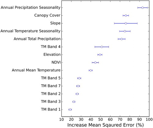
The large amount of covariables used in the extrapolation process may result in the RF algorithm overfitting the model. To reduce this possibility, we further examined the importance of all collected variables, which was evaluated by the percentage increase in the mean-squared error (Liaw and Wiener 2002). The larger the value was, the more important the corresponding variable was. As can be seen in Figure 3, all Landsat TM MVC spectral bands (except band 4) had relatively lower importance to the RF regression model. Therefore, these five bands were not used in the above-mentioned RF regression model.

Figure 3. Importance of variables, denoted by percentage increase of mean-squared error, for the forest tree height estimation random forest model.

2.6. Accuracy assessment

The accuracy of the estimated wall-to-wall SN tree height product was evaluated using the collected plot measurements, airborne LiDAR-derived tree height, and GLAS-derived tree height, respectively. Two commonly used statistical parameters, adjusted coefficient of determination (denoted as R²) and root-mean-squared error (RMSE), were calculated from the following equations,(2) (3) where n is the number of samples, p is the degree of freedom (i.e. number of parameters), x_i is the ith original value, and is the ith estimated value. Moreover, the test statistics was performed on all regression analyses at the significance level (α) of 0.01.

To further evaluate the accuracy of our product, this study collected other available tree height products covering the SN and compared our result with these products. Overall, we found five published works from Simard et al. (2011), Los et al. (2012), Lefsky (2010), Kellndorfer et al. (2012), and Zhang et al. (2014) covering the SN. Simard et al. (2011) estimated the global forest canopy height (RH100) distribution at 1-km resolution from GLAS data, MODIS data, climate surfaces, and topographic data; Los et al. (2012) estimated the forest tree height between 60°N and 60°S by decomposing GLAS waveforms and aggregated them into a spatial continuous layer at 0.5°; Lefsky (2010) segmented the global forests into over 4.4 million patches using MODIS data, and estimated the tree height value for each patch from GLAS data; Kellndorfer et al. (2012) estimated the US nation-wide tree height (Lorey’s height) distribution at 30-m resolution using FIA plot measurements, SRTM data, and three-season Landsat ETM+ data; Zhang et al. (2014) estimated the tree height distribution in California at 30-m resolution using GLAS data and Landsat TM derived leaf area index data. Unfortunately, the tree height products from Lefsky (2010) and Zhang et al. (2014) are not available to us. The data downloading link provided by Lefsky (2010) in the paper is not accessible anymore. Therefore, the current study only compared our result with the products from Simard et al. (2011), Los et al. (2012), and Kellndorfer et al. (2012). To match the spatial resolution of our result and products from Simard et al. (2011) and Los et al. (2012), we resampled our SN tree height map into 1-km resolution and 0.5° resolution respectively by averaging values of all 70-m cells within each coarser resolution cell; to match the spatial resolution with the product from Kellndorfer et al. (2012), we resampled their product into 70-m resolution using a similar procedure.

3. Results

3.1. Tree height estimations within airborne LiDAR footprints

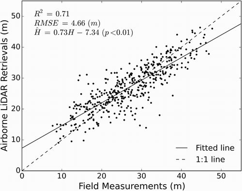
The Lorey’s height distribution within each airborne LiDAR footprint was estimated using the step-wise regression method from corresponding plot measurements and canopy quantile metrics. To evaluate the accuracy of airborne LiDAR-derived tree heights, one-third of the plot measurements within each airborne LiDAR footprint were retained from the regression analysis. Figure 4 shows the accuracy assessment result of airborne LiDAR-derived tree heights using all evaluation plot samples. As can be seen, airborne LiDAR-derived tree heights show good agreements with field measurements. The R² is higher than 0.7 and the RMSE is around 4.7 m. However, it still tends to slightly overestimate the tree heights at areas with low trees, and underestimate tree heights at areas with relatively tall trees (Figure 4).

Figure 4. Evaluation of the airborne LiDAR retrieved Lorey’s height using the validation field measurements. Note that R² represents the adjusted coefficient of determination, RMSE represents the root-mean-square error, H represents the Lorey’s height calculated from field measurements, and represents the airborne LiDAR retrieved Lorey’s height.

3.2. Tree height estimations at GLAS footprints

By linking GLAS parameters with airborne LiDAR-derived tree heights, this study estimated forest tree heights at GLAS footprints using the step-wise regression method. The waveform extent, leading edge extent, trailing edge extent, and slope were used to build the regression model. The following model combining waveform extent, leading edge extent, and trailing edge extents was selected by the step-wise regression method,(4) where LH_GLAS is the estimated Lorey’s height at GLAS footprint, WE is the waveform extent, and LE is the leading edge extent. The R² for the regression model is 0.71, and all coefficients and the constant in the model are statistically significant. This regression model was used to compute tree heights for GLAS footprints outside of airborne LiDAR boundaries.

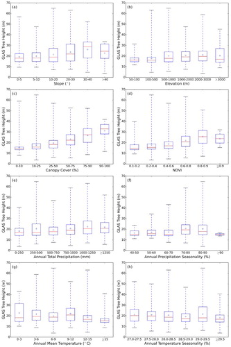
Figure 5 shows the distributions of GLAS estimated tree heights against different topography, vegetation, and climate conditions. As can be seen from Figure 5(a) and (b), topographic parameters (slope and elevation) have similar relationships with GLAS tree heights. The GLAS tree height first increases with both slope and elevation, and then decreases after reaching certain values (40° for slope and 3000 m for elevation respectively). Canopy cover and NDVI share a similar positive influence on GLAS tree heights (Figure 5(c,d)). The higher the canopy cover or NDVI is, the higher the tree height is. There is one exception for the influence of NDVI on GLAS tree height. After NDVI reaches 0.9, the GLAS tree height has a slight decrease compared to previous NDVI group. Annual total precipitation and annual precipitation seasonality have weak positive correlations with GLAS tree heights (Figure 5(e,f)). Once the annual total precipitation reaches 1000 mm or the annual precipitation seasonality reaches 70% (except the group with values larger than 90%), the average GLAS tree height become stable. The exception for the group with an annual precipitation seasonality larger than 90% may be caused by the relatively small number of GLAS footprints within this group (Figure S1). Annual mean temperature is negatively correlated with the GLAS tree height (Figure 5(g)), and annual temperature seasonality has no correlation with the GLAS tree height (Figure 5(h)).

Figure 5. Boxplots of GLAS-derived tree height corresponding to different terrain, vegetation, and climate parameters. The blue ‘+’ indicates the mean GLAS-derived tree height of corresponding group.

3.3. Extrapolated wall-to-wall SN tree height product

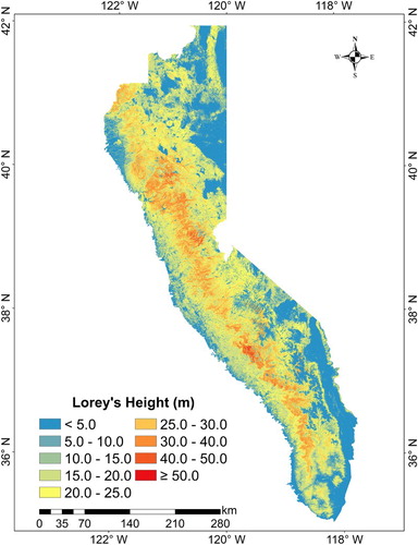
The wall-to-wall 70-m resolution forest tree height map across the SN is shown in Figure 6. Overall, the built RF regression tree model can explain 62.63% of the variation in GLAS tree heights. The average tree height of the whole SN is 14.86 m and the standard deviation is 11.11 m. For forested areas (with a canopy cover larger than 0%), the average tree height is 21.88 m and the standard deviation is 5.32 m.

Figure 6. Estimated forest tree height (Lorey’s height) distribution across the SN.

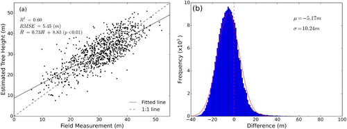
To evaluate the estimated SN tree height product, we compared the obtained product with plot measurements, airborne LiDAR-derived tree height, and GLAS tree height, respectively. As shown in Figure 7(a), the estimated SN tree height product is in good correspondence with field measurements (R² = 0.60, RMSE = 5.45 m). Moreover, although the fitted line is close to the 1:1 line, the estimated SN tree height product tends to overestimate tree heights in areas with relatively low trees (<33 m), and the lower the tree is, the more pronounced the overestimation effect is. In areas with relatively higher trees, the estimated SN tree height product tends to slightly underestimate tree heights. A pixel level comparison between the estimated SN tree height product and the airborne LiDAR-derived tree heights was shown in Figure 7(b). The difference between the estimated tree height and airborne LiDAR-derived tree height follows a normal distribution with a mean of −5.17 m and a standard deviation of 10.24 m. Around 61% of differences between them are within the range of ±10 m, and around 34% of those are within the range of ±5 m. In general, the estimated SN tree height product tends to be lower than the airborne LiDAR-derived tree heights. Around 72% pixels of the airborne LiDAR-derived tree heights are higher than the SN tree height product.

Figure 7. (a) Scatter plot between estimated tree heights () and field measured tree heights (H). (b) Histogram of differences between estimated tree height and airborne LiDAR-derived tree height (estimated tree height minus airborne LiDAR-derived tree height). Note that μ and σ represent the mean and the standard deviation of the differences, respectively.

The accuracy of the modelled SN tree height product was further evaluated by comparing it to GLAS tree heights. Table 3 shows the statistics of differences between the estimated SN tree height product and GLAS tree heights for each sub-region. The differences range approximately between −10 and 10 m (except the North Central Sierra and South Sierra regions), and the average differences for all sub-regions are near 0 m. The standard deviation of differences is lower than 2.4 m for all sub-regions, except the South Sierra region, which is the highest among all sub-regions. Moreover, we further examine the difference between the estimated SN tree height product and GLAS tree heights within 0.25° cells (Figure 8). The model RMSE for each cell was calculated from all footprint level GLAS tree heights within the cell. It should be noted that there were five cells were not covered by any GLAS footprints, and their model RMSE values were interpolated from their neighbouring cells using bilinear interpolation method. As shown in Figure 8, the model RMSE ranges from 0.3 to 15.6 m, and about a half of the 0.25°cells are smaller than 6.5 m. Most of cells with large RMSE values are concentrated in the East Sierra and South Sierra regions.

Figure 8. RMSE of the estimated forest tree height with respect to that calculated from GLAS shots in 0.25° cells.

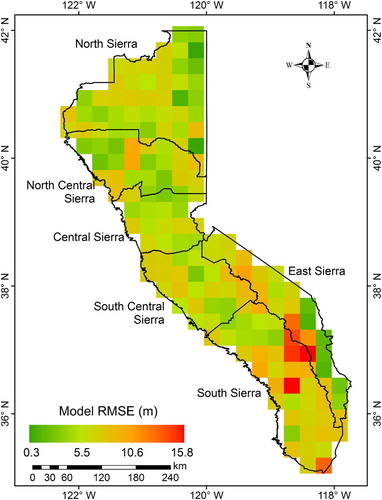
Table 3. Statistics for differences between GLAS-derived tree height and estimated forest tree height products at sub-region scale.

Sub-region	Number of GLAS shots	Minimum (m)	Maximum (m)	Average (m)	Standard deviation (m)
North Sierra	6320	−7.98	10.69	–0.06	1.33
North Central Sierra	4251	−12.63	20.43	–0.10	2.37
Central Sierra	3155	−11.57	11.45	−0.14	2.22
South Central Sierra	4412	−9.09	13.83	–0.07	1.94
South Sierra	5284	−19.47	36.80	0.07	4.03
East Sierra	3792	−8.58	11.16	0.00	1.40

3.4. Comparison with published products

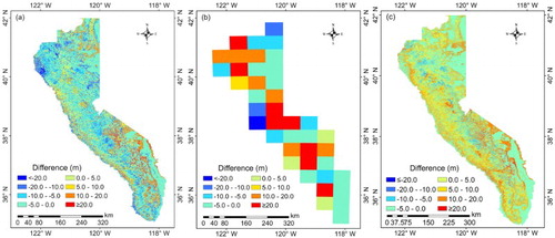
Figure 9 shows the pixel level differences between our estimated SN tree height result and the products from Simard et al. (2011), Los et al. (2012), and Kellndorfer et al. (2012). The mean difference between our result and the product from Simard et al. (2011) is −1.1 m, and the standard deviation is 9.0 m. The differences for over 77% of the 1 km cells are within ±10 m. Due to the coarse resolution of the result from Los et al. (2012), there are only 41 cells within the SN (Figure 9(b)). In general, their result tends be taller than ours in areas with low trees, and be lower than ours in areas with tall trees. The differences for 16 out of the 41 cells are within the range from −5 to 5 m, and over a half are within the range from −10 to 10 m. The tree height product from Kellndorfer et al. (2012) also tends to lower than our product (Figure 9(c)). The mean difference between our product and the product from Kellndorfer et al. (2012) is 3.6 m, and the standard deviation is 7.3 m. Over 81% pixels from our SN tree height product have larger values than the product from Kellndorfer et al. (2012).

Figure 9. Pixel level comparison between our estimated SN tree height product and tree height products from (a) Simard et al. (2011), (b) Los et al. (2012), and (c) Kellndorfer et al. (2012). The pixel level differences are calculated by our SN tree height product minus other products.

4. Discussion

This study developed a procedure to map the fine-resolution tree height distribution across the SN through the combination of ground inventory, airborne LiDAR, and GLAS data. The footprint level GLAS tree heights estimated from GLAS parameters and airborne LiDAR-derived tree heights provided the foundation to build the RF regression tree model, and therefore estimate wall-to-wall tree height distribution from ancillary datasets. As mentioned in Section 3.2, different topographic, vegetation, and climate parameters have different influences on the SN tree height distribution (Figure 5). With the increase of both slope and elevation, the GLAS tree height increases first and then decrease after they reach to certain thresholds (Figure 5(a,b)). This may be caused by the tree species distribution pattern in the SN. The SN oak woodlands are generally distributed in foothill areas with low elevation (<1200 m) and slope values, and the height of oak trees are usually lower than 15 m; pine forests and mixed conifer forest mainly spread out in areas with steep slope and elevation from 1200 m to around 2200 m, and individual tree height is usually taller than 15 m; in areas with elevation higher than ∼2300 m, the conditions for tree growth become harsher and the main vegetation group is upper montane forest (Barbour and Billings 2000). Similar to previous studies, we found that NDVI had saturation effect when being used to model forest canopy parameters, because of the limited penetration capability of optical sensors (Lu 2006; Lu et al. 2004; Wang et al. 2005). Moreover, both the annual total precipitation and annual precipitation seasonality have a positive influence on the SN tree height, but the influence may become saturated when values reach certain thresholds. The exception for the group with an annual precipitation seasonality higher than 90% may be caused by the fact that too few GLAS footprints fall in this group. Annual mean temperature has a unique negative correlation with the SN tree height. This may be caused by the reason that the temperature decreases with the increase of elevation, and most tall coniferous trees are distributed in relatively high elevation areas in the SN (Barbour and Billings 2000).

Although our SN tree height product shows good spatial correspondence with the other three published products, there are still differences. In general, our result shows more variations in tree height than the product from Simard et al. (2011). In areas with relatively steeper slopes (>15°), tree height from our result tends to be taller than that from Simard et al. (2011). One possible reason for this is that they did not include terrain slope in their tree height mapping procedure, and the GLAS waveform parameters are highly influenced by the terrain slope (Lefsky et al. 2007). Along the eastern foothills of the SN, our result also tends to be higher than the tree height from Simard et al. (2011) (Figure 9(a)). Moreover, although both our SN tree height product and the product from Kellndorfer et al. (2012) are Lorey’s height, our tree height product is systematically higher. This may be caused by the fact that Kellndorfer et al. (2012) only used the Landsat ETM+ data and SRTM data to map the forest tree height. As mentioned, model-based tree height measurements from optical sensors are usually suffered from the saturation effects, especially in areas with high values (Donoghue and Watt 2006; McCombs, Roberts, and Evans 2003; Su et al. 2015).

Several issues may have complicated the comparison analysis in this study. First of all, the definition of tree height among these three products is different. The tree height mentioned in this study refers to the Lorey’s height. However, the tree height from Simard et al. (2011) is defined by the GLAS waveform shape parameter RH100, and that from Los et al. (2012) is calculated by decomposing the GLAS waveform, which are both expected to be higher than Lorey’s height. This may be also one of the reasons that the differences for around 60% of the 1 km cells between our product and the product from Simard et al. (2011) are negative. Moreover, the spatial resolution of these three products is significantly different. The resampling process may further increase the uncertainty in the comparison results.

The accuracy of the estimated SN tree height product was evaluated by ground plot measurements, airborne LiDAR-derived tree heights, and footprint level GLAS tree heights, respectively. These accuracy assessment results indicate that our SN tree height product can be used to reflect the spatial distribution of canopy height in the SN. Although the RMSE of the product is around 5.5 m by comparing with ground measurements, and may even reach over 10 m by comparing with airborne LiDAR tree height at pixel level, the map from this study provides one of the best options to understand and explore forest tree height variation across the SN at fine resolution. However, this study still has limitations. Firstly, the time span of the data used in this study is very wide. The GLAS data were acquired between 2003 and 2009, and the airborne LiDAR data and ground measurements were taken from 2004 to 2013. Wensel, Meerschaert, and Biging (1987) found that without human interference, the conifer trees in the northern California can increase around 3–5 m every five years. Therefore, the influence of tree growth during the time span of airborne LiDAR data and in situ measurements cannot be neglected. Moreover, forest changes brought by both nature incidents (e.g. wildfires) and human activities (e.g. forest fuel treatment, deforestation, and reforestation) may also result in significant changes in tree heights (Su, Guo, Collions et al. 2016). Secondly, the current accuracy assessment using independent plot measurements may be biased due to the mismatch between the plot size and the cell size of the estimated product. In the current study, we do not have access to in situ measurements with bigger plot size, and we cannot produce the tree height map with finer resolution due to the limitation of the GLAS plot size. This issue can be addressed by collecting more airborne LiDAR data in the SN. With enough airborne LiDAR data, we can directly derive the tree height without using GLAS data, which allows us to map the SN tree height with finer (30 m) resolution. Finally, this study has not performed a fine-resolution uncertainty analysis on the obtained result using error propagation method. Future study is still needed to analyse how the uncertainty from different prediction variables influence the tree height estimation result.

5. Conclusions

This study presented a method to map fine-resolution forest tree height across the SN by combining plot measurements, airborne LiDAR data, GLAS data, optical imagery, topographic data, and climate surfaces. Over 1600 in situ field measurements and airborne LiDAR data covering around 1600 km² were collected to address this mission. The resulting SN tree height map at 70-m resolution is available at the web (http://guolablidar.com/SNtreeheight). Across the SN, the average tree height is 14.86 m and the standard deviation is 11.11 m; for only forested areas, the average tree height is 21.88 m and the standard deviation is 5.32 m. The estimated SN tree height product shows good agreements with in situ plot measurements (R² = 0.60, RMSE = 5.45 m). The mean difference between the estimated SN tree height product and airborne LiDAR-derived tree heights is −5.17 m, and the estimated product tends to be lower than airborne LiDAR-derived tree heights. This fine-resolution SN tree height map can be used to reveal the canopy vertical structure characteristics of the SN forests.

Acknowledgements

We thank Dr John J. Keane, Dr Ross A. Gerrard, and Claire V. Gallagher for providing valuable suggestions on the development of tree height estimation algorithm in this study.

Disclosure statement

No potential conflict of interest was reported by the authors.

ORCiD

Yanjun Su http://orcid.org/0000-0001-7931-339X

Qin Ma http://orcid.org/0000-0002-6995-6663

Qinghua Guo http://orcid.org/0000-0002-9589-6078

Additional information

Funding

This study is supported by the National Science Foundation of China [project numbers 41471363 and 31270563], National Science Foundation [DBI 1356077], and the USDA Forest Service Pacific Southwest Research Station.

References

- Alvarez, Otto, Qinghua Guo, Robert C. Klinger, Wenkai Li, and Paul Doherty. 2014. “Comparison of Elevation and Remote Sensing Derived Products as Auxiliary Data for Climate Surface Interpolation.” International Journal of Climatology 34 (7): 2258–2268. doi: 10.1002/joc.3835
- Andersen, Hans-Erik, Robert J. McGaughey, and Stephen E. Reutebuch. 2005. “Estimating Forest Canopy Fuel Parameters Using LIDAR Data.” Remote Sensing of Environment 94 (4): 441–449. doi: 10.1016/j.rse.2004.10.013
- Andersen, Hans-Erik, Stephen E. Reutebuch, and Robert J. McGaughey. 2006. “A Rigorous Assessment of Tree Height Measurements Obtained Using Airborne Lidar and Conventional Field Methods.” Canadian Journal of Remote Sensing 32 (5): 355–366. doi: 10.5589/m06-030
- Baccini, A., N. Laporte, S. J. Goetz, M. Sun, and H. Dong. 2008. “A First Map of Tropical Africa’s Above-ground Biomass Derived from Satellite Imagery.” Environmental Research Letters 3 (4): 045011. doi: 10.1088/1748-9326/3/4/045011
- Baghdadi, Nicolas, Guerric Le Maire, Ibrahim Fayad, JeanStéphane Bailly, Yann Nouvellon, Cristiane Lemos, and Rodrigo Hakamada. 2014. “Testing Different Methods of Forest Height and Aboveground Biomass Estimations from ICESat/GLAS Data in Eucalyptus Plantations in Brazil.” IEEE Journal of Selected Topics in Applied Earth Observations and Remote Sensing 7 (1): 290–299. doi: 10.1109/JSTARS.2013.2261978
- Bales, Roger C., John J. Battles, Yihsu Chen, Martha H. Conklin, Eric Holst, Kevin L. O’Hara, Philip Saksa, and William Stewart. 2011. “Forests and Water in the Sierra Nevada: Sierra Nevada Watershed Ecosystem Enhancement Project.” In Sierra Nevada Research Institute report, 2–5. Merced, CA: Sierra Nevada Research Institute.
- Barbour, Michael G., and William Dwight Billings. 2000. North American Terrestrial Vegetation. Cambridge: Cambridge University Press.
- Berigan, William J, R. J. Gutiérrez, and Douglas J. Tempel. 2012. “Evaluating the Efficacy of Protected Habitat Areas for the California Spotted Owl Using Long-term Monitoring Data.” Journal of Forestry 110 (6): 299–303. doi: 10.5849/jof.11-018
- Bourgine, Bernard, and Nicolas Baghdadi. 2005. “Assessment of C-band SRTM DEM in a Dense Equatorial Forest Zone.” Comptes Rendus Geoscience 337 (14): 1225–1234. doi: 10.1016/j.crte.2005.06.006
- Breiman, Leo. 2001. “Random Forests.” Machine learning 45 (1): 5–32. doi: 10.1023/A:1010933404324
- Clark, Matthew L., David B. Clark, and Dar A. Roberts. 2004. “Small-footprint LiDAR Estimation of Sub-canopy Elevation and Tree Height in a Tropical Rain Forest Landscape.” Remote Sensing of Environment 91 (1): 68–89. doi: 10.1016/j.rse.2004.02.008
- Coops, Nicholas C., Thomas Hilker, Michael A. Wulder, Benoît St-Onge, Glenn Newnham, Anders Siggins, and J. A. Tony Trofymow. 2007. “Estimating Canopy Structure of Douglas-fir Forest Stands from Discrete-return LiDAR.” Trees 21 (3): 295–310. doi: 10.1007/s00468-006-0119-6
- Donoghue, D. N. M., and P. J. Watt. 2006. “Using LiDAR to Compare Forest Height Estimates from IKONOS and Landsat ETM+ data in Sitka Spruce Plantation Forests.” International Journal of Remote Sensing 27 (11): 2161–2175. doi: 10.1080/01431160500396493
- Duncanson, L. I., K. O. Niemann, and M. A. Wulder. 2010. “Estimating Forest Canopy Height and Terrain Relief from GLAS Waveform Metrics.” Remote Sensing of Environment 114 (1): 138–154. doi: 10.1016/j.rse.2009.08.018
- Guo, Qinghua, Wenkai Li, Hong Yu, and Otto Alvarez. 2010. “Effects of Topographic Variability and Lidar Sampling Density on Several DEM Interpolation Methods.” Photogrammetric Engineering and Remote Sensing 76 (6): 701–712. doi: 10.14358/PERS.76.6.701
- Hall, S. A., I. C. Burke, D. O. Box, M. R. Kaufmann, and J. M. Stoker. 2005. “Estimating Stand Structure Using Discrete-return LiDAR: An Example from Low Density, Fire Prone Ponderosa Pine Forests.” Forest Ecology and Management 208 (1): 189–209. doi: 10.1016/j.foreco.2004.12.001
- Hall, R. J., R. S. Skakun, E. J. Arsenault, and B. S. Case. 2006. “Modeling Forest Stand Structure Attributes Using Landsat ETM+ Data: Application to Mapping of Aboveground Biomass and Stand Volume.” Forest Ecology and Management 225 (1): 378–390. doi: 10.1016/j.foreco.2006.01.014
- Jakubowksi, Marek K., Qinghua Guo, Brandon Collins, Scott Stephens, and Maggi Kelly. 2013. “Predicting Surface Fuel Models and Fuel Metrics Using Lidar and CIR Imagery in a Dense, Mountainous Forest.” Photogrammetric Engineering & Remote Sensing 79 (1): 37–49. doi: 10.14358/PERS.79.1.37
- Kellndorfer, J., W. Walker, E. LaPoint, J. Bishop, T. Cormier, G. Fiske, M. Hoppus, K. Kirsch, and J. Westfall. 2012. “NACP Aboveground Biomass and Carbon Baseline Data (NBCD 2000), U.S.A., 2000: Dataset 2012.” ORNL DAAC, Oak Ridge, Tennessee. http://daac.ornl.gov.
- Leckie, Don, François Gougeon, David Hill, Rick Quinn, Lynne Armstrong, and Roger Shreenan. 2003. “Combined High-density Lidar and Multispectral Imagery for Individual Tree Crown Analysis.” Canadian Journal of Remote Sensing 29 (5): 633–649. doi: 10.5589/m03-024
- Lefsky, Michael A. 2010. “A Global Forest Canopy Height Map from the Moderate Resolution Imaging Spectroradiometer and the Geoscience Laser Altimeter System.” Geophysical Research Letters 37 (15): L15401. doi: 10.1029/2010GL043622
- Lefsky, Michael A., David J. Harding, Michael Keller, Warren B. Cohen, Claudia C. Carabajal, Fernando Del Bom Espirito-Santo, Maria O. Hunter, and Raimundo de Oliveira. 2005. “Estimates of Forest Canopy Height and Aboveground Biomass Using ICESat.” Geophysical Research Letters 32 (22): L22S02. doi: 10.1029/2005GL023971
- Lefsky, Michael A., Michael Keller, Yong Pang, Plinio B. De Camargo, and Maria O. Hunter. 2007. “Revised Method for Forest Canopy Height Estimation from Geoscience Laser Altimeter System Waveforms.” Journal of Applied Remote Sensing 1 (1): 013537. doi: 10.1117/1.2795724
- Liaw, Andy, and Matthew Wiener. 2002. “Classification and Regression by RandomForest.” R News 2 (3): 18–22.
- Lim, Kevin S., and Paul M. Treitz. 2004. “Estimation of Above Ground Forest Biomass from Airborne Discrete Return Laser Scanner Data Using Canopy-based Quantile Estimators.” Scandinavian Journal of Forest Research 19 (6): 558–570. doi: 10.1080/02827580410019490
- Los, S. O., J. A. B. Rosette, Natascha Kljun, P. R. J. North, Laura Chasmer, J. C. Suárez, Chris Hopkinson, et al. 2012. “Vegetation Height and Cover Fraction Between 60 S and 60 N from ICESat GLAS Data.” Geoscientific Model Development 5 (2): 413–432. doi: 10.5194/gmd-5-413-2012
- Lu, Dengsheng. 2006. “The Potential and Challenge of Remote Sensing-based Biomass Estimation.” International Journal of Remote Sensing 27 (7): 1297–1328. doi: 10.1080/01431160500486732
- Lu, Dengsheng, Paul Mausel, Eduardo Brondızio, and Emilio Moran. 2004. “Relationships Between Forest Stand Parameters and Landsat TM Spectral Responses in the Brazilian Amazon Basin.” Forest Ecology and Management 198 (1): 149–167. doi: 10.1016/j.foreco.2004.03.048
- Martinuzzi, Sebastián, Lee A. Vierling, William A. Gould, Michael J. Falkowski, Jeffrey S. Evans, Andrew T. Hudak, and Kerri T. Vierling. 2009. “Mapping Snags and Understory Shrubs for a LiDAR-based Assessment of Wildlife Habitat Suitability.” Remote Sensing of Environment 113 (12): 2533–2546. doi: 10.1016/j.rse.2009.07.002
- Matthews, Sean M., J. Mark Higley, John T. Finn, Kerry M. Rennie, Craig M. Thompson, Kathryn L. Purcell, Rick. A Sweitzer, Sandra L. Haire, Paul R. Sievert, and Todd K. Fuller. 2013. “An Evaluation of a Weaning Index for Wild Fishers (Pekania [Martes] pennanti) in California.” Journal of Mammalogy 94 (5): 1161–1168. doi: 10.1644/12-MAMM-A-249.1
- McCombs, John W., Scott D. Roberts, and David L. Evans. 2003. “Influence of Fusing Lidar and Multispectral Imagery on Remotely Sensed Estimates of Stand Density and Mean Tree Height in a Managed Loblolly Pine Plantation.” Forest Science 49 (3): 457–466.
- Morsdorf, Felix, Benjamin Kötz, Erich Meier, K. I. Itten, and Britta Allgöwer. 2006. “Estimation of LAI and Fractional Cover from Small Footprint Airborne Laser Scanning Data Based on Gap Fraction.” Remote Sensing of Environment 104 (1): 50–61. doi: 10.1016/j.rse.2006.04.019
- Naesset, Erik. 1997. “Determination of Mean Tree Height of Forest Stands Using Airborne Laser Scanner Data.” ISPRS Journal of Photogrammetry and Remote Sensing 52 (2): 49–56. doi: 10.1016/S0924-2716(97)83000-6
- Næsset, Erik, and Tonje Økland. 2002. “Estimating Tree Height and Tree Crown Properties Using Airborne Scanning Laser in a Boreal Nature Reserve.” Remote Sensing of Environment 79 (1): 105–115. doi: 10.1016/S0034-4257(01)00243-7
- Nelson, Ross, William Krabill, and Gordon MacLean. 1984. “Determining Forest Canopy Characteristics Using Airborne Laser Data.” Remote Sensing of Environment 15 (3): 201–212. doi: 10.1016/0034-4257(84)90031-2
- Nilsson, Mats. 1996. “Estimation of Tree Heights and Stand Volume Using an Airborne Lidar System.” Remote Sensing of Environment 56 (1): 1–7. doi: 10.1016/0034-4257(95)00224-3
- Popescu, Sorin C., Randolph H. Wynne, and Ross F. Nelson. 2002. “Estimating Plot-level Tree Heights with Lidar: Local Filtering with a Canopy-height Based Variable Window Size.” Computers and Electronics in Agriculture 37 (1): 71–95. doi: 10.1016/S0168-1699(02)00121-7
- Popescu, Sorin C., Kaiguang Zhao, Amy Neuenschwander, and Chinsu Lin. 2011. “Satellite Lidar vs. Small Footprint Airborne Lidar: Comparing the Accuracy of Aboveground Biomass Estimates and Forest Structure Metrics at Footprint Level.” Remote Sensing of Environment 115 (11): 2786–2797. doi: 10.1016/j.rse.2011.01.026
- Saatchi, Sassan S., Nancy L. Harris, Sandra Brown, Michael Lefsky, Edward TA Mitchard, William Salas, Brian R. Zutta, et al. 2011. “Benchmark Map of Forest Carbon Stocks in Tropical Regions Across three Continents.” Proceedings of the National Academy of Sciences, 108 (24): 9899–9904. doi: 10.1073/pnas.1019576108
- Schutz, B. E., H. J. Zwally, C. A. Shuman, D. Hancock, and J. P. DiMarzio. 2005. “Overview of the ICESat Mission.” Geophysical Research Letters 32 (21): L21S01. doi: 10.1029/2005GL024009
- Simard, Marc, Naiara Pinto, Joshua B. Fisher, and Alessandro Baccini. 2011. “Mapping Forest Canopy Height Globally with Spaceborne Lidar.” Journal of Geophysical Research: Biogeosciences (2005–2012) 116 (G4): G04021. doi: 10.1029/2011JG001708
- Stephens, Scott L., ConstanceI Millar, and Brandon M. Collins. 2010. “Operational Approaches to Managing Forests of the Future in Mediterranean Regions within a Context of Changing Climates.” Environmental Research Letters 5 (2): 024003. doi: 10.1088/1748-9326/5/2/024003
- Su, Yanjun, and Qinghua Guo. 2014. “A Practical Method for SRTM DEM Correction Over Vegetated Mountain Areas.” ISPRS Journal of Photogrammetry and Remote Sensing 87: 216–228. doi: 10.1016/j.isprsjprs.2013.11.009
- Su, Yanjun, Qinghua Guo, Brandon M. Collions, Danny L. Fry, Tianyu Hu, and Maggi Kelly. 2016. “Forest Fuel Treatment Detection Using Multi-temporal Airborne Lidar Data and High-resolution Aerial Imagery: A Case Study in the Sierra Nevada Mountains, California.” International Journal of Remote Sensing 37 (14): 3322–3345. doi: 10.1080/01431161.2016.1196842
- Su, Yanjun, Qinghua Guo, Qin Ma, and Wenkai Li. 2015. “SRTM DEM Correction in Vegetated Mountain Areas through the Integration of Spaceborne LiDAR, Airborne LiDAR, and Optical Imagery.” Remote Sensing 7 (9): 11202–11225. doi: 10.3390/rs70911202
- Su, Yanjun, Qinghua Guo, Baolin Xue, Tianyu Hu, Otto Alvarez, Sshengli Tao, and Jingyun Fang. 2016. “Spatial Distribution of Forest Aboveground Biomass in China: Estimation Through Combination of Spaceborne Lidar, Optical Imagery, and Forest Inventory Data.” Remote Sensing of Environment 173 (2): 187–199. doi: 10.1016/j.rse.2015.12.002
- Suárez, Juan C., Carlos Ontiveros, Steve Smith, and Stewart Snape. 2005. “Use of Airborne LiDAR and Aerial Photography in the Estimation of Individual Tree Heights in Forestry.” Computers & Geosciences 31 (2): 253–262. doi: 10.1016/j.cageo.2004.09.015
- Tang, Hao, Matthew Brolly, Feng Zhao, Alan H. Strahler, Crystal L. Schaaf, Sangram Ganguly, Gong Zhang, and Ralph Dubayah. 2014. “Deriving and Validating Leaf Area Index (LAI) at Multiple Spatial Scales Through Lidar Remote Sensing: A Case Study in Sierra National Forest, CA.” Remote Sensing of Environment 143 (3): 131–141. doi: 10.1016/j.rse.2013.12.007
- Thomas, V., P. Treitz, J. H. McCaughey, and I. Morrison. 2006. “Mapping Stand-level Forest Biophysical Variables for a Mixedwood Boreal Forest Using Lidar: An Examination of Scanning Density.” Canadian Journal of Forest Research 36 (1): 34–47. doi: 10.1139/x05-230
- Vierling, Kerri T., Lee A. Vierling, William A. Gould, Sebastian Martinuzzi, and Rick M. Clawges. 2008. “Lidar: Shedding New Light on Habitat Characterization and Modeling.” Frontiers in Ecology and the Environment 6 (2): 90–98. doi: 10.1890/070001
- Wang, Quan, Samuel Adiku, John Tenhunen, and André Granier. 2005. “On the Relationship of NDVI with Leaf Area Index in a Deciduous Forest Site.” Remote Sensing of Environment 94 (2): 244–255. doi: 10.1016/j.rse.2004.10.006
- Wensel, Lee C., Walter J. Meerschaert, and Greg S. Biging. 1987. “Tree Height and Diameter Growth Models for Northern California Conifers.” Hilgardia 55 (8): 1–20.
- Wilkes, Phil, Simon Jones, Lola Suarez, Andrew Mellor, William Woodgate, Mariela Soto-Berelov, Andrew Haywood, and Andrew Skidmore. 2015. “Mapping Forest Canopy Height Across Large Areas by Upscaling ALS Estimates with Freely Available Satellite Data.” Remote Sensing 7 (9): 12563. doi: 10.3390/rs70912563
- Wing, Brian M., Martin W. Ritchie, Kevin Boston, Warren B. Cohen, and Michael J. Olsen. 2015. “Individual Snag Detection Using Neighborhood Attribute Filtered Airborne Lidar Data.” Remote Sensing of Environment 163: 165–179. doi: 10.1016/j.rse.2015.03.013
- Woodall, Christopher, Vicente J. Monleon-Moscardo, and Forest Inventory. 2008. “Sampling Protocol, Estimation, and Analysis Procedures for the Down Woody Materials Indicator of the FIA Program.”
- Zhang, Gong, Sangram Ganguly, Ramakrishna R. Nemani, Michael A. White, Cristina Milesi, Hirofumi Hashimoto, Weile Wang, Sassan Saatchi, Yifan Yu, and Ranga B. Myneni. 2014. “Estimation of Forest Aboveground Biomass in California Using Canopy Height and Leaf Area Index Estimated from Satellite Data.” Remote Sensing of Environment 151: 44–56. doi: 10.1016/j.rse.2014.01.025
- Zhao, Feng, Qinghua Guo, and Maggi Kelly. 2012. “Allometric Equation Choice Impacts Lidar-based Forest Biomass Estimates: A Case Study from the Sierra National Forest, CA.” Agricultural and Forest Meteorology 165: 64–72. doi: 10.1016/j.agrformet.2012.05.019
- Zhao, Kaiguang, and Sorin Popescu. 2009. “Lidar-based Mapping of Leaf Area Index and its Use for Validating GLOBCARBON Satellite LAI Product in a Temperate Forest of the Southern USA.” Remote Sensing of Environment 113 (8): 1628–1645. doi: 10.1016/j.rse.2009.03.006