Upscaling in situ albedo for validation of coarse scale albedo product over heterogeneous surfaces

ABSTRACT

One of the essential steps for satellite albedo validation is upscaling in situ measurements to corresponding pixel scale over relatively heterogeneous land surfaces. Although the multi-scale validation strategy is applicable for heterogeneous surfaces, the calibration of the high-resolution imagery during upscaling process is never perfect, and thus the upscaling results suffer from errors. The regression-kriging (RK) technique can compensate the calibration part by applying kriging to upscale residuals and produce more accurate upscaling results. In this paper, in situ measurements and high spatial resolution albedo imagery combined with RK technique was proposed. This method is illustrated by upscaling surface albedo from in situ measurements scale to the coarse pixel scale in the core experimental area of HiWATER, where 17 WSN nodes were deployed at heterogeneous area. The upscaling results of this method were compared with the upscaling results from multi-scale strategy. The results show that the upscaling method based on in situ measurements and high-resolution imagery combined with RK technique can capture the spatial characteristics of surface albedo better. Further, an attempt was made to expand this method in time series. Finally, a preliminary validation of the Moderate Resolution Imaging Spectroradiometer albedo product was performed as the tentative application.

KEYWORDS:

• Upscaling
• albedo
• heterogeneous
• validation
• in situ
• multi-scale

1. Introduction

Land surface shortwave albedo (0.3–3 µm) is defined as the ratio of the upwelling shortwave radiation relative to the downwelling shortwave radiation of a land surface (Pinty and Verstraete 1994; Stroeve et al. 2005). It determines the amount of solar radiation absorbed by the land surface (de Souza et al. 2006; Dickinson 1995; Liang 2003; Liu, Yang et al. 2009; Wen et al. 2009). The long-term land surface albedo temporal–spatial distribution can improve our understanding of earth terrestrial energy flux and global environmental change (Valero and Charlson 2008; Zhang, Liang et al. 2010). Thus it is a key input parameter in climate and biogeochemical models. Although remote sensing satellite is the most practical method to estimate consistent albedo because of its large spatial scale and coverage (Liang 2001, 2005), remote sensing retrievals may suffer from large uncertainties due to the inherent complexity of physical processes and their parameterization (Li 2014). These uncertainties will further deviate the result of model simulation and remote sensing applications.

Thus, it is critical to evaluate such satellite-derived albedo products with in situ albedo (Cescatti et al. 2012; Jin et al. 2003, 2012; Qu, Zhu, et al. 2014; Salomon et al. 2006; Schaaf, Wang, and Strahler 2011; Susaki et al. 2007) in order to get their precisions, which is defined as validation. Currently, albedo validation is focused on the places with homogeneous surfaces, where the in situ albedo was considered with high spatial representativeness and can be directly used to validate coarse-scale albedo product. Unfortunately, the land surface albedo is decided by underlying surface status and the homogeneity is relative. We should also evaluate the albedo in heterogeneous land surfaces, where the surface albedo is affected by the spatial scales.

The footprint of in situ observation is limited and it cannot represent the surface albedo at coarse scale in most cases. The direct comparison between in situ value and coarse-pixel albedo products is invalided and will introduce large uncertainty to the validation results if the in situ measurements cannot represent coarse-scale albedo. Hence, upscaling the in situ measurements to the coarse pixel scale became an important step for the validation.

The simplest way to upscale is to aggregate multi-point data over larger areas by averaging the reflectance/albedo of these points. However, the upscaling result highly depends on the spatial representativeness of these points to the surrounding landscapes in the satellite footprint (Wu et al. 2014). Another method is called as ‘multi-scale validation strategy’ that uses high spatial resolution albedo imagery, for example, Enhanced Thematic Mapper (ETM+) or HJ albedo, as an upscaling bridge to reduce the scale discrepancy between in situ observations and coarse-scale satellite observations (Jiao et al. 2005; Liang et al. 2002; Peng, Liu, Wen, et al. 2015; Zhang, Tian et al. 2010). In situ measurements were used to calibrate high-resolution albedo products. Then, the calibrated high-resolution albedo maps were resampled (i.e. upscaled) to assess the accuracy of the coarse resolution albedo products. If the high-resolution albedo imagery is accurate enough or its calibration is perfect, there should be less bias between the upscaling results and the ‘truth’ value of pixel scale albedo. However, it is challenging to obtain sufficiently accurate high-resolution albedo imageries because of the low update limitations, radiometric calibrations, geometric mismatches, atmospheric corrections, and retrieval algorithms. Further, building such an ideal calibration model over heterogeneous surfaces is unrealistic, because the relationship between in situ values and high-resolution albedo values is established based on the individual pixels corresponding to the limited in situ observations. When applying the relationship to other pixels, it will introduce errors. Thus, the upscaled high-resolution albedo may suffer from uncertainty.

In recent years, one promising approach for upscaling over heterogeneous land surface is the regression-kriging (RK)-based technique, which has been used for inferring soil moisture and sensible heat fluxes (Crow et al. 2012; Ge et al. 2015; Kang, Jin, and Li 2015). The RK technique can compensate the residuals that derived from the calibration process by applying kriging to upscale residuals and extend the general multi-point upscaling process by incorporating fine spatial resolution information by regression modeling.

The RK technique can divide the albedo over heterogeneous surface into heterogeneous component, which is conceptualized as the trend surface, and the random component, which is conceptualized as residuals. The trend surface is established by applying a regression approach between environmental variables in the form of imagery and in situ albedo values. The residuals can be derived after removing the trend surface from surface albedo. By considering the spatial autocorrelations of residuals, the residuals can be directly upscaled to coarse scale with a known prediction error variance. In particular, the residuals are more realistic to satisfy the assumption of stationarity of kriging and this technique could produce more accurate predictions over heterogeneous land surfaces (Hengl, Heuvelink, and Rossiter 2007).

This paper proposed an upscaling method based on in situ measurements and high-resolution imagery combined with RK technique, focused on the scaling conversions of ground albedo observations, particularly upscaling from in situ measurements scale to the coarse pixel scale over heterogeneous land surface. This method is applied to the Heihe Watershed Allied Telemetry Experimental Research (HiWATER) experiment. The accuracies of MCD43A3 (V006) values were assessed as the tentative application for upscaling predictions from in situ support resolution to coarse pixel resolution.

This paper is organized as follows: Firstly, the study area and data are described in Section 2. Secondly, details about the upscaling method are outlined in Section 3. In Section 4, the results are presented and discussed. Finally, a brief conclusion is given in Section 5.

2. Data-sets

2.1. Study area and WSN observation

The study area (Figure 1) is located in the middle reach of the Heihe River Basin, which was selected as an experimental watershed for conducting the HiWATER because it is a typical inland river basin that has long served as a test region for integrated watershed studies as well as land surface and hydrologic experiments (Cheng et al. 2014; Li et al. 2013) HiWATER is an ongoing, watershed scale, eco-hydrological experiment designed from an interdisciplinary perspective to address complex problems, such as heterogeneity, scaling, uncertainty, and closing the water cycle at the watershed scale (Li et al. 2013).

Figure 1. The map (Project: WGS_1984_UTM_Zone_47N) of the study area and the distribution of the WSN nodes.

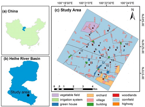
The core experimental area is approximately 5.5 km by 5.5 km, located between 38°50′-38°54′ N and 100°19′-100°24′ E. The main crop in the study region is corn, which covers approximately 75% of the total area. Other plants, including wheat, vegetable, and orchards, are also present. Additionally, the land cover types include buildings, roads, greenhouses, and irrigation channels. The subsurface heterogeneity is the main factor that causes the spatial heterogeneity of the surface albedo. In addition, due to the different types of crop management (i.e. irrigation, fertilization, etc.), even the croplands with the same or different species present different albedo values in different locations. The spatial distribution of the wireless sensor network (WSN) nodes is shown in Figure 1(c). There are 17 in situ WSN measurement nodes installed within the study area and each WSN node is a field site. For each specific coarse-scale pixel, there is no more than one field site.

Seventeen field sites were instrumented with Kipp and Zonen Radiometers measured the total downward and upward shortwave radiation (300–2800 nm), and the in situ albedo was calculated based on their ratios. The radiometers have been strictly calibrated to reduce the measurement uncertainties (Xu et al. 2013). Radiometers were mounted 3 m above the cropland with a footprint of approximately 26 m in diameter (Sailor, Resh, and Segura 2006). The WSN data had a high temporal resolution of 10 min, and the ground-based albedo observations could be precisely synchronized with satellite and airborne remote sensing data. The radiation measurements at local noon on 29 June and 8 July 2012, when high-resolution imagery was acquired, were used to calculate the actual albedo for illustration of the method. In addition, the actual albedo around these 2 days were also calculated for time series expansion purpose.

2.2. Airborne experiment and CASI albedo

The airborne hyperspectral data-sets of compact airborne spectrographic imager (CASI) were simultaneously acquired on 29 June and 8 July 2012, at an altitude of 2500 m (Xiao and Wen 2012) to improve the remote sensing methods used for observing key eco-hydrological processes (Li et al. 2013). CASI1500 is a visible and near-infrared pushbroom hyperspectral sensor (Colgan et al. 2012; Feingersh, Ben-Dor, and Filin 2010). Table 1 shows the basic specifications of CASI sensor. The raw data were acquired as 14-bit digital values and converted into 16-bit radiances (Fan et al. 2015). The CASI image data had been radiometrically calibrated and geometrically corrected to a standard earth-centered coordinate system, which was re-sampled at a resolution of 5 m using a UTM projection. With atmospheric parameters measured from the ground, the Second Simulation of the Satellite Signal in the Solar Spectrum (6S) (Vermote et al. 1997) atmospheric model was adopted to drive the atmospheric parameters that allowed the CASI atmospheric effects to be corrected to obtain the CASI bidirectional function factor at the surface. Preliminary validation of the atmosphere corrected CASI reflectance showed that the absolute differences were 1.5% (relative difference 5.93%) in the visible range of the spectrum (400–700 nm) and 2.5% (relative difference 7.89%) in the near-infrared (700–1055 nm), compared with the reflectance of a homogenous concrete surface measured synchronically in the ground campaign (You et al. 2015).

Table 1. Basic specifications of CASI imagery.

Basic specifications	CASI1500
Spectral range	380–1050 nm
Spatial resolution	1 m
Bands	48
Band width	7 nm
Digitization	14-bit

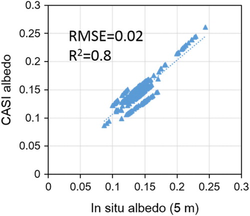
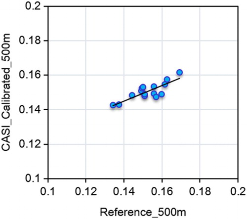
The CASI albedo values were estimated using the Land-cover-type-based Linear BRDF Unmixing method combined with (Moderate Resolution Imaging Spectroradiometer) MODIS multi-angular reflectance to capture the BRDF features (You et al. 2015). Despite the limited spectral range of CASI data, this deficiency can be compensated by narrowband to broadband conversions (Liang 2001). You et al. (2015) have proved that the CASI shortwave albedo data have an acceptable quality with a root mean square error (RMSE) of 0.013 and relative difference 7.62%. Further, the CASI shortwave albedo was compared with the in situ albedo (Figure 2). It shows an acceptable quality with an absolute accuracy (RMSE) of 0.02 and a determination coefficient (R²) of 0.8.

Figure 2. The scatterplot between CASI albedo and in situ albedo.

2.3. MCD43A3 (V006) product and HJ albedo

The MCD43A3 (V006) data-set is the 500-m MODIS global albedo product generated by the National Aeronautics and Space Administration. It is derived using a three parameter kernel-driven semi-empirical RossThick-LiSparse-Reciprocal model to characterize the anisotropic reflectivity of the land surface (Lucht, Schaaf, and Strahler 2000; Wanner et al. 1997). Instead of 8-day temporal resolution for V005, the V006 collection is a daily albedo which is based on the BRDF with a 16-day accumulation (Campagnolo et al. 2016; Mira et al. 2015; Wang, Schaaf, et al. 2014). The HJ albedo is generated from CCD (charge-coupled device) HJ image via the angular bin (AB) algorithm (Qu, Liu, et al. 2014), with a spatial resolution of 30 m.

3. Methods

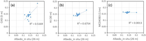
Albedo values of different resolutions cannot be compared directly over heterogeneous land surface. Figure 3 shows the relationship between in situ measurements and the satellite albedos with different spatial resolutions. As shown in the Figure 3, the determination coefficients (R²) vary with the spatial resolution of satellite albedo imagery. When the footprint of satellite data is more approximate to that of the in situ measurements, the satellite observation would be better correlated with the in situ data. Therefore, the in situ measurements should be scaled up to corresponding pixel scale prior to the validation.

Figure 3. Relation between the in situ measurements and satellite albedo imagery with different spatial resolutions.

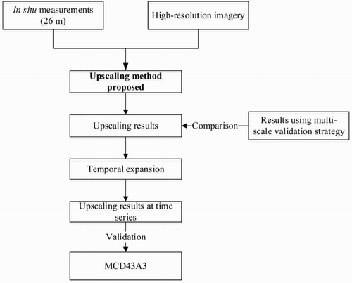
The general flowchart of the research strategy in this paper is shown in Figure 4. Firstly, the in situ albedo was upscaled with the method we proposed based on high-resolution imagery and RK technique. Then the upscaling results derived from our method were compared with the results from multi-scale validation strategy. Further, an attempt to expand this method temporally was made, and the preliminary results on time series were got. On this basis, the upscaling results with a spatial resolution of 500 m were used as the reference to validate the MODIS albedo product as a preliminary application.

Figure 4. General flowchart of the research ideas.

The method we proposed includes two key steps: trend surface establishment and residuals interpolation. The trend surface is determined by establishing a regression model between high-resolution albedo imagery and in situ albedo values. A large number of in situ observations are needed to prevent overfitting (Hengl, Heuvelink, and Rossiter 2007). For residuals interpolation, a variogram model should be first determined. Sufficient in situ observations are recommended for a stable variogram (Kang, Jin, and Li 2015).

However, a large number of in situ measurements are difficult to acquire for most cases, even in HiWATER, only 17 in situ albedos with a footprint of 26 m were available during a single period in our study area, which fails to meet the above requirements. High-resolution (higher than the footprint of original in situ measurements) imagery can provide more detailed spatial distribution information about the surface albedo within the footprint of in situ measurements and thus help to produce more in situ values. In this paper, CASI albedo imagery with a spatial resolution of 5 m was first used to discretize the in situ observations to generate more points for the regression model and variogram estimation. Then, the CASI albedo values were used as the environment covariates to establish the trend surface that were combined with the kriging techniques.

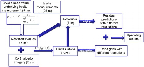
Figure 5 illustrates the upscaling flowchart using the in situ measurements and CASI albedo imagery combined with RK technique. There are six key steps during the upscaling process:

• Production of more in situ values using CASI albedo values underlying in situ measurements footprint.

• Trend surface construction based on a regression model between the newly generated in situ values and CASI albedo imagery.

• Residual calculation by removing the trend surface from surface albedo.

• The residuals interpolation to coarse scale based on kriging technique.

• The trend surface aggregation to coarse scale.

• Upscaling results calculation by adding the trend surface to the interpolated residuals at each prediction point.

Figure 5. The upscaling strategy with high-resolution imagery combined with regression-kriging.

3.1. Generation of more in situ values

The footprint of the original in situ measurements is approximately 26 m, and the spatial resolution of the high-resolution imagery used there is 5 m. Based on the method of downscaling (Wang, Xie, and Li 2014), the procedure of producing more in situ values is implemented by,(1) where N is the number of CASI pixels contained within the footprint of the ground measurements, q_i refers to CASI albedo value of ith pixel and the α is the original in situ albedo value, q_j represents the albedo value of each CASI pixel contained in the footprint of the in situ measurements, and p_i is the newly generated in situ value at the location of the ith CASI pixel. The spatial resolution of the newly generated in situ values is 5 m.

3.2. Establishment of the trend surface and calculation of residuals

We first extract the auxiliary environmental variables (CASI albedo) corresponding to the footprints of the newly generated in situ values. Then, a linear regression model (Hengl 2007) is established between the newly generated in situ values and high-resolution albedo imagery,(2) where z is the newly generated in situ albedo value, q is the auxiliary environmental variable value (CASI pixel albedo), and β are the regression coefficients, which can be estimated using the ordinary least squares (OLS) method (Hengl 2007). After the regression procedure, the trend surface of the study area and the residuals at the location of the newly generated in situ measurements can be achieved as below:(3) (4) (5) where Q is the [n, 2] matrix of CASI albedo at the n sampling locations of the newly generated in situ albedo, m(s₀) is the fitted deterministic part (trend surface), s₀ indicates the location of the point to be estimated (Hengl, Heuvelink, and Rossiter 2007) and e(s_i) is the residual at location s_i and s_i indicates the location of the newly generated in situ values.

3.3. Interpolation of residuals and aggregation of trend surface

Assuming that the residuals follow a normal distribution and satisfy the second-order stationary assumption, the variogram and the covariances of residuals were first estimated. Then the kriging weights are solved by multiplying the covariances (Hengl 2007),(6) where C is the covariance matrix derived for n × n residuals and n is the number of samples, c₀ is the vector of covariances at the new location s₀, λ₀ is the vector of the kriging weights to be derived, which is determined by the spatial dependence structure of the residual.

The residuals at the new location s₀ can be predicted,(7) where e is the vector of n residuals at primary locations. The predicted grid size is associated with the spatial scale of residuals at primary locations. Kriging variance is the weighted average of the covariances from the new point (s₀) to all calibration points, plus the Lagrange multiplier (Webster and Oliver 2001),(8) where C(s₀,s_i) is the covariance between the new location and the sampled point pair, and ϕ is the Lagrange multiplier.

The spatial resolution of the trend surface is 5 m. It can be aggregated to different resolutions (i.e. 500 m and 1 km ) using the point spread function of MODIS albedo product (Peng, Liu, Wang, et al. 2015), and this procedure does not suffer from scale effects because the regression model in Equation (2) is linear.

3.4. Prediction of upscaling results

Finally, the estimated values of surface albedo in different spatial resolutions can be obtained by adding the aggregated trend surface to the residuals kriging results at the corresponding scales,(9) where M(s₀) is the trend surface part at different spatial resolutions at location s₀, E(s₀) is the interpolated residual with different grid sizes at location s₀, and Z(s₀) is the upscaling result.

3.5. Evaluation

The accuracy of the predictions from the upscaling method are evaluated using the N-fold cross validation method (Bengio and Grandvalet 2004; Burman 1989; Kang, Jin, and Li 2015; Rodriguez, Perez, and Lozano 2010). N-fold cross validation partitions a data-set in N parts. For all observations in a part, predictions are made based on the remaining N-1 parts; this procedure is repeated for each of the N parts. The differences between the observed and predicted values are examined using RSQR (Pearson’s R²) and the root mean square deviation (RMSD). RMSD is used to measure the difference between the RK estimates and the in situ values and the RSQR is used to measure the consistency between them.

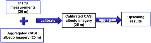
3.6. Comparison with multi-scale validation strategy

In the multi-scale validation strategy (Figure 6), the in situ measurements are used to ‘calibrate’ the CASI albedo. Because the spatial resolution of original in situ measurements (26 m) and CASI albedo imagery (5 m) is not consistent, the CASI albedo imagery was first aggregated to 25 m. Then the calibration model was determined by establishing a regression relationship between original in situ values and the 25 m CASI albedo imagery. On this basis, the 25 m CASI albedo imagery was calibrated and then aggregated to coarse spatial resolution.

Figure 6. The multi-scale validation strategy.

4. Results and discussion

4.1. Upscaling based on high resolution albedo imagery and RK technique

4.1.1. Data analysis and regression modeling of trend surface

To eliminate the effects of the order of magnitude, the newly generated in situ albedo values were transformed using scale transformation (Equation (10)) and thus the scaled albedo was derived (Becker, Chambers, and Wilks 1988). The correlations between the scaled albedo and the predictor (i.e. CASI albedo and intercept) were analyzed using the t-test statistic of the regressions (Table 2) to determine the optimal predictor and to remove the trend surface. The coefficients of the intercept for 29 June and 8 July were −5.42 and −4.5276, respectively, and the coefficient of the environmental variable (CASI albedo) were 37.1 and 25.586 for 29 June and 8 July, respectively. Both the intercept and CASI albedo coefficients were statistically significant at a more than 90% confidence level, which indicated that these two parameters were related to the surface albedo,(10) where the scaled (x) is the value after using scale transformation, mean (x) and RMSE (x) are the mean and root mean square of the variable x, respectively.

Table 2. The regression coefficients estimation and significance tests.

Predictor	29 June 2012		8 July 2012
	Intercept	CASI albedo	Intercept	CASI albedo
Estimate	−5.42	37.10	−4.53	25.59
Standard error	0.15	1.04	0.34	1.89
Pr(>|t|)	<2e−16	<2e−16	<2e−16	<2e−16
Level	***	***	***	***

Note: Significance test codes: 0 ‘***’; 0.001 ‘**’; 0.01 ‘*’; 0.05 ‘.’; and 0.1 ‘ ’ 1.

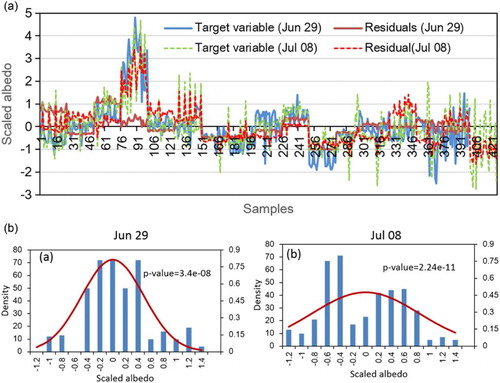
The values of the newly generated scaled in situ albedo and the residuals after removing the trend surface are shown in Figure 7(a). The in situ albedo fluctuates significantly in different locations, which indicates the heterogeneity of surface albedo over the study area. Instead, the residual values are stationary, especially for 29 June, which satisfies the assumption of kriging. In principle, the assumption of kriging is that the target variable is stationary with a normal distribution, which is probably the biggest limitation of kriging. Figure 7(b) shows a histogram of the residuals. The Shapiro–Wilk (Royston 1982) method was used to test the normality assumption, and p < .05 indicated a normal distribution (Royston 1995). It is apparent that the residual values are normally distributed significantly because the p-values shown in Figure 7(b) are much less than .05. However, the trend surface on 8 July was not removed as successfully as that on 29 June. This is because the CASI image on 8 July is not as good as on 29 June since there is a slight stripe in 8 July image. Despite this, from Figure 7(a), it can be found that the trend surface on 8 July was removed to a certain extent compared with the target variable. Fortunately, this kind of imperfection can be compensated to a certain degree by kriging the residuals. Based on the above analysis, it can be concluded that the residual variables are closer to the assumption of kriging.

Figure 7. (a) The variable value before and after the removal of the trend surface, (b) histogram of the residuals after being scaled and Shapiro–Wilk test of normality.

4.1.2. Variogram analysis for residuals kriging

After an experimental variogram has been calculated, some authorized variogram models can be used to fit it, such as linear, circular, spherical, exponential, and Gaussian models (Goovaerts 1997; Isaaks and Srivastava 1989). Figure 8 shows the point support variograms of both the in situ surface albedo measurements (a) and the residuals (b). Three universal variogram models, including Gaussian, spherical, and exponential models, were compared. The theoretical model with the smallest residual sum of squares relative to the experimental semivariograms is then selected. In this paper, the Gaussian model is the most reasonable for fitting the sample semivariograms.

Figure 8. Fitted variograms for the target variable in situ albedo (a) and residuals (b).

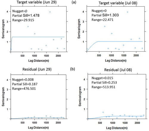
The variogram model parameters, that is, the range, sill, and nugget effect, are usually modified to fit the variogram model (Matheron 1963) to the variogram estimator. The range defines the distance from a point beyond which there is no further correlation of a biophysical property associated with that point (Cooper et al. 1997), and the spatial correlation of the samples decreases with decreases in the range values. The sill describes the maximum semivariance and is the ordinate value of the range at which the variogram levels off to an asymptote. The nugget effect depends on the variance associated with small-scale variability, measurement errors, or a combination (Noreus, Nyborg, and Hayling 1997).

As shown in Figure 8, the remaining nugget is almost the same as the original variogram; both the nugget value of the in situ albedo and the residual are approximate 0, which can be attributed to the high spatial resolution of the sampling points (5 m). There is no variance within such a small scale. The total sills of the residuals decrease compared with the target variable (in situ albedo). In this case, the sills of the residuals are dozen times smaller than that of the target variable. Furthermore, the range value of the residual is larger than that of the target variable. Smaller sill values and larger range values of the residuals indicate a more homogeneous surface. The results from the variogram analysis in Figure 8 prove that the trend is successfully removed and that the assumption of stationarity for kriging is more realistic.

4.1.3 Upscaling prediction

Once the variogram model was established, the residuals were predicted using the kriging technique and then aggregated to 30 and 500 m spatial resolutions, for evaluation and application purpose. The trend surface was also aggregated to 30 and 500 m. The final predicted results from the upscaling method we proposed are presented in Figure 9. Before analyzing the results of the spatial prediction, we need to back-transform (unscaled) the predictions to the original scale.

Figure 9. Albedo values interpolated using high-resolution imagery and regression-kriging (with a 30-m grid (left) and with a 500 m grid (right)): predictions (a) and the prediction variance (b).

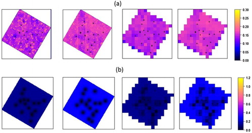
As shown in Figure 9(a), the spatial distribution of the surface albedo with a spatial resolution of 30 m is consistent with the surface features of the study area, as shown in Figure 1(c). Buildings, villages, and greenhouses present relatively high albedo values, which vary between 0.2 and 0.3, while vegetable fields, orchards, woodlands and cornfields show relatively low albedo values, which vary between 0.13 and 0.15. In particular, cornfields that have been watered (29 June) exhibit the lowest albedo values, which are approximately 0.1. The albedo values at 30 m resolution vary from 0.07 to 0.203 on 29 June and from 0.08 to 0.256 for 8 July. And the surface albedo value of 8 July is larger than that of 29 June as shown in Figure 9(a) since many cornfields have just been watered around 29 June. The result maps exhibit as much details of the spatial pattern as Figure 1(c) because CASI albedo imagery, used to establish the trend surface, can represent the heterogeneous component of surface albedo. In Figure 9(b), it can also be observed that the prediction variance is very small, which can be attributed to the fact that the residuals are more easily to satisfy the assumption of second-order stationary processes. Thus, the upscaling results, derived from the sums of the trend surface and the interpolation of the residuals, have high accuracy. Figure 9 also shows the results at a resolution of 500 m (a) and the prediction variance (b). The albedo values at 500 m vary from 0.081 to 0.169 on 29 June and from 0.102 to 0.172 on 8 July. The smaller data range are caused by the mixed land cover in the 500 m pixels, including the low albedo values of the cornfields and the high albedo values of the village. The prediction variance at a resolution of 500 m is still very small.

Further, the upscaling results with our method were evaluated using the N-fold cross validation method and compared with the initial in situ-based measurements. The RSQRs for upscaling results on 29 June and 8 July are 0.829 and 0.86, respectively. The RMSDs for the 29 June and 8 July are 0.0141 and 0.0197, respectively. The N-fold cross validation also indicates the good accuracy of the upscaling results.

4.2. Comparison with multi-scale validation strategy

To illustrate the significance of dealing with the errors that derived from calibration process (regression only), the multi-scale validation strategy was compared with to the upscaling results with the method proposed. In the multi-scale validation strategy, the CASI-based albedo were calibrated with in situ observations and then aggregated to a coarse pixel scale. Figure 10 compares the aggregated calibrated CASI albedo with the reference value (upscaling results with our method) at a spatial resolution of 500 m. It can be found there is a big difference. The upscaling results with our method show a wider dynamic range. Without the post-residual upscaling step, the aggregated CASI albedo after being calibrated shows a narrow one. Thus, regression only cannot capture fully the spatial characteristic of surface albedo. The comparison result shows that the upscaling results with our method can reflect more details about the spatial distribution characteristic of surface albedo.

Figure 10. Scatterplots between the upscaling results and averaged calibrated CASI-based albedo at a spatial resolution of 500 m. The ‘Reference_500m’ refers to the upscaling results with the method we proposed and the ‘CASI_Calibrated_500m’ is the upscaling results using multi-scale validation strategy.

In fact, the calibration process is similar to the procedure of the establishment of the trend surface as illustrated in Section 3.2, which is performed through a regression relationship between the in situ values and CASI albedo imagery. The aggregation of calibrated CASI albedo imagery can be regarded as the procedure of aggregation of trend surface. In our method, the residuals, which are positive or negative, as the random component of surface albedo, can reflect more details about surface albedo. And this component will expand the data range of upscaling results. However, in the multi-scale validation strategy, the discrepancies between the in situ values and the calibrated CASI albedo imagery, which is counterpart of the residuals in our method, are neglected. Hence, the aggregated calibrated CASI albedo is relatively concentrated. This result demonstrates the significance of a good upscaling strategy during the validation process. Based on the above discussion, it is clear that the upscaling strategy proposed in this paper can accurately capture the heterogeneity of surface albedo and provide a reliable reference for the validation of coarse resolution albedo products.

4.3. Temporal expansion

Assuming that there is no significant change in spatial distribution character of surface albedo within 5 days, the trend surface can accurately represent the heterogeneous component of surface albedo around the day when the high-resolution imagery was acquired. Although there is little fluctuations of in situ albedo during this period, such little fluctuations can be compensated to a certain degree by kriging the residuals.

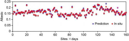
The results of upscaling were evaluated using the original in situ measurements. Because the footprint of the in situ measurements is 26 m, only the results at the 30-m resolution are chosen to represent the average condition of the upscaling predictions. Figure 11 compares the upscaling results with the original in situ measurements at the 17 WSN nodes during this period. As shown in Figure 11, the results match up quite well with the original in situ values. Both kinds of values show reasonable variation spatially and temporally. A few discrepancies between upscaling results and in situ measurements may be attributed to the effect of overfitting of the regression model. In addition, the limited ability of the trend surface to represent the spatial–temporal characteristics of surface albedo is also a contributor to the outliers.

Figure 11. Comparison between the in situ measurements and the interpolated results using high-resolution imagery combined with regression-kriging.

Scatterplots between the original in situ values and the upscaling albedo values are presented in Figure 12. Additional statistical results for the RMSE and correlation coefficient (R) values are also shown. Several outliers mentioned above are excluded for statistics. The RMSE and R for the predictions are 0.004 and 0.988, respectively. The low RMSE and high R demonstrate good accuracy of the upscaling method.

Figure 12. Scatterplots between the in situ measurements and predictions using high-resolution imagery combined with regression-kriging.

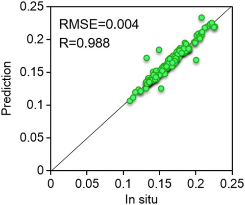
The higher albedo and lower albedo in Figure 12 represent two types of land surface over the study area. One type is high albedo value surfaces, including buildings, villages, and greenhouses. The other type is low albedo value surfaces, referring mainly to cornfields after irrigation. From this figure, we can see that the results and the original in situ values are close to 1:1. For both the high albedo value surfaces and the low albedo value surfaces, the results are almost equal to the original in situ values, which further prove the ability of the upscaling strategy to capture the surface albedo over heterogeneous land surface. Further, it can be seen that the temporal expansion of this upscaling method is practical during the short period when the spatial distribution characteristic of land surface parameters are relatively stable.

4.4. Preliminary application for assessment of MCD43A3 (V006) product

From the above analysis, the upscaling results with our method are representative of the ground value at the larger scale. The upscaling value at a spatial resolution of 500 m can be used as the most valid (unbiased) reference to directly evaluate the MCD43A3 albedo products. The MODIS product flag was also used to keep only MODIS albedo data of best quality. Scatterplots between MCD43A3 (V006) data and the upscaling results at 500 m resolution in the study area are presented in Figure 13. The RMSE and R are 0.006 and 0.61, respectively, for MCD43A3 full inversions. The small RMSE demonstrates the high accuracy of the MCD43A3 (V006) product over heterogeneous land surface. The p value of 0 and R of 0.61 demonstrates that the significant correlation between the reference and MCD43A3 albedo.

Figure 13. Scatterplots between the MCD43A3 (V006) and upscaling results at 500 spatial resolution. The dotted lines show the bias on the interval [−0.01, 0.01].

Despite the closeness of the MCD43A3 (V006) products to the upscaling results, little differences between them still exists. Nevertheless, most of the biases of MCD43A3 are within ±0.01. It should be mentioned that only full inversions were used for evaluation because the number of magnitude inversions was so few that the results were not statistically significant.

5. Conclusions

The application of land surface remote sensing albedo products in scientific research depends on their accuracy. Thus, the accuracy of different albedo products must be assessed prior to use. However, direct comparison of in situ ‘point/plot’ measurements (dozens of meters scale) with coarse-scale albedo products is not feasible over most natural landscapes because of the vast differences of spatial scales. The key issue in the albedo product validation is the upscaling process from the in situ ‘point’ measurements to coarse pixel resolutions.

In the case of land surface heterogeneity, a large number of in situ measurements should be deployed based on the optimal sampling method to capture the spatial–temporal variation of surface albedo. However, for the case of only one node within the coarse pixel, in situ observations are not enough to provide information for upscaling because of their limited footprints. Thus, high resolution remotely sensed albedo imagery should be introduced as the auxiliary information to provide the spatial distribution pattern of surface albedo.

Based on the idea of multi-scale validation strategy, this paper proposed an upscaling method based on in situ measurements and high-resolution albedo imagery combined with RK technique. To overcome the insufficient number of in situ measurements, the high-resolution imagery was first used to producing more in situ values based on a downscaling method. On this basis, the trend surface, which represents the heterogeneous component of surface albedo, and the residuals, which is the random component of surface albedo, can be derived. Cross validation shows the high accuracy of the upscaling method with RSQRs larger than 0.82 and the RMSDs smaller than 0.0197. The upscaling results are consistent with the surface features of the study area, and accurately reflect the spatial pattern of the albedo over the heterogeneous land surface. The reason is that not only the heterogeneous component of surface albedo was dealt with, but also the random component in the form of residuals.

Comparisons with the upscaling results of multi-scale validation strategy were also analyzed. The results indicated that our proposed method had wider dynamic range than that of multi-scale validation strategy and can capture more details of spatial distribution information of surface albedo. The reason can be explained by that the residuals between the in situ values and the calibrated high-resolution albedo imagery have been considered. Based on these results, we can conclude that the upscaling method, based on in situ observation and high-resolution imagery combined with RK technique, can not only overcome the scale mismatch between in situ observation and coarse-scale albedo product, but also produce more accurate results than traditional multi-scale validation strategy.

Further, this upscaling method can be expanded in the time series assuming that the spatial distribution characteristic of surface albedo is stable within a short period. The evaluation with original in situ measurements shows the upscaling method has high accuracy with an RMSE of 0.004 and R of 0.988. Because of its good performance, the upscaling results at 500 m from the in situ measurements in the HiWATER experiment were used as the reference to validate the 500 m MCD43A3 (V006) product.

Despite the reasonable results of the upscaling method, several problems still should be addressed. First, the accuracy of the upscaling results is associated with the spatial distribution of WSN nodes. It is important to remember that the ground sensors only cover the dominated land cover types, which will introduce errors to both the construction of trend surface and residual kriging. Joint observation with other land cover types which contain the heterogeneous information of surface albedo is required. Second, due to regression modeling process, there are some problems related to overfitting, reducing the prediction accuracy of the upscaling method. Last, the accuracy of the upscaling results is highly dependent on the quality of high-resolution imagery. An incorrect high-resolution imagery may lead a bad result.

The deficiency of this paper is that the high-resolution airborne imagery from CASI was acquired only on 29 June and 8 July 2012 in the HiWATER experiment. Thus, only the in situ data around these two days were used. In the future, we intend to build a universal trend surface based on the long time series in situ measurements, which will be applicable for upscaling in situ measurements in the entire time series. In conclusion, this paper provides a beneficial try for upscaling in situ measurements to coarse scales for the validation of albedo products with coarse resolutions over heterogeneous surfaces.

Acknowledgements

The authors would like to thank all of the scientists, engineers, and students who participated in the HiWATER campaigns, which provided airborne products and WSN data products for this work.

Disclosure statement

No potential conflict of interest was reported by the authors.

Additional information

Funding

This research is jointly supported by the National Basic Research Program of China under Grant 2013CB733401, the Natural Science Foundation of China under Grant nos. 41671363 and 91125003.

References

- Becker, R. A., J. M. Chambers, and A. R. Wilks. 1988. The New S Language. Pacific Grove, CA: Wadsworth & Brooks/Cole.
- Bengio, Y., and Y. Grandvalet. 2004. “No Unbiased Estimator of the Variance of K-Fold Cross-Validation.” Journal of Machine Learning Research 5 (3): 1089–1105.
- Burman, P. 1989. “A Comparative Study of Ordinary Cross-Validation, v -Fold Cross-Validation and the Repeated Learning-Testing Methods.” Biometrika 76 (3): 503–514.
- Campagnolo, M. L., Q. Sun, Y. Liu, C. Schaaf, Z. Wang, and M. O. Román. 2016. “Estimating the Effective Spatial Resolution of the Operational BRDF, Albedo, and Nadir Reflectance Products from MODIS and VIIRS.” Remote Sensing of Environment 175: 52–64.
- Cescatti, A., B. Marcolla, S. K. Santhana Vannan, J. Y. Pan, M. O. Román, X. Yang, P. Ciais, et al. 2012. “Intercomparison of MODIS Albedo Retrievals and In Situ Measurements Across the Global FLUXNET Network.” Remote Sensing of Environment 121: 323–334.
- Cheng, G. D., X. Li, W. Z. Zhao, Z. M. Xu, Q. Feng, S. C. Xiao, and H. L. Xiao. 2014. “Integrated Study of the Water-Ecosystem-Economy in the Heihe River Basin.” National Science Review 1 (3): 413–428. doi:10.1093/nsr/nwu017.
- Colgan, M. S., C. A. Baldeck, J.-B. Féret, and G. P. Asner. 2012. “Mapping Savanna Tree Species at Ecosystem Scales Using Support Vector Machine Classification and BRDF Correction on Airborne Hyperspectral and LiDAR Data.” Remote Sensing 4: 3462–3480.
- Cooper, S. D., L. Barmuta, O. Sarnelle, K. Kratz, and S. Diehl. 1997. “Quantifying Spatial Heterogeneity in Streams.” Journal of the North American Benthological Society 16: 174–188.
- Crow, W. T., A. A. Berg, M. H. Cosh, A. Loew, B. P. Mohanty, R. Panciera, P. Rosnay, D. Ryu, and J. P. Walker. 2012. “Upscaling Sparse Ground-Based Soil Moisture Observations for the Validation of Coarse-Resolution Satellite Soil Moisture Products.” Reviews of Geophysics 50 (2), doi:10.1029/2011RG000372.
- Dickinson, R. E. 1995. “Land Processes in Climate Models.” Remote Sensing of Environment 51: 27–38.
- Fan, L., Q. Xiao, J. Wen, Q. Liu, Y. Tang, D. You, H. Wang, Z. Gong, and X. Li. 2015. “Evaluation of the Airborne CASI/TASI Ts-VI Space Method for Estimating Near-Surface Soil Moisture.” Remote Sensing 7 (3): 3114–3137.
- Feingersh, T., E. Ben-Dor, and S. Filin. 2010. “Correction of Reflectance Anisotropy: A Multi-Sensor Approach.” International Journal of Remote Sensing 31: 49–74.
- Ge, Y., Y. Liang, J. Wang, Q. Zhao, and S. Liu. 2015. “Upscaling Sensible Heat Fluxes With Area-to-Area Regression Kriging.” IEEE Geoscience and Remote Sensing Letters 12 (3): 656–660.
- Goovaerts, P. 1997. Geostatistics for Natural Resources Evaluation. New York: Oxford University Press, 496 pp.
- Hengl, T. 2007. A Practical Guide to Geostatistical Mapping of Environmental Variables. Joint Research Centre, Luxemburg, IA, USA, Tech. Rep., EUR.
- Hengl, T., G. B. Heuvelink, and D. G. Rossiter. 2007. “About Regression-Kriging: From Equations to Case Studies.” Computers & Geosciences 33 (10): 1301–1315.
- Isaaks, E. H., and R. M. Srivastava. 1989. An Introduction to Applied Geostatistics. New York: Oxford University Press, 542 pp.
- Jiao, Z. T., J. D. Wang, L. O. Xie, H. Zhang, G. J. Yan, L. M. He, and X. W. Li. 2005. “Initial Validation of MODIS Albedo Product by Using Field Measurements and Airborne Multiangular Remote Sensing Observations.” Journal of Remote Sensing 9 (1): 64–72.
- Jin, R., X. Li, B. P. Yan, W. M. Luo, X. H. Li, J. W. Guo, M. G. Ma, J. Kang, Y. Zhang. 2012. “Introduction of Eco-Hydrological Wireless Sensor Network in the Heihe River Basin.” Advances in Earth Science 27: 993–1005. (in Chinese)
- Jin, Y., C. B. Schaaf, C. E. Woodcock, F. Gao, X. Li, A. H. Strahler, W. Lucht, and S. Liang. 2003. “Consistency of MODIS Surface Bidirectional Reflectance Distribution Function and Albedo Retrievals: 2. Validation.” Journal of Geophysical Research 108: 4159. doi:10.1029/2002JD002804.
- Kang, J., R. Jin, and X. Li. 2015. “Regression Kriging-Based Upscaling of Soil Moisture Measurements From a Wireless Sensor Network and Multiresource Remote Sensing Information Over Heterogeneous Cropland.” IEEE Geoscience and Remote Sensing Letters 12 (1): 92–96.
- Li, X. 2014. “Characterization, Controlling, and Reduction of Uncertainties in the Modeling and Observation of Land-Surface Systems.” Science China Earth Sciences 57 (1): 80–87.
- Li, X., G. Cheng, S. Liu, Q. Xiao, M. Ma, R. Jin, T. Che, et al. 2013. “Heihe Watershed Allied Telemetry Experimental Research (HiWATER): Scientific Objectives and Experimental Design.” Bulletin of the American Meteorological Society 94 (8): 1145–1160.
- Liang, S. 2001. “Narrowband to Broadband Conversions of Land Surface Albedo. I. Algorithms.” Remote Sensing of Environment 76: 213–238.
- Liang, S. 2003. “A Direct Algorithm for Estimating Land Surface Broadband Albedos from MODIS Imagery.” IEEE Transactions on Geoscience and Remote Sensing 41: 136–145.
- Liang, S. 2005. Quantitative Remote Sensing of Land Surfaces. New York: Wiley.
- Liang, S., H. Fang, M. Z. Chen, C. J. Shuey, C. Walthall, C. Daughtry, J. Morisette, C. Schaaf, and A. Strahler. 2002. “Validating MODIS Land Surface Reflectance and Albedo Products: Methods and Preliminary Results.” Remote Sensing of Environment 83 (1–2): 149–162. doi:10.1016/S0034-4257(02)00092-5.
- Liu, H. Y., X. G. Yang, Q. Zhang, R. Y. Wang, S. Wang, H. L. Wang, and K. Zhang. 2009. “Contrast of Ground Surface Radiation-Energy Balance in Summer and Winter on Dunhuang Gobi.” Journal of Desert Research 29 (3): 558–565.
- Lucht, W., C. B. Schaaf, and A. H. Strahler. 2000. “An Algorithm for the Retrieval of Albedo from Space Using Semiempirical BRDF Models.” IEEE Transactions on Geoscience and Remote Sensing 38: 977–998.
- Matheron, G. 1963. “Principles of Geostatistics.” Economic Geology 58 (8): 1246–1266.
- Mira, M., M. Weiss, F. Baret, D. Courault, O. Hagolle, B. Gallego-Elvira, and A. Olioso. 2015. “The MODIS (Collection v006) BRDF/Albedo Product MCD43D: Temporal Course Evaluated Over Agricultural Landscape.” Remote Sensing of Environment 170: 216–228.
- Noreus, J. P., M. R. Nyborg, and K. L. Hayling. 1997. “The Gravity Anomaly Field in the Gulf of Bothnia Spatially Characterized from Satellite Altimetry and In Situ Measurements.” Journal of Applied Geophysics 37 (2): 67–84.
- Peng, J. J., Q. Liu, L. Wang, Q. Liu, W. Fan, M. Lu, and J. G. Wen. 2015. “Characterizing the Pixel Footprint of Satellite Albedo Products Derived from MODIS Reflectance in the Heihe River Basin, China.” Remote Sensing 7 (6): 6886–6907.
- Peng, J. J., Q. Liu, J. G. Wen, Q. H. Liu, Y. Tang, L. Z. Wang, B. C. Dou, et al. 2015. “Multi-Scale Validation Strategy for Satellite Albedo Products and its Uncertainty Analysis.” Science China Earth Sciences 58: 573–588. doi:10.1007/s11430-014-4997-y.
- Pinty, B., and M. Verstraete. 1994. “On the Design and Validation of Surface Bidirectional Reflectance and Albedo Models.” Remote Sensing of Environment 41: 155–167.
- Qu, Y., Q. Liu, S. Liang, L. Wang, N. Liu, and S. Liu. 2014. “Direct-estimation Algorithm for Mapping Daily Land-Surface Broadband Albedo from MODIS Data.” IEEE Transactions on Geoscience and Remote Sensing 52: 907–919.
- Qu, Y. H., Y. Zhu, W. Han, J. Wang, and M. Ma. 2014. “Crop Leaf Area Index Observations With a Wireless Sensor Network and Its Potential for Validating Remote Sensing Products.” IEEE Journal of Selected Topics in Applied Earth Observations and Remote Sensing 7 (2): 431–444. doi:10.1109/JSTARS.2013.2289931.
- Rodriguez, J. D., A. Perez, J. A. Lozano. 2010. “Sensitivity Analysis of k-Fold Cross Validation in Prediction Error Estimation.” IEEE Transactions on Pattern Analysis and Machine Intelligence 32 (3): 569–575.
- Royston, J. P. 1982. “An Extension of Shapiro and Wilk’s W Test for Normality to Large Samples.” Applied Statistics 31: 115–124.
- Royston, P. 1995. “Remark AS R94: A Remark on Algorithm AS 181: The W-Test for Normality.” Applied Statistics 44: 547–551.
- Sailor, D. J., K. Resh, and D. Segura. 2006. “Field Measurement of Albedo for Limited Extent Test Surfaces.” Solar Energy 80 (5): 589–599.
- Salomon, J. G., C. B. Schaaf, A. H. Strahler, F. Gao, and Y. Jin. 2006. “Validation of the MODIS Bidirectional Reflectance Distribution Function and Albedo Retrievals Using Combined Observations from the Aqua and Terra Platforms.” IEEE Transactions on Geoscience and Remote Sensing 44: 1555–1565.
- Schaaf, C. B., Z. S. Wang, and A. H. Strahler. 2011. “Commentary on Wang and Zender – MODIS Snow Albedo Bias at High Solar Zenith Angles Relative to Theory and to In Situ Observations in Greenland.” Remote Sensing of Environment 115: 1296–1300.
- de Souza, R. B., M. M. Mata, C. A. E. Garcia, M. Kampel, E. N. Oliveira, and J. A. Lorenzzetti. 2006. “Multi-sensor Satellite and In Situ Measurements of a Warm Core Ocean Eddy South of the Brazil–Malvinas Confluence Region.” Remote Sensing of Environment 100: 52–66.
- Stroeve, J., J. E. Box, F. Gao, S. Liang, A. Nolin, and C. Schaaf. 2005. “Accuracy Assessment of the MODIS 16-day Albedo Product for Snow: Comparisons with Greenland In Situ Measurements.” Remote Sensing of Environment 94: 46–60.
- Susaki, J., Y. Yasuoka, K. Kajiwara, Y. Honda, and K. Hara. 2007. “Validation of MODIS Albedo Products of Paddy Fields in Japan.” IEEE Transactions on Geoscience and Remote Sensing 45 (1): 206–217.
- Valero, F. P., and R. J. Charlson. 2008. “Albedo-watching Satellite Needed to Monitor Change.” Nature 451 (7181): 887.
- Vermote, E. F., D. Tanré, J.-L. Deuze, M. Herman, and J.-J. Morcette. 1997. “Second Simulation of the Satellite Signal in the Solar Spectrum, 6s: An Overview.” IEEE Transactions on Geoscience and Remote Sensing 35: 675–686.
- Wang, Z., C. B. Schaaf, A. H. Strahler, M. J. Chopping, M. O. Román, Y. Shuai, C. E. Woodcock, D. Y. Hollinger, and D. R. Fitzjarrald. 2014. “Evaluation of MODIS Albedo Product (MCD43A) Over Grassland, Agriculture and Forest Surface Types During Dormant and Snow-Covered Periods.” Remote Sensing of Environment 140: 60–77.
- Wang, Y. T., D. H. Xie, and Y. H. Li. 2014. “Downscaling Remotely Sensed Land Surface Temperature Over Urban Areas Using Trend Surface of Spectral Index.” Journal of Remote Sensing 18 (6): 1169–1181.
- Wanner, W., A. H. Strahler, B. Hu, P. Lewis, J.-P. Muller, X. Li, C. L. B. Schaaf, M. J. Barnsley. 1997. “Global Retrieval of Bidirectional Reflectance and Albedo Over Land From EOS MODIS and MISR Data: Theory and Algorithm.” Journal of Geophysical Research: Atmospheres 102 (D14): 17143–17161.
- Webster, R., and M. A. Oliver. 2001. Geostatistics for Environmental Scientists (Statistics in Practice). New York: Wiley, 265 pp.
- Wen, J. G., Q. Liu, Q. Liu, Q. Xiao, and X. Li. 2009. “Parametrized BRDF for Atmospheric and Topographic Correction and Albedo Estimation in Jiangxi Rugged Terrain, China.” International Journal of Remote Sensing 30: 2875–2896.
- Wu, X. D., Q. Xiao, J. G. Wen, Q. Liu, J. J. Peng, and X. W. Li. 2014. “Advances in Uncertainty Analysis for the Validation of Remote Sensing Products: Take Leaf Area Index as Example.” Journal of Remote Sensing 18 (5): 1011–1023.
- Xiao, Q., and J. Wen. 2012. “HiWATER: Visible and Near-Infrared Hyperspectral Radiometer.” Accessed 29 June 2012. http://www.heihedata.org/data/1e7e8a06-1e10-4fd3-a94e-d83e463a835e, doi:10.3972/hiwater.012.2013.db; Accessed 7 July 2012. http://www.heihedata.org/data/f0b641b4-d7a8-4186-a002-7f7078d96103, doi:10.3972/hiwater.011.2013.db
- Xu, Z., S. Liu, X. Li, S. Shi, J. Wang, Z. Zhu, and M. Ma. 2013. “Intercomparison of Surface Energy Flux Measurement Systems Used During the HiWATER-MUSOEXE.” Journal of Geophysical Research: Atmospheres 118 (23): 13–140.
- You, D., J. G. Wen, Q. Xiao, Q. Liu, J. J. Peng, Q. H. Liu, Y. Tang, and B. C. Dou. 2015. “Development of a High Resolution BRDF/Albedo Product by Fusing Airborne CASI Reflectance with MODIS Daily Reflectance in the Oasis Area of the Heihe River Basin, China.” Remote Sensing 7: 6784–6807.
- Zhang, X., S. Liang, K. Wang, L. Li, and S. Gui. 2010. “Analysis of Global Land Surface Shortwave Broadband Albedo from Multiple Data Sources.” IEEE Journal of Selected Topics in Applied Earth Observations and Remote Sensing 3: 296–305.
- Zhang, R. H., J. Tian, Z. L. Li, H. B. Su, S. H. Chen, and X. Z. Tang. 2010. “Principles and Methods for the Validation of Quantitative Remote Sensing Products.” Science China Earth Sciences 53 (5): 741–751.