Quantifying water stress effect on daily light use efficiency in Mediterranean ecosystems using satellite data

ABSTRACT

The capacity of six water stress factors (ε′_i) to track daily light use efficiency (ε) of water-limited ecosystems was evaluated. These factors are computed with remote sensing operational products and a limited amount of ground data: ε′₁ uses ground precipitation and air temperature, and satellite incoming global solar radiation; ε′₂ uses ground air temperature, and satellite actual evapotranspiration and incoming global solar radiation; ε′₃ uses satellite actual and potential evapotranspiration; ε′₄ uses satellite soil moisture; ε′₅ uses satellite-derived photochemical reflectance index; and ε′₆ uses ground vapor pressure deficit. These factors were implemented in a production efficiency model based on Monteith’s approach in order to assess their performance for modeling gross primary production (GPP). Estimated GPP was compared to reference GPP from eddy covariance (EC) measurements (GPP_EC) in three sites placed in the Iberian Peninsula (two open shrublands and one savanna). ε′_i were correlated to ε, which was calculated by dividing GPP_EC by ground measured photosynthetically active radiation (PAR) and satellite-derived fraction of absorbed PAR. Best results were achieved by ε′₁, ε′₂, ε′₃ and ε′₄ explaining around 40% and 50% of ε variance in open shurblands and savanna, respectively. In terms of GPP, R² ≈ 0.70 were obtained in these cases.

KEYWORDS:

• Light use efficiency
• water stress
• GPP
• Monteith
• Mediterranean ecosystems

1. Introduction

Carbon exchange fluxes between biosphere and atmosphere play a critical role in the study of climate variability (IPCC 2007; Waring and Running 2007). Remote sensing appears as a convenient tool for monitoring these fluxes since it offers the possibility of estimating them from local to global scale and at different temporal resolutions. In this context, gross primary production (GPP), that is, the amount of carbon dioxide that vegetation uptakes from atmosphere when performing photosynthesis, can be calculated through production efficiency models (PEMs) using Monteith’s approach (Monteith 1972). This approach assumes GPP as the product of absorbed photosynthetically active radiation by vegetation (APAR) and light use efficiency (ε). Light use efficiency (also known as efficiency conversion) takes into account the efficiency of the photosynthetic process as well as the unit conversion (from energy units to mass units). PEMs usually compute APAR as the product of PAR (incoming solar radiation between 400 and 700 nm) and f_APAR (fraction of absorbed PAR), which is often estimated through a linear relationship with a vegetation spectral index (Ma et al. 2014; Wagle et al. 2014; Xiao et al. 2004b) or through the use of the index itself (Xiao et al. 2004a). PAR can be retrieved from meteorological stations or remote sensing data (Moreno et al. 2013).

ε is the most controversial input in PEMs (Garbulsky et al. 2010), and its relationship with air temperature, water availability and solar radiation conditions has been reported in the literature (Coops et al. 2010; Garbulsky et al. 2010). For operational applications, ε can be expressed as the product of an ε_max, which is a biome-specific physiological parameter describing photosynthetic activity under optimal conditions (Garbulsky et al. 2010), and a series of dimensionless factors that account for the reduction in efficiency due to different types of stress and range between 0 (total inhibition) and 1 (no inhibition). The most important stresses, depending on local eco-climatic conditions, are those due to thermal and water limitations (Garbulsky et al. 2010). It has been demonstrated that, in Mediterranean environments, water stress affects significantly ε, explaining most of its inter-annual variability (Garbulsky et al. 2008; Moreno et al. 2012), whereas air temperature contributes only marginally (Gilabert et al. 2015).

Different methods have been proposed in the last years to account for water stress within PEMs. Precipitation and potential evapotranspiration (PET) are the inputs of the soil moisture (SM) submodel in the CASA model (Potter et al. 1993, 2003) for the estimation of monthly global net ecosystem exchange. A similar approach was used by Maselli et al. (2009) in order to account for the short-term effect of summer water stress in Mediterranean forests. Vapor pressure deficit (VPD, Anderson 1936) and SM are the inputs of two of the ε reducing factors in GLO-PEM (Cao et al. 2004). Land surface water index (a normalized difference between reflectance in the near infrared and in the shortwave infrared regions) was included in the vegetation photosynthesis model (Xiao et al. 2004a, 2004b) and in the photosynthetic capacity model (Gao et al. 2014). VPD has been continuously used in MOD17 algorithm (Heinsch et al. 2006; Running and Zhao 2015) for the estimation of global gross and net primary productivity since March 2000. SM and evaporative fraction were included in C-Fix by Verstraeten, Veroustraete, and Feyen (2006) to improve the net ecosystem productivity estimation in different water-limited scenarios. Evaporative fraction was used as the downward-regulation factor accounting for water stress in EC-LUE for the estimation of daily gross primary productivity (Yuan et al. 2007).

The primary goal of the present work is to evaluate six alternatives to account for the short-term water stress when implemented in a PEM by using remote sensing imagery and the least possible amount of ancillary data, and to choose one of them for its regular use in an operative methodology for the estimation of daily GPP in Mediterranean ecosystems. The first four alternatives rely on different approaches of a water balance, the fifth one uses the photochemical reflectance index (PRI, Gamon, Peñuelas, and Field 1992), and the sixth one uses VPD.

The assessment of the six water stress factors was carried out by comparison between estimated ε (ε′_i with i = 1, 2, 3, 4, 5, and 6) and reference ε derived from eddy covariance (EC) GPP (GPP_EC) and APAR calculated multiplying in situ measured PAR by satellite-derived f_APAR. An additional analysis was performed by comparing the different GPP estimates (GPP′_i with i = 1, 2, 3, 4, 5, and 6) to GPP_EC observations. In all cases, daily values throughout several years were used depending on the length of the EC data series. The study provides indications to choose one of the six factors for the operational estimation of daily GPP in Mediterranean environments.

2. Data and sites description

2.1. Flux data

Daily Net Ecosystem Exchange data collected from three EC towers placed in the Iberian Peninsula belonging to the European Fluxes Database Cluster (http://www.europe-fluxdata.eu) were used to estimate daily GPP as explained in Reichstein et al. (2005). The main characteristics of the study sites are provided in Table 1.

Table 1. Descriptive information of the study sites.

Site	Lat (°)	Lon (°)	h (m)	T (°C)	PRE (mm)	PET (mm)	Vegetation type	Data period
ES-CPa	39.2242	−0.9031	810	13	470	1448	Open shrubland	2009–2011
ES-LJu	36.9266	−2.7521	1590	12	475	1507	Open shrubland	2005, 2008, 2011
ES-LMa	39.9415	−5.7734	260	17	600	1358	Savanna	2005–2013

Note: h is the elevation from the sea level, T is the average mean annual air temperature, PRE is the average annual precipitation, and PET is the average annual potential evapotranspiration.

The ES-CPa site is a Mediterranean shrubland located on a plateau at 810 m in the province of Valencia. Climate is typically Mediterranean subarid with warm and dry summers. Vegetation corresponds to a typical Mediterranean shrubland dominated by shrub species, such as Rosmarinus officinalis L., Ulex parviflorus Pourret, Quercus coccifera L., Juniperus oxycedrus, and Thymus sp. mixed with annual herbaceous species dominated by Brachypodium retusum. Shrub cover is about 50–60% and total vegetation cover (including herbaceous species) is about 75%.

The ES-LJu site is a Mediterranean shrubland located on a subalpine plateau at an altitude of 1590 m in the Sierra de Gádor in the province of Almería. Climate is Mediterranean subhumid. The total vegetation cover is about 50%. The actual vegetation is the result of natural regeneration after fire and it is dominated by two perennial species: Festuca scariosa and Genista pumila, with cover fractions of 19% and 12%, respectively.

The ES-LMa site is a holm oak savanna located at approximately 260 m in the province of Cáceres. Climate is Mediterranean with warm and dry summers, but with relatively cold winters due to its rather continental location. The long-term historical management at the site has resulted in a holm oak (Quercus ilex) savanna with a tree density of ca. 20–25 trees per hectare, with a mean height of 8 m. The understory vegetation is dominated by a high biodiversity of annual herbaceous species, with typical senesce by the end of May.

2.2. Meteorological data

Daily incoming global solar radiation and mean air temperature time series measured at the sites where EC towers are placed were used.

Daily maximum and minimum air temperatures and precipitation time series from in situ measurements provided by AEMet taken in 400 meteorological stations distributed around the Iberian Peninsula were interpolated by ordinary kriging to build 1-km spatial resolution images during the period 2005–2012.

Daytime daily VPD was calculated as the difference between daytime saturated vapor pressure and daily vapor pressure (Running and Zhao 2015). Hourly average air temperature and specific humidity and vapor pressure data provided by Global Modeling and Assimilation Office (GMAO) were aggregated to daily values for the calculation of daytime saturated vapor pressure and daily vapor pressure, respectively. As daily GMAO data presents a coarser spatial resolution (0.5 latitude degrees by 0.67 longitude degrees) than AEMet-derived meteorological maps (1 km), the same spatial non-linear interpolation approach of MOD17 product to match all meteorological inputs at the same projection and spatial resolution was followed.

2.3. Satellite data

Table 2 outlines the satellite products used in this study. MODIS products MCD43A1, MCD43A2 (Schaaf et al. 2002), MOD16A2 (Mu, Zhao, and Running 2013), and MODIS/Terra Ocean Reflectance Daily L2G-Lite Global 1 km SIN Grid V006 (MODOCGA, Vermote and Wolfe 2015) for the period 2005–2013 were retrieved from the online Reverb, courtesy of the NASA EOSDIS Land Processes Distributed Active Archive Center (LP DAAC), USGS/Earth Resources Observation and Science (EROS) Center, Sioux Falls, South Dakota, reverb.echo.nasa.gov. MCD43A1 is an 8-day composite which contains the BRDF parameters k₀, k₁, and k₂ at 500-m spatial resolution. MCD43A2 contains the quality flags for MCD43A1. MOD16A2 is an 8-day composite which contains actual evapotranspiration (AET), PET, actual latent heat, potential latent heat and a quality control band at 1-km spatial resolution. AET, PET, and quality control were used. MODOCGA is a daily product that contains 1-km reflectance data from Aqua MODIS bands 8–16, which are bands mostly used to produce ocean products, but the tiles contain land reflectance in this case. Bands 11, 12, and quality control were used.

Table 2. Satellite products used in the study.

	Product	Variables	Use
MODIS	MCD43A1	BRDF parameters k0, k1, and k2 (8-day composites at 500-m spatial resolution).	fAPAR calculation
	MCD43A2	MCD43A1 quality flags.	fAPAR calculation
	MOD16A2	AET and PET (8-day composites at 1-km spatial resolution).	ε′3 calculation
	MODOCGA	Daily reflectance data from AQUA bands 11 and 12 at 1-km spatial resolution and their quality flag band.	ε′5 calculation
SEVIRI	LSA-07	30-minute downward surface shortwave flux at 3-km spatial resolution (MDSSF).	PAR and ε′1 and ε′2 calculations
	LSA-09	Daily integrated LSA-07 (DIDSSF).	PAR and ε′1 and ε′2 calculations
	LSA-16	30-minute AET at 3-km spatial resolution (MET).	ε′2 calculation
	LSA-17	Daily integrated LSA-16 (DMET).	ε′2 calculation
SMOS-derived	L4SMv3D	Daily SM in the first top 5 cm at 1-km spatial resolution from the synergy between SMOS L2 SM descending orbits and MODIS-derived LST and NDVI.	ε′4 calculation
	Land cover	Hybrid land-cover map for Spain obtained from CGL2000, CORINE, IGBP, and GlobCover at 1-km spatial resolution.	Vegetation type assignation for ε′6 calculation and εmax assignation

SEVIRI products LSA-07 (down-welling surface shortwave flux estimated every 30 minutes, MDSSF) and LSA-09 (daily integrated down-welling surface shortwave flux, DIDSSF) (Product User Manual Down-welling Surface Shortwave Flux (DSSF) 2011) for the period 2007–2013, and LSA-16 (AET estimated every 30 minutes, MET) and LSA-17 (daily integrated AET, DMET) (Product User Manual Evapotranspiration (ET) 2015) for the period 2009–2013, were downloaded from the LSA SAF Server (http://landsaf.meteo.pt). These images were reprojected to a 1-km spatial resolution latitude/longitude regular grid (Moreno et al. 2013). DIDSSF and DMET were used when available or calculated by daily integration of MDSSF and MET, respectively, when not available. DIDSSF gaps were filled with global incoming solar radiation images obtained by the application of artificial neural networks to the air temperature and precipitation images mentioned above (Moreno, Gilabert, and Martínez 2011). Both products have been previously validated (Moreno, Gilabert, and Martínez 2011; Moreno et al. 2013) and a relationship between the two sources was found to apply the gap-filling procedure. DIDSSF for years 2005 and 2006 was also obtained this way.

The SMOS L4 daily regional SM product v.3 descending orbits (L4SMv3D) from the Barcelona Expert Center (BEC) were used (Piles et al. 2014). It was found after several validation exercises that, for this study, descending orbits perform systematically better than ascending ones and that a LOESS filter is a better gap-filling option for temporal gap-filling than other tested filters. Detailed information on the choice and treatment of this product can be found in Appendix A (see Supplemental data).

A hybrid land-cover map for Spain obtained by the synergistic combination of four land-cover classifications (CGL2000, CORINE, IGBP, and GlobCover) (Pérez-Hoyos, García-Haro, and San-Miguel-Ayanz 2012) was used.

3. Methodology

The description of the six water stress factors employed in this study is summarized in Table 3. ε′₁, ε′₂, and ε′₃ are based on a simple water balance calculated as the ratio between AET and PET, which represent, respectively, the real and the ideal moist conditions of vegetation. This rationale is supported by the fact that stomata closure controls both CO₂ and H₂O fluxes in plants (Monson and Baldocchi 2014). Therefore, it can be assumed that a reduction in transpiration rate is associated with a reduction in carbon uptake and, eventually, to a reduction in photosynthesis. ε′₁ uses precipitation as a proxy of AET when it is lower than PET, otherwise ε′₁ is set to 1 (Maselli et al. 2009, 2014). The use of precipitation implies the need of accumulation of both precipitation and PET over past days in order to retrieve information about water availability from past rain events. Both in ε′₁ and ε′₂, PET was calculated using the empirical relationship proposed by Jensen and Haise (1965):(1) where R_g is the incoming global solar radiation in kJ m⁻² day⁻¹ and T_a is the mean daily air temperature in °C. The difference between ε′₂ and ε′₃ resides in the source of their inputs: in ε′₃ both AET and PET are obtained from MOD16A2, whereas DMET is used as AET in ε′₂. ε′₄ relies on SM since plants need to absorb water from soil and cannot absorb it directly from rain. From the definitions of field capacity (FC, amount of water retained in the soil against gravitation forces once drainage rate has become negligible [Colman 1944; Hunt et al. 2009; Romano, Palladino, and Chirico 2011; Veihmeyer and Hendrickson 1931, 1949]) and wilting point (WP, SM content when soil particles hold water around them so tight that plants cannot extract water from it [Assouline and Or 2014; Hunt et al. 2009; Veihmeyer and Hendrickson 1949]), one can consider that plants start suffering water stress when SM falls below FC and become totally stressed when SM falls below WP. Following this reasoning, ε′₄ was conceived as the difference between SM and WP (SM−WP) normalized by the available water capacity (AWC = FC−WP, amount of water retained in the soil readily available for plants to use it (Kirkham 2005)). This way, when ε′₄ is greater than 1 (no stress), it is set to 1 and, when it is lower than 0 (totally stressed), it is set to 0. In addition, bias problems in GPP when using SM alone as a water stress factor in a PEM (Sánchez-Ruiz et al. 2014) are solved. ε′₅ is the PRI (Gamon, Peñuelas, and Field 1992). PRI uses changes in xanthophyill pigments to track ε variations. It is a narrow band index calculated as the normalized difference between reflectance in a reference band (ρ_REF) that is non sensitive to changes in xanthophyll pigments and reflectance in a band centered at 531 nm (ρ₅₃₁), which is sensitive to changes in xanthophyll pigments:(2)

Table 3. Description of the six water stress factors.

Water stress factor	Description and data source
ε′1 = PRE/PETJ−H	PRE is the precipitation in mm m^−2 day^−1. PRE images at 1-km spatial resolution were obtained by ordinary kriging to ground data from meteorological stations. PETJ−H is the potential evapotranspiration in mm m^−2 day^−1 calculated using the Jensen–Haise empirical relationship (Equation (1)).
ε′2 = AETSEVIRI/PETJ−H	AETSEVIRI is the actual evapotranspiration in mm m^−2 day^−1 obtained from SEVIRI DMET.
ε′3 = AETMODIS/PETMODIS	AETMODIS is the actual evapotranspiration in mm m^−2 day^−1 obtained from MOD16A2. PETMODIS is the potential evapotranspiration in mm m^−2 day^−1 obtained from MOD16A2.
ε′4 = (SM–WP)/(FC–WP)	SM is the soil moisture in the first top 5 cm in m^3 m^−3 day^−1. WP is the wilting point in m^3 m^−3. FC is the field capacity in m^3 m^−3. The three variables were obtained from L4SMv3.
ε′5 = PRI	PRI is the photochemical reflectance index (Equation (2)) calculated as the normalized difference between reflectance from MODOCGA bands 12 (546–556 nm) and 11 (526–536 nm).
ε′6 = n–mVPD	VPD is vapor pressure deficit in Pa calculated as in the MOD17 algorithm (see Section 2.2). Range of application: VPDmin < VPD < VPDmax, with VPDmin and VPDmax depending on the vegetation type. They are used to calculate n and m, which are empirical parameters also depending on the vegetation type. If VPD < VPDmin, ε′6 is set to 1. If VPD > VPDmax, ε′6 is set to 0.

MODOCGA bands 12 (546–556 nm) and 11 (526–536 nm) were used as the reference band and the sensitive to xanthophyll pigments band, respectively (Coops et al. 2010; Wu et al. 2010). ε′₆ was calculated using VPD exactly as the VPD_scalar used in the MOD17 algorithm (Running and Zhao 2015). It is obtained by means of a linear ramp function that varies between 0 and 1 according to threshold values depending on the vegetation type (see Table 3).

PRE and PET in ε′₁ were accumulated over the last 60 days in the cases of ES-CPa and ES-LJu and over the last 45 days in the case of ES-LMa, according to model calibrations in previous studies (Maselli et al. 2009, 2013; Potter et al. 1993; Sánchez-Ruiz et al. 2014). For the calculation of PET in ε′₁ and ε′₂, DIDSSF was used as R_g and T_a was calculated using 1-km spatial resolution maximum and minimum air temperature images, which were obtained by applying ordinary kriging to ground data taken at meteorological stations. Since MOD16A2 is an 8-day composite, AET_MODIS and PET_MODIS were obtained applying a robust local weighted scatterplot smoothing (LOWESS) with a 17-day span to original MOD16A2 AET and PET in order to attain daily values. According to the quality control band, only the good quality land pixels with clear sky conditions were used. Both 8-day composites and daily interpolated time series were validated against data from EC towers and no significant differences were found. Correlations between 8-day MOD16A2 composites and EC estimations accumulated over the same period were 0.67, 0.13, and 0.70 for ES-CPa, ES-LJu, and ES-LMa, respectively, in the case of AET. Correlations between daily EC estimates and daily values obtained by applying the LOWESS filter to MOD16A2 8-day composites were 0.73, 0.12, and 0.69, respectively. In the case of PET, correlations between MOD16A2 8-day composites and EC estimations accumulated over the same period were 0.96, 0.85, and 0.96 for ES-CPa, ES-LJu, and ES-LMa, respectively. And correlations between daily EC estimates and daily values obtained by applying the LOWESS filter to MOD16A2 8-day composites were 0.86, 0.80, and 0.91, respectively. L4SMv3D time series from 2010 to 2013 were used as SM in ε′₄, being the first time that SMOS data are used to implement a water stress factor in a PEM. WP and FC were estimated as the 5th percentile and as the 95th percentile of the long-term L4SMv3D time series, respectively (Hunt et al. 2009; Martínez-Fernández et al. 2015, 2016). In ε′₅, only the highest quality cloud free pixels according to the quality flag information were used to calculate PRI. The result was filtered using a robust LOWESS with a 9-day span in order to reduce its noise and fill the temporal gaps produced by the removing of bad quality values. The hybrid land-cover map (Pérez-Hoyos, García-Haro, and San-Miguel-Ayanz 2012) was used to assign the vegetation type to the pixels in VPD images.

The performance of the six water stress factors (denoted as ε′_i with i = 1, 2, 3, 4, 5, and 6) is evaluated both in terms of ε and in terms of GPP.

In the first case, estimated ε′ data were compared to reference ε obtained as the ratio between GPP_EC and APAR, which was, in turn, calculated as the product of PAR and f_APAR. PAR is the 46% of incoming global solar radiation (Iqbal 1983). Daily incoming global solar radiation time series measured at the EC towers were used for the calculation of PAR. f_APAR was calculated as proposed by Roujean and Breon (1995). This algorithm relies on a linear relationship between f_APAR and the renormalized difference vegetation index (RDVI), which is calculated using near infrared (ρ_NIR) and red (ρ_RED) reflectances (RDVI = (ρ_NIR− ρ_RED)/(ρ_NIR + ρ_RED)^1/2) for an optimal angular geometry in the solar principal plane from BRDF parameters in MCD43A1. Reference ε time series were filtered using a robust LOWESS with a 9-day span in order to reduce its noise and fill missing data due to the presence of temporal gaps in GPP_EC, PAR, and/or f_APAR time series.

In the second case, daily GPP_EC data were compared to daily GPP data calculated according to the Monteith approach (Monteith 1972) using the inputs formerly described as:(3) where the maximum light use efficiency ε_max was assigned to each pixel according to the hybrid land-cover map (Pérez-Hoyos, García-Haro, and San-Miguel-Ayanz 2012) and all water stress factors but ε′₆ were rescaled between 0.5 and 1 since long-term water stress is already reflected in f_APAR and they only aim to track short-term water stress (Maselli et al. 2009; Potter et al. 1993). Although ε′₆ also aims to track only short-term water stress in this study, it was not rescaled between 0.5 and 1 in order to keep the MOD17 methodology unaltered.

In summary, after calculating all the variables described in Table 3, the methodology consisted in driving a PEM with the six different water stress factors and assessing their performance by the comparison between estimated or modeled data (ε′_i and GPP′_i) and reference data (ε and GPP). A correlation analysis was carried out both between ε′_i and ε and between GPP′_i (the GPP estimated using a PEM driven by the water stress factor ε′_i) and GPP_EC. Different statistics (Table 4) such as the relative mean biased error (rMBE), the relative mean absolute error (rMAE), and the relative root mean squared error (rRMSE) between estimated and reference GPP were calculated. In order to avoid the use of dates when low temperatures can affect photosynthesis – which can happen especially in ES-CPa and ES-LJu due to their elevation and would be counter-productive for evaluating the effect of water stress – only the dates when daily mean air temperature was greater than 15°C were considered in the correlation analysis and the calculation of statistics. This threshold in daily mean air temperature was chosen taking into account the thresholds in daily minimum air temperature used in the MOD17 algorithm for the application of the TMIN_scalar in wooded grasslands and open shrublands (Running and Zhao 2015).

Table 4. Formulation of the statistics used to compare estimated (GPP′_i) and reference (GPP_EC) GPP.

Statistic	Definition
Relative mean biased error
Relative mean absolute error
Relative root mean squared error

Note: n is the number of data pairs.

4. Results

4.1. Evaluation of light use efficiency

As an example, ε′_i time series are shown in Figure 1 together with reference ε data for ES-LMa. It is observed that ε′₁ and ε′₆ saturate to 1 very often and present the highest range of variation, whereas the rest of the alternatives hardly saturate, with ε′₃ and ε′₅ presenting considerably reduced dynamic ranges. Although due to the interpolation from 8-day values ε′₃ appears very smoothed, it tracks very well the inter-annual variation of ε. ε′₂ and ε′₄ provide a good representation of the ε inter-annual variation but also rapid temporal fluctuations.

Figure 1. Temporal variation of ε (black) and ε′_i (red) in ES-LMa. From top to bottom: i = 1, 2, 3, 4, 5, and 6.

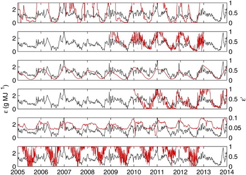
The coefficients of determination (R²) between water stress factors (ε′) and reference light use efficiency (ε) are presented in Table 5. The water stress factors based on a simple water balance achieved the best results in the three sites, explaining up to the 39% (ε′₁), the 42% (ε′₄), and the 48% (ε′₁ and ε′₂) of the reference ε variance in ES-CPa, ES-LJu, and ES-LMa, respectively. In the cases of ES-CPa and ES-LJu (open shrublands) only two (ε′₁ and ε′₃) and three (ε′₁, ε′₂, and ε′₄) water factors explained more than one-fifth of the reference ε variance, whereas in the case of ES-LMa (savanna) all the water stress factors explained at least one-fifth of this variance. No significant correlations were obtained by ε′₅ in ES-CPa and ES-LJu and by ε′₃ and ε′₆ in ES-LJu.

Table 5. Coefficients of determination (R²) between water stress factors (ε′) and reference light use efficiency (ε).

	ES-CPa	ES-LJu	ES-LMa
ε′1	0.39	0.39	0.48
ε′2	0.08	0.31	0.48
ε′3	0.24	0.01*	0.40
ε′4	0.12	0.42	0.22
ε′5	0.00*	0.02*	0.35
ε′6	0.12	0.00*	0.20

Note: Correlations were statistically significant at 95% confidence level except when marked with *. Best results appear in bold.

4.2. Evaluation of gross primary production

Figure 2 shows, for ES-LMa, (i) the daily GPP_EC time series, (ii) the daily GPP′₀ time series calculated through Equation (3) with no water stress factor, and (iii) the daily GPP_i time series calculated using Equation (3) with the six water stress factors. It can be appreciated how all alternatives reduced the GPP′₀ overestimation of GPP, especially in the spring and summer low production periods (when water stress manifests). GPP′₁ and GPP′₆ still overestimate the maximum production periods in some cases.

Figure 2. Temporal variation of GPP_EC (black), GPP′₀ (gray), and GPP′_i (red) in ES-LMa. From top to bottom: i = 1, 2, 3, 4, 5, and 6.

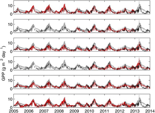
Main statistics of the comparison between estimated (GPP′_i) and reference (GPP_EC) GPP data are collected in Table 6. GPP estimates without any water stress factor (GPP′₀) were also considered. All alternatives improved coefficients of determination with respect to GPP′₀ except GPP′₅, which obtained the same R² as GPP′₀ in ES-CPa and ES-LJu, and GPP′₆ in ES-LJu that decreased R² explaining a 16% less of the GPP_EC variance than GPP′₀. In the case of ES-CPa, GPP′₁ obtained the highest coefficient of determination (R² = 0.70), although the improvement with respect to GPP′₀ was small and the six alternatives presented similar results. In the case of ES-LJu, GPP′₄ obtained the highest coefficient of determination (R² = 0.73) explaining a 30% more of the GPP_EC variance than GPP′₀. Very similar results were obtained by GPP′₂ (R² = 0.71). GPP′₁ explained a 7% more of this variance than GPP′₀, whereas GPP′₃ practically did not increase R². In the case of ES-LMa, GPP′₁ and GPP′₂ obtained the highest coefficients of determination (R² = 0.73 and R² = 0.78, respectively) explaining around a 20% more of the GPP_EC variance than GPP′₀, whereas GPP′₃, GPP′₄ and GPP′₆ only explained between a 7% and an 11% more of this variance than GPP′₀. When a water stress factor was implemented in the PEM, errors were always reduced or remained the same. The reduction of rMBE was especially strong even changing its sign in some cases.

Table 6. Statistics of the evaluation of water stress factors by comparing GPP′_i with GPP_EC. GPP₀ refers to the GPP calculated by means of Equation (3) without ε′_i.

	ES-CPa	ES-LJu	ES-LMa	ES-CPa	ES-LJu	ES-LMa
		R^2		rMBE
GPP′0	0.62	0.43	0.56	0.3	2	0.6
GPP′1	0.70	0.50	0.73	−0.14	0.7	0.08
GPP′2	0.68	0.71	0.78	−0.3	0.6	0.03
GPP′3	0.65	0.44	0.65	−0.2	0.6	−0.02
GPP′4	0.68	0.73	0.63	−0.3	0.9	−0.011
GPP′5	0.62	0.43	0.57	−0.018	1.3	0.25
GPP′6	0.69	0.27	0.67	0.05	0.3	0.04
	rMAE			rRMSE
GPP′0	0.4	2	0.7	0.5	2	0.8
GPP′1	0.3	0.8	0.3	0.4	0.9	0.4
GPP′2	0.4	0.7	0.3	0.5	0.8	0.4
GPP′3	0.4	0.8	0.3	0.5	0.9	0.4
GPP′4	0.4	0.9	0.4	0.6	1.0	0.5
GPP′5	0.3	1.3	0.5	0.4	1.4	0.5
GPP′6	0.3	0.7	0.3	0.4	0.8	0.4

Note: Correlations were statistically significant at 95% confidence level. Best results appear in bold.

It must be mentioned that different samples were used in the comparison between estimated and reference light use efficiency and GPP depending on the availability of each data source. Results were also calculated constraining the data subset to the dates when all data sources were available and they were better (R² up to 0.46, 0.59, and 0.83 for ES-CPa, ES-LJu, and ES-LMa, respectively, in the case of ε; and R² up to 0.73, 0.75, and 0.89, respectively, in the case of GPP). However, after filtering for low temperatures, only 51, 38, and 77 dates were available for ES-CPa, ES-LJu, and ES-LMa, respectively. Therefore, those results were considered as non-statistically reliable enough and all available dates in each case were used to obtain the results shown in the present study. The number of considered dates ranged from 90 when evaluating GPP′₂ in ES-LJu to 1692 when evaluating ε′₃ and ε′₅ in ES-LMa.

5. Discussion

Within PEMs based on Monteith’s approach, f_APAR is usually calculated from a vegetation index derived from the reflectances in the red and the near infrared regions of the electromagnetic spectrum (Roujean and Breon 1995), and it is therefore able to explain changes in the vegetation canopy (Gamon et al. 1995). f_APAR provides a link between the energy absorption capacity of the vegetation canopy and its structure and condition. Thus, it is able to account for changes in the vegetation canopy due to water stress. In the context of the present study, these changes would be caused by long periods of water shortage. However, these changes require some days to manifest, a delay exists between the water shortage and the structural changes that finally affect f_APAR so it cannot account for short-term water stress suffered by vegetation. Therefore, the application of Monteith’s approach to model vegetation production on a daily basis must implement a water stress factor in arid or semi-arid environments (Maselli et al. 2009).

The current experimental results indicate that the reference ε was best explained in ES-LMa (savanna) by all the water stress factors, except by ε′₄ that explained the most variance of reference ε in ES-LJu (dry open shrubland). In ES-LMa, vegetation cover is approximately distributed as 80% grassland and 20% trees (holm oaks). Grassland generally presents a very marked phenology also well explained by f_APAR (Li et al. 2010; Maselli et al. 2013; Nestola et al. 2016). When grassland dries, trees keep doing photosynthesis and water stress factors can track some of their ε decrease due to water shortage. The better performance of ε′₄ in ES-LJu than in the other two sites could be attributed to its lower vegetation fractional cover since SMOS SM estimates present higher errors over vegetated areas (Kerr et al. 2016; Lee et al. 2002), especially when vegetation is heterogeneous; and SMOS L2 successful retrievals are higher for bare soil and lower vegetation areas than for vegetated areas (http://www.cesbio.ups-tlse.fr/SMOS_blog/?page_id=1393).

As mentioned in the previous section, the water stress factors based on a water balance generally obtained the best results when trying to explain reference ε variance. Regarding to ε′₁, these results are in accordance with those found by Maselli et al. (2009) and Maselli et al. (2013) for Mediterranean forests and grasslands, respectively. This water stress factor requires the spatial interpolation of daily ground meteorological measurements, which may be problematic in rugged terrain particularly for rainfall. On the other hand, the use of ground meteorological data allows tracking rapid increases in water availability consequent on rainfall. This is only partially the case for ε′₂, which requires the spatial interpolation of ground air temperature measurements, although a downscaling of satellite AET and incoming solar global radiation must also be applied.

A temporal interpolation is needed in the cases of ε′₃ and ε′₄ to solve temporal resolution issues presented by the original products (MOD16A2 and L4SMv3D, respectively). In the case of ε′₃, an 8-day composite from daily measurements is used as input, with a consequent loss of temporal details associated with the compositing procedure. In the case of ε′₄, the applied temporal interpolation addresses the temporal undersampling (approximately one measurement each three days) of the sensor. For more details on the generation of the inputs, the reader is addressed to the references mentioned in the Section 2 of this study.

Although it has been demonstrated that PRI can track ε at plant level and local scale (Garbulsky et al. 2011; Nakaji, Oguma, and Fujinuma 2006), when calculating it through MODIS bands at regional or global scale, the signal to be detected is of the same order of magnitude of that of the sensor signal-to-noise ratio. Moreover, other factors such as geometry (view and solar angles), atmospheric correction, and the lack of the recommended reference band (centered at 570 nm) can also affect this index (Barton and North 2001; Drolet et al. 2005; Moreno et al. 2012). These issues could explain the poor performance of ε′₅ in this study.

VPD is used in MOD17 algorithm to account for changes in ε due to water stress at global scale across different ecosystem types. However, it seems not to perform as well as it would be expected in non-forest ecosystems (ES-CPa and ES-LJu) and in dry ecosystems such as savanna (ES-LMa). Other studies also found that water stress factors based on other variables than VPD such as SM improve the performance of the MOD17 production efficiency model in dry sites such as savanna (Kanniah et al. 2009) and that the ε downregulating factors should be appropriately chosen and adjusted to each study site (Turner et al. 2006).

It is notable that ε′₁ performs consistently good across the three sites, while the other five water stress factors fail in one of the sites or only achieve significant results in one of them. Although it could be expected that alternatives based on AET or SM perform better than the one based on PRE in these three Mediterranean arid sites, PRE is spatialized from ground measurements and, therefore, avoids problems that usually affect remotely sensed data.

AET in ε′₂ uses other LSA products in its algorithm such as DSSF, down-welling surface longwave flux (DSLF), and surface albedo (AL), in addition to numerical weather prediction data from the European centre for medium-range weather forecast (ECMWF), and a land-cover classification. DSSF, DSLF, and AL are affected by sensor performance, identification of clouds, atmospheric correction, surface heterogeneity, and land-cover classification. So finally the inaccuracies in the input data influence the output of the algorithm. Also the coarse spatial resolution of meteorological data (0.25° × 0.25°) from ECMWF adds uncertainties in the AET estimation, especially air temperature and specific humidity. This information can be found in ‘Algorithm Theoretical Basis Document Meteosat Second Generation Evapotranspiration (MET) Product Daily MET (DMET) Product’ (2010).

The same problems affect the estimation of AET and PET in ε′₃, which use an even coarser spatial resolution in the meteorological input data (0.5° × 0.6°) (Mu, Zhao, and Running 2013).

In the case of ε′₄, although atmospheric contribution, rain, and clouds have a negligible effect in L-band observations (Kerr et al. 2001), the original coarse spatial resolution of SMOS SM estimates and the downscaling procedure itself, which uses MODIS LST and NDVI that are affected by the problems mentioned above, could introduce some uncertainties.

ε′₅ (PRI) presents the common problems associated with the use of remotely sensed vegetation indices such as the contribution of the soil (specially in ES-CPa and ES-LJu due to their lower vegetation cover fraction), atmospheric correction, and the angular distribution of leaves and other scatterers (stems, branches, etc.), among others (Garbulsky et al. 2014). In addition, the two MODIS bands used in the study are broad enough to present interferences from other pigments reactions (Grace et al. 2007). This may partly deteriorate the performance of ε′₅ in the examined ecosystems.

In Mediterranean ecosystems, VPD varies mainly with air temperature and solar radiation, which are maximum in summer, when rainfall is almost absent. This usually yields a statistical relationship between intra-annual variation of VPD and water stress. VPD, however, can only partially account for irregular soil water recharges due to rare summer rain events, which are typical of dry Mediterranean ecosystems. In these cases, ε can increase considerably and for relatively long periods while the decreases of VPD are small and transient. This implies that also in Mediterranean areas the water stress factors based on the direct or indirect estimation of SM content should perform theoretically better than ε′₆, which was actually found in the present study and supported by previous studies (Mu et al. 2007).

Generally, the water stress factors that explained the highest amount of reference ε variance also contributed most to the improvement of the GPP estimates. Furthermore, the water stress factors that explained the less amount of reference ε variance or produced not significant correlations between reference (ε) and estimated (ε′_i) light use efficiency did not improve or even declined the performance of the PEM.

Overall, the PEM implemented in Equation (3) obtained satisfactory results independently of the used water stress factor in all the study sites. However, GPP′₂, GPP′₃, GPP′₄, and GPP′₅ present some advantages over GPP′₁ and GPP′₆: they do not need an accumulation period, and they do not require meteorological ground data except in the case of GPP′₂ that needs daily mean air temperature. This variable could be estimated from satellite land surface temperature (Nieto et al. 2011; Stisen et al. 2007; Vancutsem et al. 2010) so GPP′₂ would not require ground data either. The possibility of the estimation of daily mean air temperature from SEVIRI or MODIS land surface temperature to calculate PET and use it in GPP′₂ will be addressed in future studies. GPP′₃ and GPP′₄ presented a solid behavior among all three sites always improving the GPP estimates with respect to GPP′₀. GPP′₅ did not present any improvement in terms of R² and did not especially contribute to the reduction of uncertainties either. GPP′₆ was not the best alternative in terms of coefficient of determination between estimated and reference GPP, and it even decreased it in the case of ES-LJu, but it notably contributed to the reductions of uncertainties in the three sites.

6. Summary and conclusions

Six water stress factors calculated from operative satellite products and a limited contribution of meteorological data were proposed for their utilization as inputs in a PEM. Their performance was assessed in terms of their capacity to track intra-annual ε and GPP variability, as obtained from EC measurements taken in water-limited ecosystems. In the latter case, the water stress factors were used as drivers of a PEM (Equation (3)). Data along several years (2005–2013) from three EC tower sites located in the Iberian Peninsula were employed.

When comparing reference and estimated light use efficiency, the best results were obtained in ES-LMa (savanna), where all the water stress factors explained between 20% (ε′₆) and 48% (ε′₁ and ε′₂) of the reference ε variance. However, in ES-CPa and ES-LJu (open shrublands) not all the water stress factors achieved significant correlations and the explained reference ε variance ranged between 8% (ε′₂) and 39% (ε′₁) in ES-CPa and between 31% (ε′₂) and 42% (ε′₄) in ES-LJu.

The water stress factors were then implemented in a PEM to obtain daily GPP. The introduction of the water stress factors in the PEM generally improved its performance increasing its capability to track daily GPP intra-annual variation and reducing the difference between estimated (GPP′_i) and reference GPP data from EC measurements (GPP_EC). The most relevant improvements in terms of R² were achieved by ε′₁ (ratio between accumulated precipitation and Jensen–Haise PET), ε′₂ (ratio between SEVIRI AET and Jensen–Haise PET), ε′₃ (ratio between MOD16A2 AET and PET), and ε′₄ (SMOS-derived SM). Since the water stress factors based on a water balance using meteorological data (ε′₁ and ε′₂) obtained more reliable results, it is recommended to use them when the mentioned input data are available. However, one of the aims of the present study was to select a water stress factor able to track daily vegetation water stress for its implementation in a PEM using only remotely sensed data if possible. Therefore, ε′₃ (MOD16A2) and ε′₄ (SMOS-derived), obtaining similar results, appear as solid alternatives from an operational point of view to be included in a PEM and estimate GPP in Mediterranean ecosystems because they rely exclusively on the use of remote sensing products in their calculation and they are available at nearly real time at 1-km spatial resolution and daily temporal resolution. Until SMOS enhanced spatial resolution images are provided globally, ε′₄ could only be used for studies in the Iberian Peninsula. ε′₃, in turn, could already be applied at the global scale with the rest of the inputs of the PEM assigning a constant ε_max to all vegetation types or using a global land-cover product such as the MODIS global land-cover product MOD12.

Acknowledgements

Part of the data was kindly provided by the Spanish Meteorological Agency (AEMet), by the SMOS Barcelona Expert Center (SMOS_BEC), and by Penelope Serrano-Ortiz.

Disclosure statement

No potential conflict of interest was reported by the authors.

ORCID

Sergio Sanchez-Ruiz http://orcid.org/0000-0002-4849-9918

Alvaro Moreno http://orcid.org/0000-0003-2990-7768

Maria Piles http://orcid.org/0000-0002-1169-3098

Fabio Maselli http://orcid.org/0000-0001-6475-4600

Arnaud Carrara http://orcid.org/0000-0002-9095-8807

Steven Running http://orcid.org/0000-0001-6906-3841

Maria Amparo Gilabert http://orcid.org/0000-0002-3548-1524

Additional information

Funding

This work was partially funded by the RESET CLIMATE (CGL2012-35831), the ESCENARIOS (CGL2016-75239-R), and the PROMISES (ESP2015-67549-C3) projects from the Spanish Ministry of Economy and Competitiveness, and by the LSA SAF CDOP-2 project from the European Organization for the Exploitaition of Meteorological Satellites (EUMETSAT).

References

- Algorithm Theoretical Basis Document Meteosat Second Generation Evapotranspiration (MET) Product Daily MET (DMET) Product. 2010. “The EUMETSAT Satellite Application Facility on Land Surface Analysis (LSA SAF)”.
- Anderson, Donald B. 1936. “Relative Humidity or Vapor Pressure Deficit.” Ecology 17 (2): 277–282. doi:10.2307/1931468.
- Assouline, S., and D. Or. 2014. “The Concept of Field Capacity Revisited: Defining Intrinsic Static and Dynamic Criteria for Soil Internal Drainage.” Water Resources Research 50 (6): 4787–4802.
- Barton, C. V. M., and P. R. J. North. 2001. “Remote Sensing of Canopy Light Use Efficiency Using the Photochemical Reflectance Index Model and Sensitivity Analysis.” Remote Sensing of Environment 78: 264–273. http://hdl.handle.net/10512/999992087.
- Cao, Mingkui, Stephen D. Prince, Jennifer Small, and Scott J. Goetz. 2004. “Remotely Sensed Interannual Variations and Trends in Terrestrial Net Primary Productivity 1981-2000.” Ecosystems 7: 233–242. doi:10.1007/s10021-003-0189-x.
- Colman, E. A. 1944. “The Dependence of Field Capacity upon the Depth of Wetting of Field Soils.” Soil Science 58 (1): 43–50.
- Coops, Nicholas C., Thomas Hilker, Forrest G. Hall, Caroline J. Nichol, and Guillaume G. Drolet. 2010. “Estimation of Light-use Efficiency of Terrestrial Ecosystems from Space: A Status Report.” BioScience 60 (10): 788–797. doi:10.1525/bio.2010.60.10.5.
- Drolet, Guillaume G., Karl F. Huemmrich, Forrest G. Hall, Elizabeth M. Middleton, T. Andrew Black, Alan G. Barr, and Hank A. Margolis. 2005. “A MODIS-Derived Photochemical Reflectance Index to Detect Inter-annual Variations in the Photosynthetic Light-use Efficiency of a Boreal Deciduous Forest.” Remote Sensing of Environment 98 (2–3): 212–224. doi:10.1016/j.rse.2005.07.006.
- Gamon, John A., Christopher B. Field, Michael L. Goulden, Kevin L. Griffin, Anne E. Hartley, Geeske Joel, Josep Peñuelas, and Riccardo Valentini. 1995. “Relationships between NDVI, Canopy Structure, and Photosynthesis in Three Californian Vegetation Types.” Ecological Applications 5 (1): 28–41.
- Gamon, J. A., J. Peñuelas, and C. B. Field. 1992. “A Narrow-Waveband Spectral Index That Tracks Diurnal Changes in Photosynthetic Efficiency.” Remote Sensing of Environment. doi:10.1016/0034-4257(92)90059-S.
- Gao, Yanni, Guirui Yu, Huimin Yan, Xianjin Zhu, Shenggong Li, Qiufeng Wang, Junhui Zhang, et al. 2014. “A MODIS-Based Photosynthetic Capacity Model to Estimate Gross Primary Production in Northern China and the Tibetan Plateau.” Remote Sensing of Environment 148: 108–118. doi:10.1016/j.rse.2014.03.006.
- Garbulsky, M. F., I. Filella, A. Verger, and J. Peñuelas. 2014. “Photosynthetic Light Use Efficiency from Satellite Sensors: From Global to Mediterranean Vegetation.” Environmental and Experimental Botany 103: 3–11. doi:10.1016/j.envexpbot.2013.10.009.
- Garbulsky, Martín F., Josep Peñuelas, John Gamon, Yoshio Inoue, and Iolanda Filella. 2011. “The Photochemical Reflectance Index (PRI) and the Remote Sensing of Leaf, Canopy and Ecosystem Radiation Use Efficiencies: A Review and Meta-analysis.” Remote Sensing of Environment 115 (2): 281–297. doi:10.1016/j.rse.2010.08.023.
- Garbulsky, Martín F., Josep Peñuelas, Dario Papale, Jonas Ardö, Michael L. Goulden, Gerard Kiely, Andrew D. Richardson, Eyal Rotenberg, Elmar M. Veenendaal, and Iolanda Filella. 2010. “Patterns and Controls of the Variability of Radiation Use Efficiency and Primary Productivity across Terrestrial Ecosystems.” Global Ecology and Biogeography 19 (2): 253–267. doi:10.1111/j.1466-8238.2009.00504.x.
- Garbulsky, Martín F., Josep Peñuelas, Dario Papale, and Iolanda Filella. 2008. “Remote Estimation of Carbon Dioxide Uptake by a Mediterranean Forest.” Global Change Biology 14 (12): 2860–2867.
- Gilabert, M. A., A. Moreno, F. Maselli, B. Martínez, M. Chiesi, S. Sánchez-Ruiz, F. J. García-Haro, et al. 2015. “Daily GPP Estimates in Mediterranean Ecosystems by Combining Remote Sensing and Meteorological Data.” ISPRS Journal of Photogrammetry and Remote Sensing. International Society for Photogrammetry and Remote Sensing, Inc. (ISPRS) 102: 184–197. doi:10.1016/j.isprsjprs.2015.01.017.
- Grace, J., C. Nichol, M. Disney, P. Lewis, T. Quaife, and P. Bowyer. 2007. “Can We Measure Terrestrial Photosynthesis from Space Directly, Using Spectral Reflectance and Fluorescence?” Global Change Biology 13: 1484–1497. doi:10.1111/j.1365-2486.2007.01352.x.
- Heinsch, Faith Ann, Maosheng Zhao, Steven W. Running, John S. Kimball, Ramakrishna R. Nemani, Kenneth J. Davis, Paul V. Bolstad, et al. 2006. “Evaluation of Remote Sensing Based Terrestrial Productivity from MODIS Using Regional Tower Eddy Flux Network Observations.” IEEE Transactions on Geoscience and Remote Sensing 44 (7): 1908–1923. doi:10.1109/TGRS.2005.853936.
- Hunt, E. D., K. G. Hubbard, D. A. Wilhite, T. J. Arkebauer, and A. L. Dutcher. 2009. “The Development and Evaluation of a Soil Moisture Index.” International Journal of Climatology 29: 747–759.
- IPCC. 2007. “Coupling Between Changes in the Climate System and Biogeochemistry.” In Climate Change 2007: The Physical Science Basis. Contribution of Working Group I to the Fourth Assessment Report of the Intergovernmental Panel on Climate Change, edited by S. Solomon, D. Qin, M. Manning, Z. Chen, M. Marquis, K. B. Averyt, M. Tignor, and H. L. Miller, 499–588. Cambridge: Cambridge University Press.
- Iqbal, M. 1983. An Introduction to Solar Radiation. Toronto: Academic Press.
- Jensen, M. E., and H. R. Haise. 1965. “Estimating Evapotranspiration from Solar Radiation.” Journal of Irrigation and Drainage Division 89: 15–41.
- Kanniah, K. D., J. Beringer, L. B. Hutley, N. J. Tapper, and X. Zhu. 2009. “Evaluation of Collections 4 and 5 of the MODIS Gross Primary Productivity Product and Algorithm Improvement at a Tropical Savanna Site in Northern Australia.” Remote Sensing of Environment 113 (9): 1808–1822. doi:10.1016/j.rse.2009.04.013.
- Kerr, Y. H., A. Al-yaari, N. Rodriguez-fernandez, M. Parrens, B. Molero, D. Leroux, S. Bircher, et al. 2016. “Overview of SMOS Performance in Terms of Global Soil Moisture Monitoring after Six Years in Operation.” Remote Sensing of Environment 180: 40–63. doi:10.1016/j.rse.2016.02.042.
- Kerr, Yann H., Philippe Waldteufel, Jean-pierre Wigneron, Jean-michel Martinuzzi, Jordi Font, and Michael Berger. 2001. “Soil Moisture Retrieval from Space: The Soil Moisture and Ocean Salinity (SMOS) Mission.” IEEE Transactions on Geoscience and Remote Sensing 39 (8): 1729–1735.
- Kirkham, M. B. 2005. Principles of Soil and Plant Water Relations. Burlington, MA: Elseveir Academic Press.
- Lee, Khil-ha, Eleanor J. Burke, W. James Shuttleworth, and R. Chawn Harlow. 2002. “Influence of Vegetation on SMOS Mission Retrievals.” Hydrology and Earth System Sciences 6 (2): 153–166.
- Li, Gang, Daolong Wang, Shimin Liu, Wenjie Fan, Hua Zhang, Xiaoping Xin, and Hongbin Zhang. 2010. “Validation of Modis Fapar Products in Hulunber Grassland of China.” 2010 IEEE International Geoscience and Remote Sensing Symposium, 1047–1050, Honolulu.
- Ma, Xuanlong, Alfredo Huete, Qiang Yu, Natalia Restrepo-Coupe, Jason Beringer, Lindsay B. Hutley, Kasturi Devi Kanniah, James Cleverly, and Derek Eamus. 2014. “Parameterization of an Ecosystem Light-Use-Efficiency Model for Predicting Savanna GPP Using MODIS EVI.” Remote Sensing of Environment 154 (1): 253–271. doi:10.1016/j.rse.2014.08.025.
- Martínez-Fernández, J., A. González-Zamora, N. Sánchez, and A. Gumuzzio. 2015. “A Soil Water Based Index as a Suitable Agricultural Drought Indicator.” Journal of Hydrology 522: 265–273. doi:10.1016/j.jhydrol.2014.12.051.
- Martínez-Fernández, J., A. González-Zamora, N. Sánchez, A. Gumuzzio, and C. M. Herrero-Jiménez. 2016. “Satellite Soil Moisture for Agricultural Drought Monitoring: Assessment of the SMOS Derived Soil Water Deficit Index.” Remote Sensing of Environment 177: 277–286. doi:10.1016/j.rse.2016.02.064.
- Maselli, F., G. Argenti, M. Chiesi, L. Angeli, and D. Papale. 2013. “Simulation of Grassland Productivity by the Combination of Ground and Satellite Data.” Agriculture, Ecosystems and Environment 165: 163–172. doi:10.1016/j.agee.2012.11.006.
- Maselli, Fabio, Paolo Cherubini, Marta Chiesi, María Amparo Gilabert, Fabio Lombardi, Alvaro Moreno, Maurizio Teobaldelli, and Roberto Tognetti. 2014. “Start of the Dry Season as a Main Determinant of Inter-Annual Mediterranean Forest Production Variations.” Agricultural and Forest Meteorology 194: 197–206. doi:10.1016/j.agrformet.2014.04.006.
- Maselli, Fabio, Dario Papale, Nicola Puletti, Gherardo Chirici, and Piermaria Corona. 2009. “Combining Remote Sensing and Ancillary Data to Monitor the Gross Productivity of Water-Limited Forest Ecosystems.” Remote Sensing of Environment 113 (3): 657–667. doi:10.1016/j.rse.2008.11.008.
- Monson, Russell, and Dennis Baldocchi. 2014. Terrestrial Biosphere-Atmosphere Fluxes. New York: Cambridge University Press.
- Monteith, J. L. 1972. “Solar Radiation and Productivity in Tropical Ecosystems.” The Journal of Applied Ecology 9 (3): 747–766.
- Moreno, A., M. A. Gilabert, F. Camacho, and B. Martínez. 2013. “Validation of Daily Global Solar Irradiation Images from MSG over Spain.” Renewable Energy 60: 332–42. doi:10.1016/j.renene.2013.05.019.
- Moreno, A., M. A. Gilabert, and B. Martínez. 2011. “Mapping Daily Global Solar Irradiation over Spain: A Comparative Study of Selected Approaches.” Solar Energy 85 (9): 2072–2084. doi:10.1016/j.solener.2011.05.017.
- Moreno, A., F. Maselli, M. A. Gilabert, M. Chiesi, B. Martínez, and G. Seufert. 2012. “Assessment of MODIS Imagery to Track Light-Use Efficiency in a Water-Limited Mediterranean Pine Forest.” Remote Sensing of Environment 123: 359–367. doi:10.1016/j.rse.2012.04.003.
- Mu, Qiaozhen, Maosheng Zhao, Faith Ann Heinsch, Mingliang Liu, Hanqin Tian, and Steven W. Running. 2007. “Evaluating Water Stress Controls on Primary Production in Biogeochemical and Remote Sensing Based Models.” Journal of Geophysical Research 112. doi:10.1029/2006JG000179.
- Mu, Qiaozhen, Maosheng Zhao, and Steven W. Running. 2013. MODIS Global Terrestrial Evapotranspiration (ET) Product (NASA MOD16A2/A3) Algorithm Theoretical Basis Document Collection 5. Missoula: University of Montana.
- Nakaji, T., H. Oguma, and Y. Fujinuma. 2006. “Seasonal Changes in the Relationship between Photochemical Reflectance Index and Photosynthetic Light Use Efficiency of Japanese Larch Needles.” International Journal of Remote Sensing 27 (3): 493–509. doi:10.1080/01431160500329528.
- Nestola, Enrica, Carlo Calfapietra, Craig A. Emmerton, Christopher Y S. Wong, Donnette R. Thayer, and John A. Gamon. 2016. “Monitoring Grassland Seasonal Carbon Dynamics, by Integrating MODIS NDVI, Proximal Optical Sampling, and Eddy Covariance Measurements.” Remote Sensing 8 (3): 260–284. doi:10.3390/rs8030260.
- Nieto, Héctor, Inge Sandholt, Inmaculada Aguado, Emilio Chuvieco, and Simon Stisen. 2011. “Air Temperature Estimation with MSG-SEVIRI Data: Calibration and Validation of the TVX Algorithm for the Iberian Peninsula.” Remote Sensing of Environment 115 (1): 107–116. doi:10.1016/j.rse.2010.08.010.
- Pérez-Hoyos, A., F. J. García-Haro, and J. San-Miguel-Ayanz. 2012. “A Methodology to Generate a Synergetic Land-Cover Map by Fusion of Different: Land-Cover Products.” International Journal of Applied Earth Observation and Geoinformation 19 (1): 72–87. doi:10.1016/j.jag.2012.04.011.
- Piles, María, Nilda Sánchez, Mercè Vall-llossera, Adriano Camps, José Martínez-Fernández, Justino Martínez, and Verónica González-Gambau. 2014. “A Downscaling Approach for SMOS Land Observations: Evaluation of High-Resolution Soil Moisture Maps Over the Iberian Peninsula.” IEEE Journal of Selected Topics in Applied Earth Observation and Remote Sensing. doi:10.1109/JSTARS.2014.2325398.
- Potter, Christopher S., Steven Klooster, Ranga Myneni, Vanessa Genovese, Pang Ning Tan, and Vipin Kumar. 2003. “Continental-Scale Comparisons of Terrestrial Carbon Sinks Estimated from Satellite Data and Ecosystem Modeling 1982-1998.” Global and Planetary Change 39: 201–213. doi:10.1016/j.gloplacha.2003.07.001.
- Potter, Christopher S., James T. Randerson, Christopher B. Field, Pamela A. Matson, Peter M. Vitousek, Harold A. Mooney, and Steven A. Klooster. 1993. “Terrestrial Ecosystem Production: A Process Model Based on Global Satellite and Surface Data.” Global Biogeochemical Cycles 7 (4): 811–841.
- “Product User Manual Down-Welling Surface Shortwave Flux (DSSF).” 2011. “The EUMETSAT Satellite Application Facility on Land Surface Analysis (LSA SAF)”.
- “Product User Manual Evapotranspiration (ET).” 2015. “The EUMETSAT Satellite Application Facility on Land Surface Analysis (LSA SAF)”.
- Reichstein, Markus, Eva Falge, Dennis Baldocchi, Dario Papale, Marc Aubinet, Paul Berbigier, Christian Bernhofer, et al. 2005. “On the Separation of Net Ecosystem Exchange into Assimilation and Ecosystem Respiration: Review and Improved Algorithm.” Global Change Biology 11 (9): 1424–1439. doi:10.1111/j.1365-2486.2005.001002.x.
- Romano, N., M. Palladino, and G. B. Chirico. 2011. “Parameterization of a Bucket Model for Soil-Vegetation-Atmosphere Modeling under Seasonal Climatic Regimes.” Hydrology and Earth System Sciences 15 (12): 3877–3893. doi:10.5194/hess-15-3877-2011.
- Roujean, Jean-louis, and Francois-marie Breon. 1995. “Estimating PAR Absorbed by Vegetation from Bidirectional Reflectance Measurements.” Remote Sensing of Environment 51: 375–384.
- Running, Steven W., and Maosheng Zhao. 2015. User’s Guide: Daily GPP and Annual NPP (MOD17A2/A3) Products NASA Earth Observing System MODIS Land Algorithm. Version 3.0. Missoula: University of Montana.
- Sánchez-Ruiz, S., A. Moreno, B. Martínez, M. Piles, F. Maselli, A. Carrara, and M. A. Gilabert. 2014. “Impact of Water Stress on GPP Estimation from Remote Sensing Data in Mediterranean Ecosystems.” Proceedings 4th International Symposium on Recent Advances in Quantitative Remote Sensing, Torrent (Spain), September 22–26.
- Schaaf, Crystal B., Feng Gao, Alan H. Strahler, Wolfgang Lucht, Xiaowen Li, Trevor Tsang, Nicholas C. Strugnell, et al. 2002. “Global Albedo, BRDF and Nadir BRDF-Adjusted Reflectance Products from MODIS.” Remote Sensing of Environment 83: 135–148.
- Stisen, Simon, Inge Sandholt, Anette Norgaard, Rasmus Fensholt, and Lars Eklundh. 2007. “Estimation of Diurnal Air Temperature Using MSG SEVIRI Data in West Africa.” Remote Sensing of Environment 110 (2): 262–274. doi:10.1016/j.rse.2007.02.025.
- Turner, David P., William D. Ritts, Warren B. Cohen, Stith T. Gower, Steve W. Running, Maosheng Zhao, Marcos H. Costa, et al. 2006. “Evaluation of MODIS NPP and GPP Products across Multiple Biomes.” Remote Sensing of Environment 102 (3–4): 282–292. doi:10.1016/j.rse.2006.02.017.
- Vancutsem, Christelle, Pietro Ceccato, Tufa Dinku, and Stephen J. Connor. 2010. “Evaluation of MODIS Land Surface Temperature Data to Estimate Air Temperature in Different Ecosystems over Africa.” Remote Sensing of Environment 114 (2): 449–465. doi:10.1016/j.rse.2009.10.002.
- Veihmeyer, F. J., and A. H. Hendrickson. 1931. “The Moisture Equivalent as a Measure of the Field Capacity of Soils.” Soil Science 32: 181–194. doi:10.1097/00010694-193109000-00003.
- Veihmeyer, F. J., and A. H. Hendrickson. 1949. “Methods of Measuring Field Capacity and Permanent Wilting Percentage of Soils.” Soil Science 68 (1): 75–94.
- Vermote, E., and R. Wolfe. 2015. “MODOCGA MODIS/Terra Ocean Reflectance Daily L2G-Lite Global 1 km SIN Grid V006.” NASA EOSDIS Land Processes DAAC. doi:10.5067/MODIS/MODOCGA.006.
- Verstraeten, Willem W., Frank Veroustraete, and Jan Feyen. 2006. “On Temperature and Water Limitation of Net Ecosystem Productivity: Implementation in the C-Fix Model.” Ecological Modelling 199 (1): 4–22. doi:10.1016/j.ecolmodel.2006.06.008.
- Wagle, Pradeep, Xiangming Xiao, Margaret S. Torn, David R. Cook, Roser Matamala, Marc L. Fischer, Cui Jin, Jinwei Dong, and Chandrashekhar Biradar. 2014. “Sensitivity of Vegetation Indices and Gross Primary Production of Tallgrass Prairie to Severe Drought.” Remote Sensing of Environment 152: 1–14. doi:10.1016/j.rse.2014.05.010.
- Waring, H. R., and S. W. Running. 2007. Forest Ecosystems. 3rd ed. San Diego, CA: Academic Press.
- Wu, Chaoyang, Zheng Niu, Quan Tang, and Wenjiang Huang. 2010. “Revised Photochemical Reflectance Index (PRI) for Predicting Light Use Efficiency of Wheat in a Growth Cycle: Validation and Comparison.” International Journal of Remote Sensing 31 (11): 2911–2924.
- Xiao, Xiangming, David Hollinger, John Aber, Mike Goltz, Eric A. Davidson, Qingyuan Zhang, and Berrien Moore. 2004a. “Satellite-Based Modeling of Gross Primary Production in an Evergreen Needleleaf Forest.” Remote Sensing of Environment 89 (4): 519–534. doi:10.1016/j.rse.2003.11.008.
- Xiao, Xiangming, Qingyuan Zhang, Bobby Braswell, Shawn Urbanski, Stephen Boles, Steven Wofsy, Berrien Moore III, and Dennis Ojima. 2004b. “Modeling Gross Primary Production of Temperate Deciduous Broadleaf Forest Using Satellite Images and Climate Data.” Remote Sensing of Environment 91 (2): 256–270. doi:10.1016/j.rse.2004.03.010.
- Yuan, Wenping, Shuguang Liu, Guangsheng Zhou, Guoyi Zhou, Larry L. Tieszen, Dennis Baldocchi, Christian Bernhofer, et al. 2007. “Deriving a Light Use Efficiency Model from Eddy Covariance Flux Data for Predicting Daily Gross Primary Production across Biomes.” Agricultural and Forest Meteorology 143: 189–207. doi:10.1016/j.agrformet.2006.12.001.