Parallelizing maximum likelihood classification on computer cluster and graphics processing unit for supervised image classification

ABSTRACT

Supervised image classification has been widely utilized in a variety of remote sensing applications. When large volume of satellite imagery data and aerial photos are increasingly available, high-performance image processing solutions are required to handle large scale of data. This paper introduces how maximum likelihood classification approach is parallelized for implementation on a computer cluster and a graphics processing unit to achieve high performance when processing big imagery data. The solution is scalable and satisfies the need of change detection, object identification, and exploratory analysis on large-scale high-resolution imagery data in remote sensing applications.

KEYWORDS:

• Maximum likelihood classification
• supervised classification
• parallel computing
• graphics processing unit

1. Introduction

Image classification is a fundamental task in remote sensing applications. By differentiating and grouping pixels into different clusters, image classification helps to distinguish land cover features by different land use types, such as water bodies, forest, grass lands, urbanized and construction area, and other land use land cover types. By analyzing time series of classified imagery data, change detection and other spatial analysis can be conducted. While it was concluded that ‘No pattern classification method is inherently superior to any other’ (Jensen 2016, 362), in comparison to unsupervised classification approaches that are automated by computer programs, supervised classification provides an alternative solution by integrating human knowledge into the classification process. In this research, maximum likelihood classification (MLC) is selected from other classic approaches for supervised classification, for example, parallelepiped, minimum distance, and k-nearest neighbors, since MLC has better quality and has been adopted in commonly used software products for remote sensing and geographic information system applications. Such matured software products can be used for quality control and performance comparison in this study.

MLC is theoretically well established and has been extensively and successfully used for land cover and land use classification (Shackelford and Davis 2003; Du et al. 2012; Erener 2013). Given that high spatial resolution images are increasingly available, a huge amount of image data will need to be processed and analyzed. For this reason, accelerating MLC calculation has broader impact in real-world practice. Although MLC was regarded as parallelizable (Christophe, Michel, and Inglada 2011), the formal implementation of parallelized solutions has seldom been published. Within this research, we explored two approaches to parallelize MLC on a computer cluster by the message passing interface (MPI) approach and on a single graphics processing unit (GPU) to achieve high performance with speedup of about 30× when 400 processors were applied and about 100× when an NVIDIA K40 GPU was utilized.

In the remaining part of this paper, we first review supervised image classification and current status of parallelized supervised classification to establish the research context. Details about the MLC algorithm and its parallel implementations on central processing unit (CPU) cluster and GPU are introduced. Future directions are discussed in the conclusion.

2. Research context

Satellite imagery and aerial photos have been extensively used in analyzing land use and land cover change through different approaches for image classification. Supervised image classification algorithms include maximum likelihood, logistic regression, parallelepiped, minimum distance, and other parametric and nonparametric techniques. Unsupervised classification includes the iterative self-organizing cluster analysis (ISODATA), agglomerative hierarchical clustering, and histogram peak selection (Richards and Richards 1999). The object-based classification firstly groups pixels into homogeneous segments then classifies the segments that contain spectral and spatial features unavailable at the pixel level (Blaschke 2010). Furthermore, data mining and machine learning approaches can be used for image classification by treating pixels or pixel groups as data points (Shackelford and Davis 2003; Du et al. 2012; Li et al. 2012; Erener 2013; Lu et al. 2014).

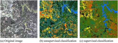
Figure 1 displays different results of image classification by unsupervised (ISODADA) and supervised (MLC) classification. In comparison to the original three band image in (a), different colors are used to differentiate five land cover categories in (b) and (c). In this case, blue color denotes water body, orange color denotes urbanized area and varied types of construction, green color denotes forest, yellow color denotes grass land, and black color denotes barren land. In general, the result of supervised classification displayed in Figure 1(c) is much more meaningful than the result derived from unsupervised classification displayed in Figure 1(b). For example, in Figure 1(b), the same type of object, such as water body, is assigned to multiple classes. In fact, the supervised classification result in Figure 1(c) was generated by merging 12 subclasses to 5 classes. Five subclasses were used to capture different spectral features of water body, while four subclasses were used to capture representative spectral information of constructed areas. As a result, the impact of intra-class variability was reduced resulting in higher accuracies in the supervised classification result.

Figure 1. Image classification by unsupervised (ISODADA) and supervised (MLC) approaches. (a) Original image, (b) unsupervised classification, (c) supervised classification.

Compared with other traditional supervised classification approaches, MLC usually has higher accuracy when the training data have high quality and are representative (Lu et al. 2014). MLC outperforms minimum distance and parallelepiped classification algorithm because MLC specifically considers the posteriori probability of training pixels, and allows for non-symmetric class distribution in the spectral domain (Richards and Richards 1999). In comparison to sophisticated machine learning algorithms, such as support vector machine and tree-based classifiers, MLC is comparable and satisfactory when pixel value distribution really conforms to Gaussian distribution as assumed by MLC (La Rosa and Wiesmann 2013; Li et al. 2014; Lu et al. 2014), while MLC does not require parameter tuning which is essential to machine learning algorithms. For this reason, MLC is selected in this research to examine how the scalability and performance of supervised classification can be enhanced and improved by utilizing clusters of computers or GPU when large volume of imagery data are processed.

Dealing with high-resolution imagery data is time consuming. When handling huge amount of pixels, even algorithms with linear time complexity require large memory space and long time for computation. For this reason, parallel and distributed computing solutions were developed to handle large-scale imagery data and to improve the computation performance, while accelerator technologies have been adopted for image processing tasks in recent years. Buchnev, Kim, and Pyatkin (2003) reviewed the distributed computing architecture and the feasibility of parallel processing of remote sensing images on an eight processor machine. Valencia et al. (2007) explored parallel processing of high-dimensional remote sensing images using cluster computer architectures. Christophe, Michel, and Inglada (2011) discussed remote sensing processing by multicore and GPU. Plaza (2006) discussed the trend and perspective of heterogeneous parallel computing in remote sensing applications, and consequently published hundreds of papers in this research front.

In the case of image classification, Wu et al. (2015) discussed a sparse representation and Markov random fields based spatial-spectral classifier for hyperspectral image classification over a heterogeneous CPU–GPU system. Chang et al. (2011) discussed a parallel implementation of the positive Boolean function for remote sensing image classification on multi-computer and multiprocessor systems. Bernabé et al. (2012) discussed GPU implementations for image morphological operations, k-means, and image convolution to support the need of real-time processing of Google-Map satellite images. Shi et al. (2014) parallelized the ISODATA algorithm for unsupervised classification on three supercomputers with heterogeneous architectures, that is, a CPU cluster, a GPU cluster, and an Intel's Many-Integrated Core cluster, respectively.

Currently very limited work has been done on the parallelization of MLC. When Christophe, Michel, and Inglada (2011) discussed remote sensing processing by multicore and GPU, MLC was mentioned but not implemented. Instead, the Normalized Difference Vegetation Index was the use case applied in their research. Bernabé et al. (2012) also mentioned MLC in their proposed processing chain but the authors used software ENVI (i.e. ENvironment for Visualizing Images) to complete MLC. What was parallelized on GPU is ‘the processing chain (including morphological pre-processing, k-means clustering, and spatial post-processing)’ (Bernabé et al. 2012) but MLC was not included in this parallel tool. In the other work of Bernabé and Plaza (2010), software ENVI was utilized to do MLC classification as well.

3. Maximum likelihood classification

MLC is a commonly used supervised image classification technique. It measures the probability of a pixel belonging to a class and assigns the pixel to the most possible class. For a pixel, the likelihood that it belongs to a class is calculated using the following equation (Richards and Richards 1999),where is the probability that class occurs in the image. x represents a pixel, if the image contains multiple bands, then x would be a vector. is the estimated probability that pixel x belongs to class . is the probability of observing x in class , it is derived from the training data. Thus,

MLC assumes that the distribution of pixel digital values conforms to multivariate normal distribution, that is, , which leads to maximum likelihood estimation of :Taking log on both sides, the above equation is simplified as(1)

Equation (1) is referred to as the determinant function as it determines the class label of pixel . is the likelihood that belongs to class . and are sample estimates of covariance and mean in class . The class probability can be estimated from the training data, be arbitrarily assigned, or assumed to be equal across all classes. It is also possible to specify a probability threshold below which the pixel will not be assigned to any classes.

The class covariance matrix is computed by , where are brightness values in band k of pixels belonging to class . The calculation is simply computing the covariance between two vectors. The class mean vector is computed by taking the average of brightness values in band k of pixels in belonging to class . and are used in Equation (1) to derive the determinant value.

Equation (1) also specifies the time complexity of MLC. Given an image that has M pixels and N bands, when it is classified into K classes, the time complexity of MLC equals to M * K + N * N * K + N * K. Since M is much larger than N and K in large remote sensing images, the time complexity can be expressed as O(M). Although MLC is a linear complexity algorithm, the time cost for processing a large remote sensing image could be prohibitive.

The following pseudocode illustrates the implementation of MLC by serial C program. Within this code, M is the class mean values derived from the training data; C is the class covariance derived from the training data; G is the input remote sensing image; D refers to training data; N is the number of pixels in G; L is a vector of class labels; P is a vector of class priori probabilities; and O is the output classification map.

• 1: M = ComputeClassMean(G,D)

• 2: C = ComputeClassCovariance(G,D)

• 3: for i in 0 to N-1

• 4:  dMax = -Inf //dMax is a variable and initialized to a minimum value

• 5:  y = -1

• 6: for j in 0 to L.size – 1

• 7:  d = Determinant(P[j], M[j], C[j], G[i]) //based on Equation 1

• 8:  if (d > dMax)

• 9:   d = dMax

• 10:   y = j

• 11: O[i] = L[y]

Lines 1 and 2 compute class covariance and class mean, respectively. Lines 3–11 iteratively compute the class label for every pixel in the input image. Within the iteration, lines 6–10 compute the determinant value for each class and determine the class label for a pixel. The implementation of MLC based on the pseudocode generates the same result as that derived from commercial software product, such as ESRI’s ArcMap.

4. Parallelizing MLC on CPU cluster and GPU

The imagery data used in this study are a set of aerial photos with a high spatial resolution of 0.5 m captured in 2007 covering the metropolitan area of Atlanta. The data are archived by tiles. Each tile has three bands and has a dimension of 80,000 × 80,000 pixels covering 1600 km². The total number of pixels in each tile is 19,200,000,000. The file size of each tile is about 18 GB when stored in the ERDASE Imagine IMG format. The total amount of image data is over 500 GB. The BIL (band interleaved by line) format is used in this study since it is accessible using binary file reading and writing functions supported by standard C libraries without the need of any third-party libraries. ESRI’s ArcMap software was used to define the training data, generate sample covariance and mean values, validate the quality of both serial C program and parallelized solutions for MLC, and serve as the base for performance comparison.

MLC is a pixel-based classification algorithm and thus is embarrassingly parallelizable. It assigns every single pixel to the most probable class. For each pixel to be classified, the algorithm computes its determinant value as illustrated in Equation (1) and the pseudocode. The same computations are conducted across all pixels based on the covariance matrix and class mean values that are determined by the training data. Given the large volume of remotely sensed imagery data, the computational time of MLC is determined by the number of pixels in an image. The proposed parallel solutions use large amount of CPU or GPU processors to handle big image data so as to reduce the computation time used in image classification by MLC.

MLC is different from the local, focal, zonal, or global operations in map algebra. (1) Local operations compute a raster output dataset where the output value at each cell is a function of the value associated with that cell on one or more raster datasets. Because the covariance matrix and class mean values are not associated with a particular cell, MLC is thus not a local operation. (2) Focal operation is neighborhood-based. Because the covariance matrix and class mean values are not associated with a particular neighborhood, MLC is thus not a focal operation since the training data are distributed on different regions. (3) Zonal operation is dependent upon the cells within a cartographic zone. Because the covariance matrix and class mean values are not associated with one particular zone, MLC is thus not a zonal operation since the training data are distributed on different zones. (4) Global operation is based on all the cells from the input data. MLC is thus not a global operation since the training data do not cover all cells in an image.

4.1. Implementation of MLC on Arkansas High Performance Computing Center cluster through MPI

The Razor cluster hosted at the Arkansas High Performance Computing Center (AHPCC) is deployed in this research for parallelized MLC calculation through the MPI program. Razor has 126 compute nodes and 1512 cores. Each computing node comes with two Intel six-core Xeon X5670 2.93 GHz processors with at least 24 GB memory. The parallel implementation of MLC statically distributes the image data over varied number of processors and MPI is employed for job assignment and processor communications. The input is an image data as binary file in the BIL format. The output is a classification map also stored as a BIL file.

Load balancing is one important issue in parallel computing. Unbalanced data decomposition usually requires long synchronization time which is not reasonable. In extreme situations, such an issue may totally counteract the benefits of parallel computing. In this study, processors are synchronized after reading data and classifying. The execution time is determined by the last processor that finishes its job. So it is desirable to evenly distribute the computing task over all processors. The data partition strategy used in this study is dividing the input image into data segments with equal sizes. That is, given N processors and M pixels to process, each processor will handle M/N pixels. N was intentionally chosen such that M can be exactly divided. The data decomposition strategy discussed in Shi et al. (2014) can be applied for situations when M is not divisible by N.

Specifically, the MPI solution for parallelized MLC is implemented by multiple steps:

1. Define the computing resources required for MLC calculation.

The number of processors required for parallel computing is defined in the portable batch system (PBS) script when submitting the jobs. For example,

• mpirun –np 100 ./mpi_mlc input.bil output.bil mean.txt cov.txt classLabel.txt

In this sample PBS script, the argument ‘-np 100’ indicates that 100 MPI processors will be used for calculation. The other variables refer to the MLC executable to be invoked, the input data, output data, and three ASCII files for class mean, class covariance, and class labels.

• (2) Read input data and parameters to memory.

Images for classification are stored as binary files in BIL format and are read into memory as arrays. An image could be conceptually regarded as a multi-column matrix with each row corresponding to a pixel and each column corresponding to a band. Class covariance matrixes and mean vectors are computed by ArcMap and loaded into memory before computing the determinant values.

The input image for classification is partitioned by row based on the number of MPI processors to be deployed. Each processor calculates the beginning row and the number of rows it needs to process based on its rank:

• 1: int np, rank;

• 2: MPI_Comm_size(MPI_COMM_WORLD, &np);

• 3: MPI_Comm_rank(MPI_COMM_WORLD, &rank);

• 4: unsigned long myNRow = totalRow / np;

• 5: unsigned long myBRow = myNRow * rank + 1;

Lines 1–3 define the number of processors, and the rank of the processor. Line 4 defines the number of rows to be processed by a processor. Line 5 defines the index of the beginning row. This specification can be summarized as

• Number of Rows per Processor = Total number of Rows / Number of Processors

• Beginning Row = Number of Rows / Number of Processors * Processor Rank +1

With the starting row and number of rows determined, each processor accesses its data segment by setting the file pointer to the starting position of the data segment. To read data, the input image file is opened in the binary read mode. The C function fseek moves the file pointer to the starting position of the data segment. Function fread loads the needed rows into memory. A one-dimension array is allocated on heap to store the image segment. In addition to image data, a processor also maintains a separate copy of model parameters including class covariance, class means, and class labels. Such data are stored as text files and are read into memory by each processor using the C function fscanf.

• (3) Calculate the determinant values and assign class labels.

Once the data and parameters are read into memory, each MPI processor derives pixel class labels according to Equation (1). The following code demonstrates how determinant values are computed.

• 1: void GetPixelProb(uint8_t *classID, double *classMeanMat,

• double *classInvMat, double *classDetMat, double *classProb, double *rasDf, unsigned long long cellCount, int bandCount, int classCount, uint8_t *vecPixelClassLabel)

• 2: {

• 3:  double *temp = (double*)malloc(sizeof(double)*bandCount);

• 4:  double *diffVec = (double*)malloc(sizeof(double)*bandCount);

• 5: unsigned long long cellNum = 0;

• 6:  int bandNum = 0;

• 7: int classNum = 0;

• 8: int i, j = 0;

• 9: for(cellNum = 0; cellNum < cellCount; cellNum++){

• 10:  uint8_t classLabel = 0;

• 11:  double cellGi = 9999999999;

• 12:  for(classNum = 0; classNum < classCount; classNum++){

• 13:    for(bandNum = 0; bandNum < bandCount; bandNum++){

• 14:  diffVec[bandNum] = rasDf[cellNum * bandCount +  bandNum]- classMeanMat[classNum * bandCount +  bandNum];

• 15:   }

• 16:   double prod = 0;

• 17:    for(i = 0; i < bandCount; i++){

• 18:     temp[i] = 0;

• 19:     for(j = 0;j < bandCount; j++){

• 20:     temp[i] += diffVec[j]*

• classInvMat[classNum * bandCount * bandCount +

• j * bandCount + i];

• 21:     }

• 22:    prod += temp[i] * diffVec[i];

• }

• 23:    double tempGi = prod + classDetMat[classNum];

• 24:    if(tempGi < cellGi){

• 25:    cellGi = tempGi;

• 26:     classLabel = classID[classNum];

• 27:   }

• 28:  }

• 29:  vecPixelClassLabel[cellNum] = classLabel;

• 30:  }

• 31:  free(temp);

• 32:  free(diffVec);

• 33:  temp = NULL;

• 34:  diffVec = NULL;

• 35: }

Function GetPixelProb takes model parameters and pixel values as inputs, and outputs a vector of class labels. In accordance to Equation (1), ‘classID’ is a vector of class labels; ‘classMeanMat’ is a vector of class means corresponding to ; ‘classInvMat’ is the inverse of class covariance matrixes corresponding to ; ‘classDetMat’ is the determinant of class covariance matrixes corresponding to ; ‘classProb’ are class priori probabilities corresponding to ; and ‘rasDf’ contains pixels values corresponding to . For the other variables, ‘cellCount’ is the number pixles; ‘bandCount’ is the number of bands; ‘classCount’ is the number of classes, and ‘vecPixelClassLabel’ is the output classification map.

Within this solution, each pixel is assigned to a class by implementing Equation (1). Line 23 calculates the likelihood value, while the loop block from lines 12–28 calculates the determinant value for each class and derives the largest one. Then line 29 associates the pixel under processing to the class having the largest determinant value.

• (4) Write out classification results.

After all pixels in the segment have been processed in step 3, their class labels are sent to rank 0 processor through MPI_SEND and MPI_RECV. The rank 0 processor iteratively collects data from other processors in the order by the rank numbers to write out the result. The order is important as it avoids file writing conflict and guarantees that the class labels in the output binary file correspond exactly to the input pixels.

In this case, rank 0 processor creates a binary file with extension ‘bil’ on the hard drive to store the classification map and opens the file in the binary write mode. Class labels generated by rank 0 processor are written into the binary file first. Consequently, the rank 0 processor receives class labels from the other processors and dynamically allocates an array on the heap to temporarily store the class labels. After the class labels have been copied to the rank 0 processor, they are written out to the binary file. Finally, a header is created specifying image configurations.

4.2. Implementation of MLC on NVIDIA K40 GPU by Compute Unified Device Architecture program

The GPU implementation is written as Compute Unified Device Architecture (CUDA) program. GPU device used in this study is NVIDIA Tesla K40C onboard a machine equipped with an Intel quad core i7 2.80 GHz CPU. The device has 15 streaming multiprocessors with 192 CUDA cores in each. This amounts to 2880 CUDA cores in total. The base core clock frequency is 745 MHz, while the boost clocks could reach 810 and 875 MHz. Total device memory is 12 GB. Input imagery data may have to be decomposed into pieces in case that device or host memory is insufficient to hold the entire image. This study splits the input data into smaller data segments for MLC calculation. The size of the data segment has to fit into both host and device memory and leaves enough space for model parameters and the output. Data segments are processed iteratively in a sequential order.

The input image data, the output result, and the model parameters required in Equation (1) are first loaded to host memory and then copied to the device. For each data segment, the GPU implementation of MLC includes the following steps: (1) specify the number of threads per block and the total number of blocks; (2) allocate device memory for image data, output class labels, and intermediate data including inverse and determinant of covariance matrixes, class mean vectors, class priori probabilities, and class labels; (3) read data into memory and copy the data from the host to device; (4) classify the image data; (5) copy the classification map from the device to the host; (6) write the output result; and (7) free the allocated device memory.

Conceptually in CUDA, the computational resources are organized as a grid. A grid is organized as a two-dimensional array of blocks. Each block has a three-dimensional array of threads. The threads are distinguished by their indices in a block and grid. In CUDA, dim3 is a class object with three unsigned integer properties, x, y, and z to specify dimensions of thread grids and blocks (Kirk and Hwu 2012). In this study, multiple one-dimensional thread blocks are applied in one grid, thus only the x dimension of a dim3 class is specified. Block size is defined as 512, and each thread handles one pixel. The number of blocks needed equals to the number of pixels in an image segment divided by 512. Assuming that the entire image has M pixels, the image is partitioned into N segments, block and grid dimension is defined as following,

• 1: dim3 grid_dim; //grid dimension defines the number of block

• 2: dim3 block_dim; //block dimension defines the number of thread

• 3: block_dim.x = 512;

• 4: grid_dim.x = M / N / 512;

• 5: if ((M / N) % 512) grid_dim.x = grid_dim.x + 1;

Lines 3 4 specify block and grid dimension, respectively. Line 5 examines if the number of pixels in an image segment can be exactly divided by 512. If not, one additional thread block is needed.

After the image segment has been copied to the global memory, the kernel function GetProb is executed by every thread.

• 1: __global__ void GetProb(float *inRas, uint8_t *outRas, uint8_t *classId,

• o float *classMeanMat, float *classInvMat,

• float *classDetMat, float *classProb,

• unsigned long long cellCnt)

• 2: {

• 3: shared__ float classMeanMat_s[CLASS_CNT*BAND_CNT];

• 4: shared__ float classInvMat_s[CLASS_CNT*BAND_CNT*BAND_CNT];

• 5: shared__ float classDetMat_s[CLASS_CNT];

• 6: shared__ uint8_t classId_s[CLASS_CNT];

• 7: shared__ float classProb_s[CLASS_CNT];

• 8:  int tx = threadIdx.x;

• 9: if(tx<CLASS_CNT)

• 10: {

• 11:  classDetMat_s[tx] = classDetMat[tx];

• 12:  classId_s[tx] = classId[tx];

• 13:  classProb_s[tx] = classProb[tx];

• 14:  for(int i = 0;i < BAND_CNT; i++){

• 15:   classMeanMat_s[tx * BAND_CNT + i] =    

• o classMeanMat[tx * BAND_CN + i]

• 16:   for(int j = 0; j < BAND_CNT; j++){

• 17:    classInvMat_s [tx * BAND_CNT * BAND_CNT + i *   o BAND_CNT + j]

• 18:  }

• 19: }

• 20: __syncthreads();

• 21: unsigned long long gidx = blockDim.x * blockIdx.x + tx;

• 22: if (gidx < cellCnt){

• 23:  float diffVec[BAND_CNT];

• 24:   float Gi = FLT_MAX;

• 25:  int cls = -1;

• 26:  for (int classNum = 0; classNum<CLASS_CNT; classNum++){

• 27:   //calculate x – m in accordance to Equation 1

• 28:   for (int i = 0; i < BAND_CNT; i++){

• 29: diffVec[i] = inRas[gidx * BAND_CNT + i] - classMeanMat_s[classNum*BAND_CNT + i];

• 30:    }

• 31:   //calculate (x-m) * C^-1 * (x-m)^T in accordance to Equation 1

• 32:   float tempGi = 0;

• 33:   for (int i = 0; i < BAND_CNT; i++){

• 34:    float temp = 0;

• 35:     for (int j = 0; j < BAND_CNT; j++){

• 36:  temp = diffVec[j] * classInvMat_s[classNum * BAND_CNT * BAND_CNT + j * BAND_CNT + i];

• 36:    }

• 37:    tempGi += temp * diffVec[i];

• 38:   }

• 39:   //calculate Gi

• 40:   tempGi += classDetMat_s[classNum];

• 41:    //assign class label

• 42:   if (tempGi < Gi){

• 43:    Gi = tempGi;

• 44:    cls = classNum;

• 45:    }

• 46:  }

• 47:  outRas[gidx] = classId_s[cls];

• 48: }

• 49: }

The kernel function takes pixel values and model parameters as inputs and generates a vector of class labels as the output. ‘inRas’ is a vector of pixel values corresponding to in Equation (1). ‘outRas’ is the output classification map. Other arguments have the same meaning as the MPI implementation described above. The function arguments reside in global memory.

Comparing to global memory, shared memory has much lower latency allowing for very fast data access in a parallel manner (Kirk and Hwu 2012). Since a variety of model parameters are used by all threads in a block, thus it is worthwhile to copy such variables on to the shared memory. Lines 3–7 declare such parameters with shared memory. Line 8 determines the thread index in a block. Threads with index number smaller than the number of classes are employed to copy model parameters to the shared memory. To ensure all model parameters are successfully copied to the shared memory before actually computing class determinants, the threads are synchronized in line 20.

Line 21 defines the thread index within the grid. Since one thread only handles one pixel, thread index directly corresponds to the pixel element defined in ‘inRas’ and ‘outRas’. In lines 22–46, each thread computes the determinant value for each class and identifies which class has the largest determinant value. In line 47, class label is written to the output vector ‘outRas’.

Once the output results are copied from the device to the host, the classification map is written to the BIL file at the host side. Since the image segments are processed in order, the output file is opened in the binary append mode. After all data segments have been processed and class labels written to the output BIL file, a header file is created.

5. Results and discussions

The classification results produced by the parallel implementations have high quality in comparison to the product generated by ArcMap. The classification results generated by the MPI solutions are exactly the same as that from ArcMap. For MLC implementation by GPU, only 92 pixels have different class labels from that generated by ArcMap.

Table 1 lists the execution time of MLC on ArcMap, CPU cluster, and NVIDIA K40 GPU. Time for image I/O and image classification are separately counted. Overhead, synchronization and data transfer outside image reading and writing were included in the classification time. Table 1 indicates that significant speedups were achieved by both parallel implementations. For the MPI approach, the maximum speedup of about 30× was achieved when using 400 processors on AHPCC cluster. GPU seems to be the best solution for parallelized MLC as it achieved a speedup of approximately 100× in comparison to ArcMAP.

Table 1. Implementation of MLC by ArcMap, a CPU cluster and an NVIDIA K40 GPU.

Implementation over 18 GB data	Hardware		Time (s)		Speedup
			Total	Classify	Total	Classify
ArcMap	Intel i7-3770 CPU 3.40GHz	2028	1908
AHPCC CPU cluster	Intel Xeon E5-2670 2.6 GHz	100 processors	189.6	184.1	10.70	10.36
		160 processors	126.4	121.7	16.04	15.68
		250 processors	90.6	86.4	22.38	22.08
		320 processors	74.8	70.6	27.11	27.03
		400 processors	67	62.8	30.27	30.38
GPU	NVIDIA Tesla K40C		159.1	19.1	12.75	99.90

In general, the implementation of MLC by both MPI and GPU partitions the input image into segments, while different solutions are employed to read, classify, and write data. In the MPI implementation, data segments are loaded into the memory of each processor independently and are classified simultaneously by all processors. However, pixels in one data segment are processed in sequential order by one processor. In the implementation of MLC on GPU, data segments are accessed in sequential order, while one segment is classified in parallel.

As shown in Table 1, the execution time of the MPI implementation decreased when more processors were used. There is no significant speedup between 400 and 320 processors given the current implementation. Since data segments were read in parallel, the time spent on data reading was significantly less than ArcMap and the GPU implementation. On the other hand, GPU displays its superior in image classification even in comparison to the work done by 400 CPU processors. If a cluster of GPUs can be utilized, MLC computation on the experimental big image could be accomplished within 10 s. Based on our prior experience, a combination of MPI and CUDA programs are feasible and extensible to work on a cluster of GPUs.

Since MLC is a pixel-based classification algorithm, a specific number of processors are chosen in MPI implementation so that each processor has the same number of pixels to classify, then the computation carried out on each pixel could be the same or similar. In this way, synchronization may not bring significant overhead. In the case of implementing MLC on K40 GPU, the same data partition mechanism can be applied. Significant overhead lies in the process of writing out the classified result into a file. It is expected that parallel I/O library developed by other colleagues would resolve this problem. Since K40 GPU has 2880 CUDA cores with a maximum of 92,160 threads to work on the MLC calculation, while only a limited number of processors (e.g. 100 or 400) are applied to implement the MPI-based solution on a CPU cluster, the performance is not comparable to the work done on GPU.

6. Conclusions

MLC is data intensive and highly parallelizable. Such an algorithm is highly suitable to GPU which employs massive amount of CUDA cores and wide bandwidths on the NVIDIA K40 GPU. In comparison to CPU clusters, GPU is more accessible, less energy consuming and easier to be embedded in personal computers or workstations which permits more flexibility and real-time processing for interactive data analysis.

One potential bottleneck for MLC calculation on a single GPU is the limit of host and device memory. Even if NVIDIA K40 GPU has 18 GB host memory and 12 GB device memory, the image data have to be decomposed into segments and be processed separately. Repeatedly allocating and releasing memory cause additional time and lowers down the speedups. Moreover, the number of threads that can simultaneously run on a device is limited. Obviously if multiple K40 GPUs are available, MLC calculation over the imagery data can be completed in several seconds by reducing both the time on file reading and the computation procedures, as evidenced by the prior works (Shi et al. 2014) that presented high performance in processing large image data using a GPU cluster. Based on our prior experience, a combination of MPI and CUDA programs is feasible and extensible to work on a cluster of GPUs as the future direction.

Disclosure statement

No potential conflict of interest was reported by the authors.

References

- Bernabé, S., and A. Plaza. 2010. “A New System to Perform Unsupervised and Supervised Classification of Satellite Images from Google Maps.” Proc. SPIE 7810, Satellite Data Compression, Communications, and Processing VI 781010. doi:10.1117/12.863243.
- Bernabé, S., A. Plaza, P. R. Marpu, and J. A. Benediktsson. 2012. “A New Parallel Tool for Classification of Remotely Sensed Imagery.” Computers & Geosciences 46: 208–218. doi: 10.1016/j.cageo.2011.12.009
- Blaschke, T. 2010. “Object Based Image Analysis for Remote Sensing.” ISPRS International Journal of Photogrammetry and Remote Sensing 65 (1): 2–16. doi: 10.1016/j.isprsjprs.2009.06.004
- Buchnev, A., P. A. Kim, and V. P. Pyatkin. 2003. “Parallel Processing of Remote Sensing Images in a High-performance Heterogeneous Computer Network.” Mapping Sciences & Remote Sensing 40 (2): 127–134. doi: 10.2747/0749-3878.40.2.127
- Chang, Y. L., T. J. Hsieh, A. Plaza, Y. L. Chen, W. Y. Liang, J. P. Fang, and B. Huang. 2011. “Parallel Positive Boolean Function Approach to Classification of Remote Sensing Images.” Journal of Applied Remote Sensing 5 (1): 051505-1–051505-15. doi: 10.1117/1.3626866
- Christophe, E., J. Michel, and J. Inglada. 2011. “Remote Sensing Processing: From Multicore to GPU.” IEEE Journal of Selected Topics in Applied Earth Observations and Remote Sensing 4 (3): 643–652. doi: 10.1109/JSTARS.2010.2102340
- Du, P., J. Xia, W. Zhang, K. Tan, Y. Liu, and S. Liu. 2012. “Multiple Classifier System for Remote Sensing Image Classification: A Review.” Sensors 12 (4): 4764–4792. doi: 10.3390/s120404764
- Erener, A. 2013. “Classification Method, Spectral Diversity, Band Combination and Accuracy Assessment Evaluation for Urban Feature Detection.” International Journal of Applied Earth Observation and Geoinformation 21: 397–408. doi: 10.1016/j.jag.2011.12.008
- Jensen, John R. 2016. Introductory Digital Image Processing: A Remote Sensing Perspective. 4th ed. Glenview, IL: Pearson Education.
- Kirk, D. B., and W. W. Hwu. 2012. Programming Massively Parallel Processors: A Hands-on Approach. Waltham, MA: Elsevier Science.
- La Rosa, D., and D. Wiesmann. 2013. “Land Cover and Impervious Surface Extraction using Parametric and Non-parametric Algorithms from the Open-Source Software R: An Application to Sustainable Urban Planning in Sicily.” GIScience & Remote Sensing 50 (2): 231–250.
- Li, C., J. Wang, L. Wang, L. Hu, and P. Gong. 2014. “Comparison of Classification Algorithms and Training Sample Sizes in Urban Land Classification with Landsat Thematic Mapper Imagery.” Remote Sensing 6 (2): 964–983. doi: 10.3390/rs6020964
- Lu, D., G. Li, E. Moran, and W. Kuang. 2014. “A Comparative Analysis of Approaches for Successional Vegetation Classification in the Brazilian Amazon.” GIScience & Remote Sensing 51 (6): 695–709. doi: 10.1080/15481603.2014.983338
- Plaza, A. J. 2006. “Heterogeneous Parallel Computing in Remote Sensing Applications: Current Trends and Future Perspectives.” IEEE International Conference on Cluster Computing, Barcelona, Spain. IEEE Computer Society, 1–10.
- Richards, J. A., and J. A. Richards. 1999. Remote Sensing Digital Image Analysis. Vol. 3. Berlin: Springer.
- Shackelford, A. K., and C. H. Davis. 2003. “A Combined Fuzzy Pixel-based and Object-based Approach for Classification of High-Resolution Multispectral Data over Urban Areas.” IEEE Transactions on Geoscience and Remote Sensing 41 (10): 2354–2363. doi: 10.1109/TGRS.2003.815972
- Shi, X., M. Huang, H. You, C. Lai, and Z. Chen. 2014. “Unsupervised Image Classification over Supercomputers Kraken, Keeneland and Beacon.” GIScience & Remote Sensing 51 (3): 321–338. doi: 10.1080/15481603.2014.920229
- Valencia, D., A. Plaza, P. Martínez, and J. Plaza. 2007. “Parallel Processing of High-dimensional Remote Sensing Images Using Cluster Computer Architectures.” IJCA 14 (1): 23–34.
- Wu, Z., Q. Wang, A. Plaza, J. Li, J. Liu, and Z. Wei. 2015. “Parallel Implementation of Sparse Representation Classifiers for Hyperspectral Imagery on GPUs.” IEEE Journal of Selected Topics in Applied Earth Observations and Remote Sensing 8 (6): 2926–2938. doi: 10.1109/JSTARS.2015.2413931